Efficient Lossy Compression for Compressive Sensing Acquisition of Images in Compressive Sensing Imaging Systems

Abstract

Compressive Sensing Imaging (CSI) is a new framework for image acquisition, which enables the simultaneous acquisition and compression of a scene. Since the characteristics of Compressive Sensing (CS) acquisition are very different from traditional image acquisition, the general image compression solution may not work well. In this paper, we propose an efficient lossy compression solution for CS acquisition of images by considering the distinctive features of the CSI. First, we design an adaptive compressive sensing acquisition method for images according to the sampling rate, which could achieve better CS reconstruction quality for the acquired image. Second, we develop a universal quantization for the obtained CS measurements from CS acquisition without knowing any a priori information about the captured image. Finally, we apply these two methods in the CSI system for efficient lossy compression of CS acquisition. Simulation results demonstrate that the proposed solution improves the rate-distortion performance by 0.4∼2 dB comparing with current state-of-the-art, while maintaining a low computational complexity.

1. Introduction

Digital image acquisition and processing is a traditional research topic and has been well studied in the past decades. A classical imaging system often contains two steps: acquiring amounts of raw image data in full spatial resolution by an image-sensor, and then massively dumpling the redundancy information of the raw image data in a compression process. According to the Shannon-Nyquist sampling theorem [1], the sampling rate of image acquisition needs to be at least twice as high as the highest frequency of the image signal so the image can be reconstructed accurately. The cost and computational complexity often rises greatly with the increase of camera resolution. Thus, it cannot meet well the requirements for many modern applications with energy and computational resource limitations, such as mobile terminal imaging [2], wireless multimedia sensor networks [3,4], space image acquisition [5], hyperspectral imaging [6,7], etc.

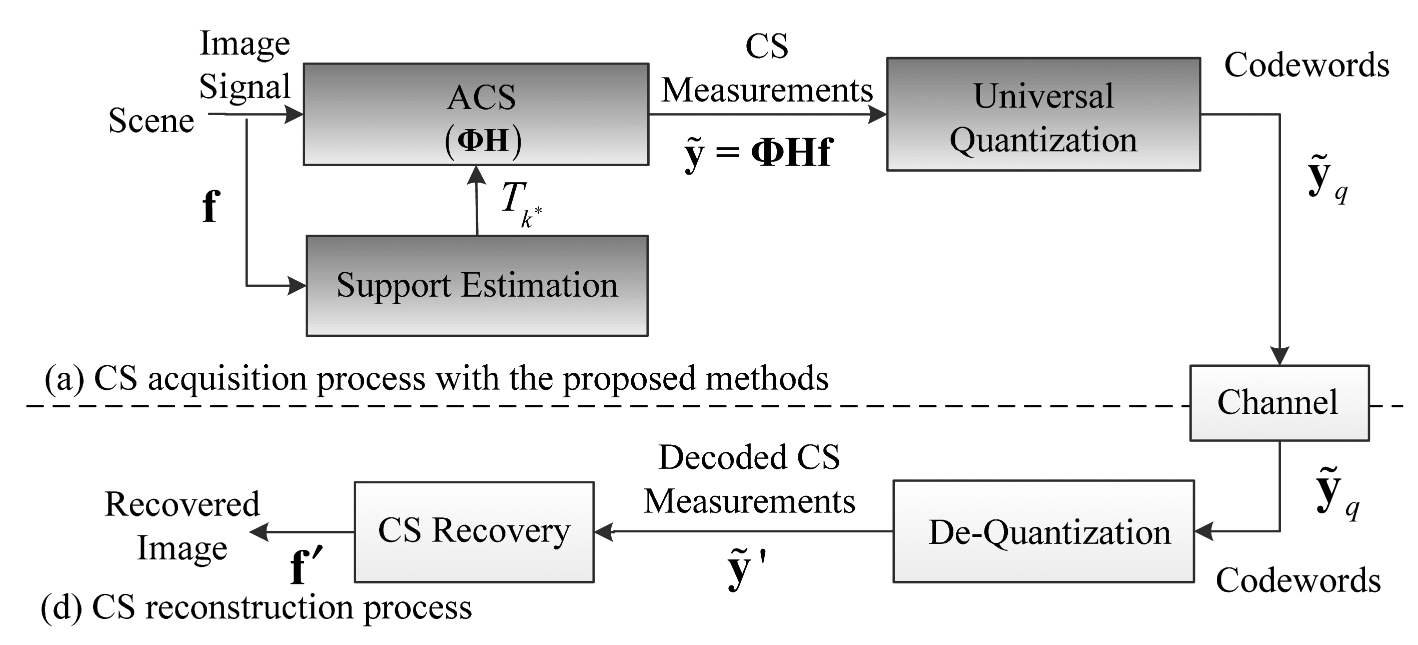
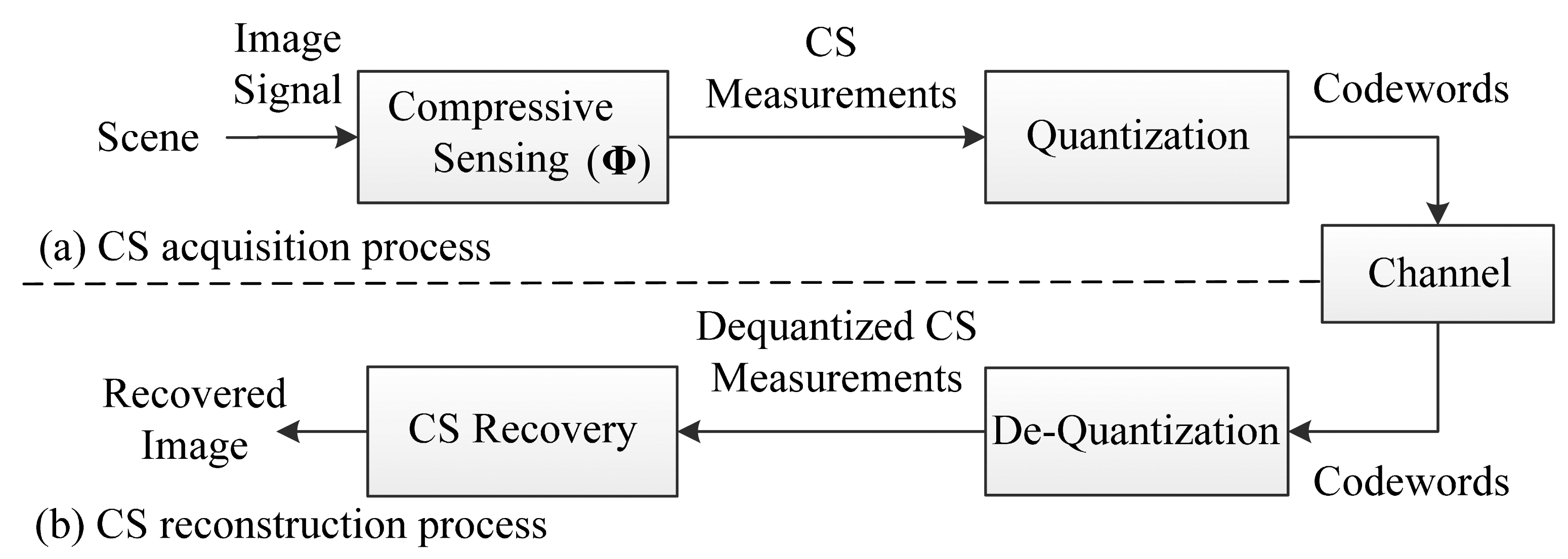
Compressive Sensing Imaging (CSI) is a new architecture for image acquisition and compression that has emerged in recent years, which enables acquiring and compressing a scene simultaneously [8–10]. Different from classical imaging solutions, CSI is able to acquire an image by measuring the scene a few times with a single-pixel camera [11] instead of sampling in high resolution with several million sensor elements, which breaks the traditional image acquisition architecture. With the lower sampling rate and fewer sensing elements in CSI [11], the imaging system is cheaper and less power is consumed. A typical CSI system mainly contains two processes, as shown in Figure 1. In the Compressive Sensing (CS) acquisition process, an input image is firstly measured via a measurement matrix Φ in a reduced dimensionality instead of full image resolution. Then the resulting CS measurements are quantized into a set of codewords, and these codewords are transmitted to the receiver via a channel. In CS reconstruction process, the received codewords are dequantized into CS measurements and the image is reconstructed by a CS recovery program.

Great effort has been put on the development of efficient CSI systems in recent years including the hardware application and algorithm design. A single-shot Complementary Metal-Oxide-Semiconductor (CMOS) image-sensor [12] performs CS at the Analog/Digital (A/D) conversion stage. Dadkhah et al. [13] reviewed different hardware implementations and important practical issues of CS encoding in CMOS sensor technologies. Chen et al. [14] solved the problem of wide-area video surveillance systems based on the parallel coded aperture CSI system. With all these CSI systems, the cost and complexity of image-sensor deployment could be well reduced and the low-complexity image/video acquisition can be designed by shifting the computational burden to the reconstruction process. An example is shown in [15] proving that CS provides great energy efficiency for sensing operations in Wireless Sensor Networks (WSNs).

In practical CSI applications, CS acquisition is assumed to be implemented in some analog image-acquisition hardware like a single-pixel camera [11]. The acquired CS measurements are real-valued, which has a large amount of data for storage and transmission. Therefore, the lossy compression of CS measurements is required in the CS acquisition process. The design of efficient lossy compression of CS acquisition will raise two questions: how to adaptively sparsify the image signal for better CS reconstruction, and how to efficiently quantize the real-valued CS measurements. We analyze these two questions in the following two paragraphs.

At the CS acquisition stage, it is known that a certain degree of sparsity of the original signal is important for CS reconstruction. If the original signal is not sparse enough, the reconstruction quality will degrade due to the noise folding effect. Arias-Castro et al. [16] studied this problem in a practical CS system. Laska et al. [17] showed that a compressible signal could only be recovered by part of its important coefficients, and the remaining coefficients will cause the noise folding effect, which seriously degrades the reconstruction quality. In order to reduce the noise folding effect, the simple Discrete Cosine Transform (DCT) coefficients truncation method [18] was applied in CS-based image/video coding to improve its Rate-Distortion (R-D) performance. However, it does not consider the variation of sampling rate which is the main factor for deciding how many important DCT coefficients can be accurately recovered for the reconstruction of the original signal. Mansour et al. proposed an adaptive compressive sensing method [19], which focuses on acquiring the large coefficients of a compressible signal to reduce the noise folding effect. However, this method simply used an empirical linear model to adapt the sampling rate.

At the CS measurements quantization stage, a general solution is to quantize the CS measurements with uniform scalar quantization considering the low-complexity requirements of the CSI system. However, it does not specifically consider the distribution characteristic of CS measurements. Goyal et al. [20] and Boufounos et al. [21] analyzed the quantization problem of CS measurements with a simple scalar quantization. The classical Probability Density Function (PDF)-based quantization [22] was adopted for this problem, which could exploit the distribution characteristic of the signal. Sun et al. [23] proposed an R-D optimized quantization for CS measurements based on the classical PDF-based quantization, which exploits the distribution characteristic of CS measurements. However, the direct implementation of PDF-based quantization will cause high computational complexity, since the PDF needs to be obtained in advance for CS measurements of each input image.

The main contribution of this paper is to develop an efficient lossy compression solution for CS acquisition of images in the CSI system, by considering both the image signal sparsification and CS measurements quantization. First, we propose an adaptive compressed sensing method to make the image signal sparser for CS acquisition, such that the reconstruction quality can be improved by reducing the noise folding effect. The proposed adaptive compressive sensing method truncates the image coefficients to retain some large coefficients according to the sampling rate. Second, we design a low-complexity universal quantization for the CS measurements by establishing a universal probability model without knowing any a priori information about the input image. Finally, the proposed adaptive compressive sensing and universal quantization methods are incorporated into the CSI system. Simulation results show that the proposed lossy compression solution for CS acquisition in the CSI improves its R-D performance and reduces its computational complexity compared with the conventional solution.

The rest of the paper is organized as follows: in Section 2, an adaptive compressive sensing method for CS image acquisition is presented. In Section 3, a universal quantization method is introduced for quantization of CS measurements. Then we provide the lossy compression solution of CS acquisition in the CSI system with the proposed adaptive compressive sensing and universal quantization methods in Section 4. Simulation results are shown in Section 5. Finally, we conclude the paper in Section 6.

2. Adaptive Compressive Sensing Method for CS Acquisition

In traditional signal acquisition systems, the analog signals are often low-pass filtered to limit their bandwidth before acquisition based on the Shannon-Nyquist sampling theorem [1]. The reconstruction quality could be improved by reducing the aliasing effect which is caused by the unlimited bandwidth of the signal. In a CS acquisition system, the reconstruction quality will degrade due to the noise folding effect caused by lack of sparsity of the signal. We will make the image sparser for CS acquisition in CSI system to improve the reconstruction quality. More specifically, we sparsify the image by retaining only a number of large coefficients according to the sampling rate.

2.1. Overview of Related Concepts in CS

The Compressive Sensing (also known as Compressive Sampling, CS) theory [24,25] enables to directly acquire the compressed signal with a few random projections and recover the signal from the projections. We suppose that f ∈ ℜ^N is a discrete signal, and denote its coefficients in the sparsifying basis Ψ ∈ ℜ^N×N by x ∈ ℜ^N Signal f is considered to be k-sparse with respect to Ψ if and only if k coefficients are non-zero. According to the CS theory, we can acquire the k-sparse signal f as follows:

$$\begin{array}{ccc}\mathbf{\text{y}}=\mathbf{\Phi }\mathbf{\text{f}}& \text{with}& y_i=\langle {\varphi }_i,\mathbf{\text{f}}\rangle ,i=1\dots n\end{array}$$

(1)

where y ∈ ℜⁿ (n ≪ N) is the CS measurements and Φ=[ϕ₁,ϕ₂,…,ϕ_n]^T ∈ ℜ^n×N is the measurement matrix that is incoherent with Ψ. The Sampling Rate (SR) is defined as:

$$SR=n/N$$

(2)

Supposing that Φ and Ψ satisfy the Restricted Isometry Property (RIP) condition of order k [24], then the coefficients x can be exactly recovered by solving the following optimization problem:

$$\begin{array}{cccc}\underset{\mathbf{\text{x}}\in {\Re }^N}{\text{min}}& {\parallel \mathbf{\text{x}}\parallel }_1& \text{s.t.}& \mathbf{\text{y}}=\mathbf{\Phi }\mathbf{\Psi }\mathbf{\text{x}}\end{array}$$

(3)

Finally the reconstructed signal is obtained as f̃ = Ψ^–1x̃ with the solution x̃ of Equation (3). In practical application, the coefficients x are not strictly sparse but compressible. In this case, the sorted coefficients of x in decreasing order often obey a power law [26]. Then x̃ contains the most significant coefficients of x, which provides a good approximation of the signal [24,27]. Moreover, CS measurements y will be corrupted by quantization noise [28]. Thus, the practical CS acquisition model in Equation (1) can be described more precisely as:

$$\mathbf{\text{y}}=\mathbf{\Phi }\mathbf{\text{f}}+\mathbf{\text{e}}$$

(4)

where e is the quantization noise bounded by a noise power ε.

Let T_k be the indices of the largest k values of x, and x_Tk be the k-sparse approximation of x. Candès et al. [26] and Donoho [25] stated that if Φ and Ψ satisfy certain RIP condition and the number of CS measurements is sufficient enough, that is:

$$n\ge O(klog(N/k))$$

(5)

then k largest values of x can be recovered stably from n CS measurements by solving the relaxed l₁ minimization problem [21]:

$$\begin{array}{cccc}\underset{\mathbf{\text{x}}\in {\Re }^N}{\text{min}}& {\parallel \mathbf{\text{x}}\parallel }_1& \text{s.t.}& {\parallel \mathbf{\Phi }\mathbf{\Psi }\mathbf{\text{x}}-\mathbf{\text{y}}\parallel }_2\le \varepsilon \end{array}$$

(6)

The solution x_* to Equation (6) obeys

$${\parallel {\mathbf{\text{x}}}^{*}-\mathbf{\text{x}}\parallel }_2\le C_0\varepsilon +\frac{C_1}{\sqrt{k}}{\parallel {\mathbf{\text{x}}}_{T_k^c}\parallel }_1$$

(7)

where C₀ and C₁ are constants.

Equation (7) shows that the reconstruction error of x depends on two error terms C₀ε and $\frac{C_1}{\sqrt{k}}{\parallel {\mathbf{\text{x}}}_{T_k^c}\parallel }_1$. The first term is proportional to the noise power and the second term is proportional to ${\parallel {\mathbf{\text{x}}}_{T_k^c}\parallel }_1$ (the l₁ norm of “tail” part of x), which will cause the noise folding effect [17]. The first error term will be considered in Section 3 to reduce the reconstruction error.

In this section, we consider the second term. Supposing the CS measurements ỹ = ΦΨx_Tk can be obtained from the k-sparse approximation x_Tk of x, we recover x with ỹ instead of y. The solution x^* to Equation (3) obeys ‖x^* – x_Tk‖₂ = 0 and:

$${\parallel {\mathbf{\text{x}}}^{*}-\mathbf{\text{x}}\parallel }_2={\parallel {\mathbf{\text{x}}}_{T_k^c}\parallel }_2$$

(8)

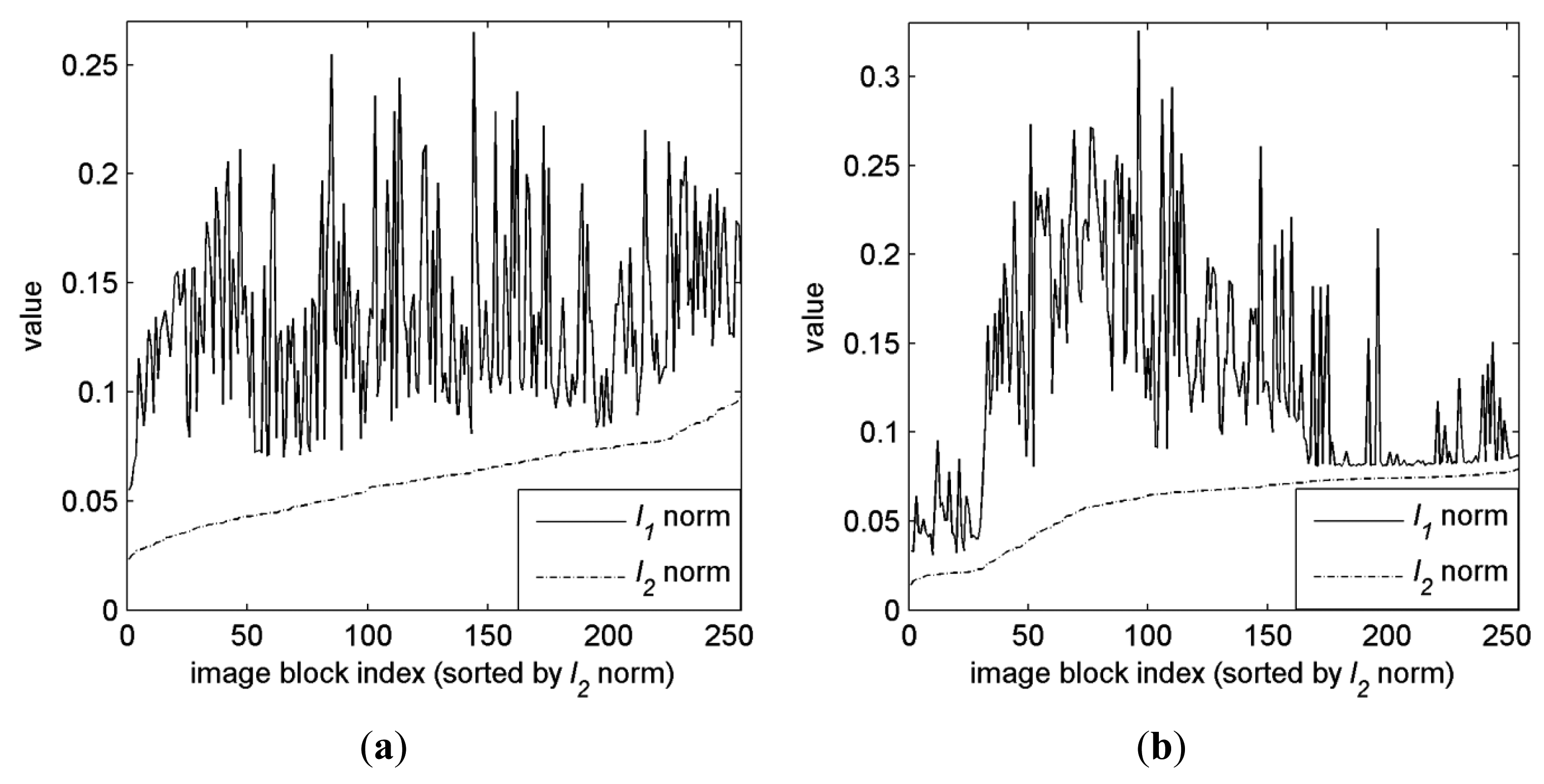
It is shown that solving Equation (3) with CS measurements ỹ results in an error in Equation (8). The error will be the second term in Equation (7) when y is used (without quantization). Generally, the l₁ norm in Equation (7) is often greater than the l₂ norm in Equation (8) for a “tail” part of the same compressible signal [19]. An example is shown in Figure 2, in which l₁ norm is often greater than l₂ norm for the DCT coefficients of 16 × 16 blocks in an image. So it is possible to achieve better CS reconstruction quality by recovering x with ỹ obtained from sparsified coefficients x_Tk In this section, we design an adaptive compressive sensing method which adaptively sparsifies the compressible signal for CS acquisition.

2.2. Adaptive Compressive Sensing Method

Generally, the conventional CS approach acquires all the values of the signal coefficients without sparsifying by truncating the small ones. If the signal is not sparse enough, it may result in poor reconstruction quality due to the noise folding effect, especially when the sampling rate is low. On the other hand, if we truncate too many values of the signal, the reconstruction quality may also degrade.

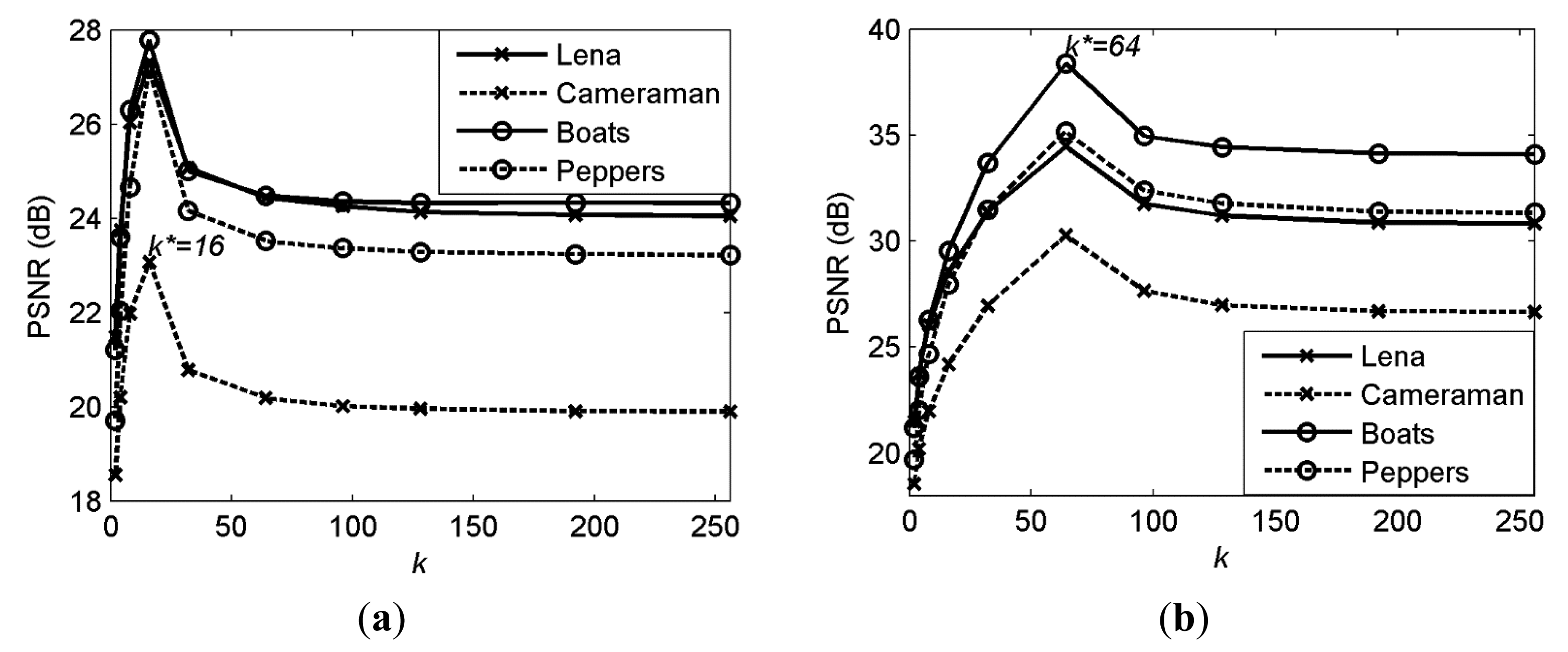
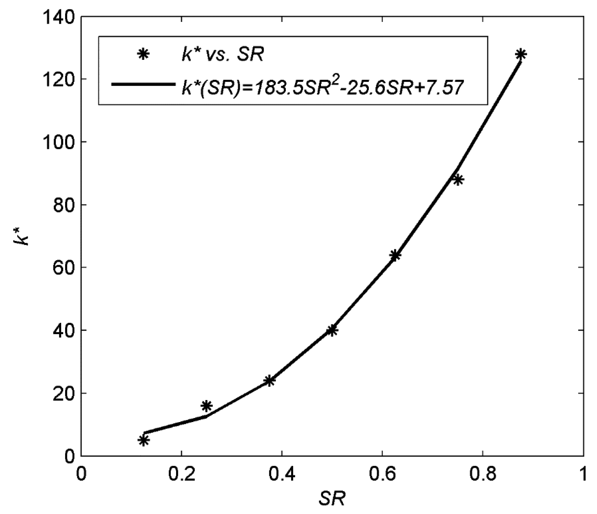
We truncate a part of small values of the signal coefficients according to the sampling rate. To achieve this, we aim to find the optimal truncation point k^* as follows:

$$k^{*}=\underset{k\in 1,2,\dots ,N}{\text{arg min}}{\parallel {\widetilde{\mathbf{\text{x}}}}_{T_k}-\mathbf{\text{x}}\parallel }_2$$

(9)

where x̃_Tk is the CS reconstruction of sparsified coefficients x_Tk via Equation (3) with CS measurements ỹ = ΦΨx_Tk ∈ ℜⁿ and Φ ∈ ℜ^n×N The Sampling Rate (SR) is defined in Equation (2). Equation (9) can be solved by searching all the truncation points, which has a high computational complexity. Therefore, rather than solving Equation (9), we try to establish a truncation point model to describe the relationship between k^* and SR for images to reduce its computational complexity. We examine the performance of the CS reconstruction at different truncation points for the DCT coefficients of the image blocks. Different sampling rates are tested for each image. For each sampling rate, the optimal truncation point k^* is obtained from Equation (9). Figure 3 shows the reconstruction Peak Signal-to-Noise Ratio (PSNR) (PSNR is obtained by firstly calculating the mean squared error (MSE) between the reconstructed signal and the original signal and then transformed to PSNR). For SR = 1/4, 5/8 on four test images, in which the optimal truncation point is k^* = 16 for SR = 1/4 and k^* = 64 for SR = 5/8. We can observe that the optimal truncation point for different images mainly depends on the sampling rate. Therefore, we first calculate k^* (averaging the values for all test images) at different sampling rates, and then fit their relationship with a quadratic polynomial function as shown in Figure 4, in which the model has been established as k^*(SR)=183.5·SR²–25.6·SR+7.57.

Once k^* is obtained, an optimal truncation indices T_k* can be determined. Then x could be truncated with T_k*. Here, we define a truncating matrix as:

$$\mathbf{\text{W}}=\text{Diag}(\mathbf{\text{w}})\in {\Re }^{N\times N}$$

(10)

where:

$$\begin{array}{cc}\mathbf{\text{w}}={[w_1,\dots ,w_i,\dots ,w_N]}^T,& w_i=\{\begin{array}{cc}\begin{array}{cc}1,& i\in T_{k^{*}}\\ 0,& i\in {T_{k^{*}}}^c\end{array},& i=1\dots N\end{array}\end{array}$$

(11)

Then the truncated coefficients can be calculated as:

$${\mathbf{\text{x}}}_{{\text{T}}_{k^{*}}}=\mathbf{\text{Wx}}$$

(12)

The x_Tk* in Equation (12) is the truncated coefficients from x. In the CS acquisition process, we can acquire x_Tk* instead of x to reduce the reconstructed error. At the reconstruction stage, we recover the coefficients from the CS measurements ỹ = ΦΨx_Tk*, which could be solved as follows:

$$\begin{array}{cccc}\underset{\mathbf{\text{x}}\in {\Re }^N}{\text{min}}& {\parallel \mathbf{\text{x}}\parallel }_1& \text{s.t.}& \mathbf{\Phi }\mathbf{\Psi }\mathbf{\text{x}}=\mathbf{ỹ}\end{array}$$

(13)

The solution of Equation (13) is the reconstructed coefficients from the CS measurements ỹ = ΦΨWx

3. Proposed Universal Quantization for CS Measurements

In practical CSI system, the real-valued CS measurements ỹ = [ỹ₁,…,ỹ_i,…, ỹ_n]^T obtained in Section 2 need to be further quantized to codewords ỹ_Q = [ỹ_1,Q,…,ỹ_i,Q,…, ỹ_n,Q]^T for processing and transmission, which can be described as:

$${ỹ}_{i,Q}=Q({ỹ}_i),i=1\dots n$$

(14)

where Q is the quantization function. The efficient CS measurements quantization is an important part of the lossy compression for CS acquisition, which reduces the reconstruction error in Equation (7) as mentioned in Section 2. In this section, we proposed a universal quantization method for the CS measurements of any input image. For simplicity, we use y_i and y instead of ỹ_i and ỹ_i in this section, respectively.

3.1. Universal Probability Modeling for CS Measurements

We first model the probability distribution of CS measurements, as it is related with the quantization design. Generally, we assume that the values of measurement matrix Φ=[ϕ₁,…,ϕ_i,…,ϕ_n]^T∈ ℜ ^n×N,i=1…n are a Gaussian distribution with zero mean and variance 1/n [26,29]. Then it is easy to know that y_i = ϕ_ix,i = 1…n is also a Gaussian distribution when the dimension N of the signal x ∈ ℜ^N is very large according to the Central Limit Theorem. That is y_i ∼ N(0,σ²) [17], where the variance σ² is related with CS measurements. Its Probability Density Function (PDF) is:

$$f_{\text{N}(0,{\sigma }^2)}(y)=\frac{1}{\sigma \sqrt{2\pi }}exp\left(-\frac{y^2}{2{\sigma }^2}\right)$$

(15)

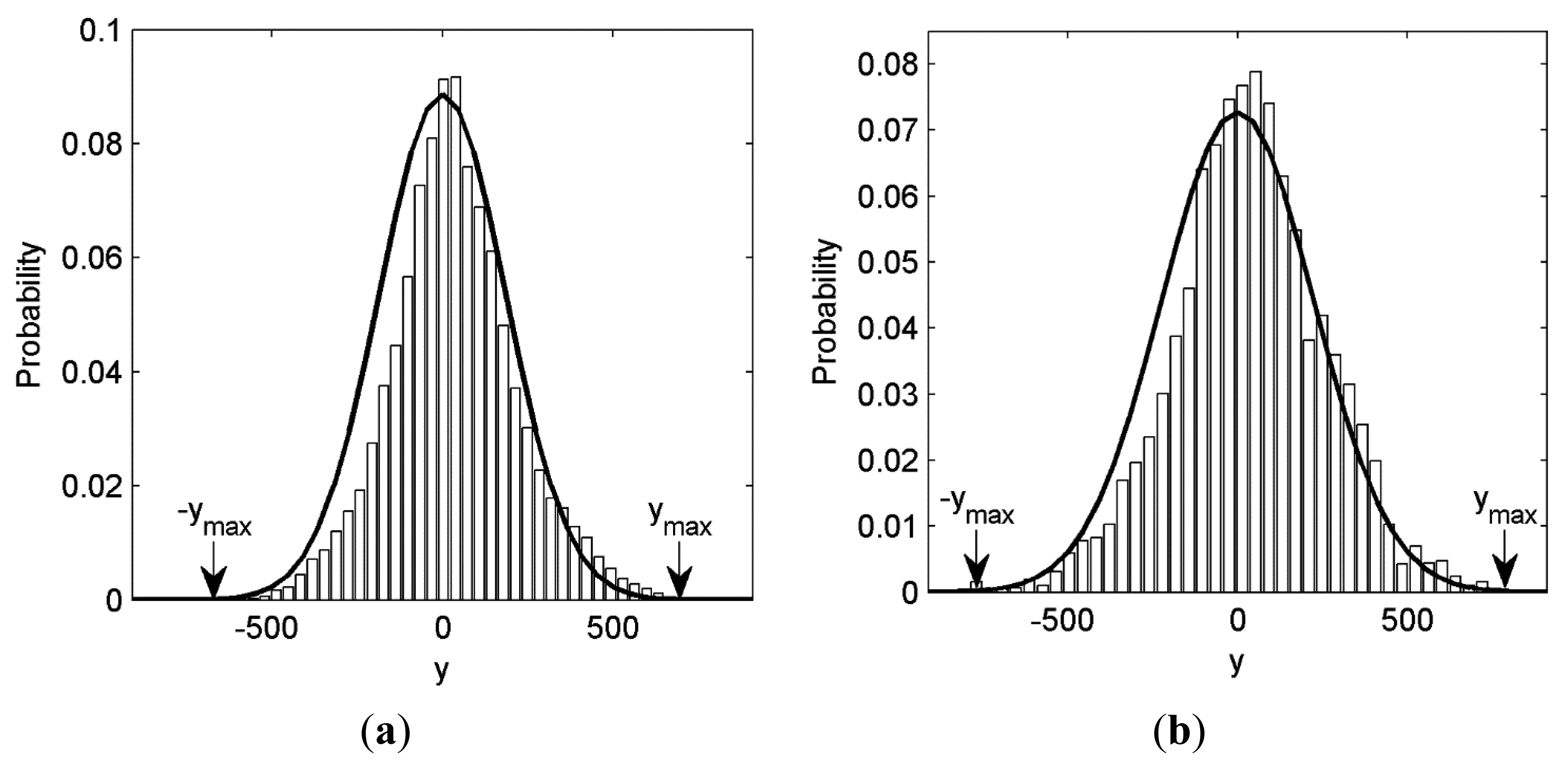
The histogram of CS measurements from test images Lena and Cameraman are depicted in Figure 5, together with the fitted curve of y_i ∼ N(0,σ²), where σ² is the variance of CS measurements. It is shown that the CS measurement obeys Gaussian distribution well. In practical CSI system, the CS measurements are within the range [–y_max, y_max], where y_max is the maximal value of all CS measurements. The probability fraction that outside the range is often very small as shown in Figure 5. Thus we only consider the range [–y_max, y_max] in Equation (15). Although the real y_max is unknown in the modeling procedure, it can be approximated by y_max ≈ d · σ instead, where d is an empirical parameter ranging from 3 to 5 [30]. We firstly divide the range [–d·σ,d·σ] into M_max = 2^R_max equal intervals, where R_max>10 is a predefined large quantization rate (bits per CS measurement) for high-resolution approximation. Since the size Δ = d·σ/2^R_max–1 of the interval is small, the approximation error is bounded by Δ/2 Thus the probability F_k that y will be contained in the k-th (k = 1,2,…,M_max) interval can be approximated as follows:

$$\begin{array}{ll}{F}_k\hfill & \approx f_{\text{N}(0,{\sigma }^2)}(y_{(k)})\cdot \Delta \hfill \\ \hfill & =\frac{d}{2^{R_{max}-1}}\cdot \frac{1}{\sqrt{2\pi }}exp\left(-\frac{{y_{(k)}}^2}{2{\sigma }^2}\right)\hfill \end{array}$$

(16)

where y_(k) ∼ N(0,σ²) is the center point of k-th interval.

Let y′_(k) = y_(k)/σ, then we know that y′_(k) ∼ N(0,1). Then Equation (16) can be rewritten as:

$$\begin{array}{cc}{F}_k=\frac{d}{2^{R_{max}-1}}\cdot f_{\text{N}(0,1)}(y{\text{'}}_{(k)}),& k=1,2\dots ,M_{max}\end{array}$$

(17)

where f_N(0,1)(y′_(k)) is the standard Gaussian distribution.

It is shown in Equation (17) that F_k has no relationship with the acquired CS measurements or image. It can be immediately calculated from the standard Gaussian distribution. Then the discrete probability model of the CS measurements can be obtained in advance without knowing any information about the input image. This benefits the low-complexity quantization design.

3.2. Universal Quantization Design

Based on the universal probability model F_k Equation (17) derived above, we then implement the traditional PDF-based quantization [22] to optimize the R-D performance. However, this optimization problem has a higher computational complexity than other simple solutions, such as uniform quantization, etc. We aim to design an efficient look-up table based on the PDF-based quantization, such that the practical quantization of CS measurement can be achieved by a simple mapping operation.

From quantization theory [22], the PDF-optimized quantization can be obtained by solving the following optimization problem:

$$\underset{Q}{min}\Vert y-Q(y)\Vert$$

(18)

The solution of Equation (18) is as follows [22]:

$$\lambda (y)=\frac{{f_{\mathbf{\text{y}}}}^{1/3}(y)}{\int {f_{\mathbf{\text{y}}}}^{1/3}(y\text{'})dy\text{'}}$$

(19)

where f_y(y) is the PDF of the source y, and λ(y) is the function to determine the number of the quantization levels. Integrating λ(y) gives the fraction of the quantization reproduction levels. We equally divide the range y∈[–d·σ,d·σ] into M_max = 2^R_max intervals Δ = d·σ/2^R_max–1. Denoting y_(k) to be the center point of k-th (k=1,2,…,M_max) interval, then the fraction λ_k of the quantization reproduction levels in the k-th interval can be approximated as follows:

$$\begin{array}{ll}{\lambda }_k\hfill & \approx \lambda (y_{(k)})\cdot \Delta \hfill \\ \hfill & =\frac{{\left[f_{\text{N}(0,{\sigma }^2)}(y_{(k)})\cdot \Delta \right]}^{1/3}}{{\sum }_{<M_{max}>}{\left[f_{\text{N}(0,{\sigma }^2)}(y_{(k)})\cdot \Delta \right]}^{1/3}}\hfill \end{array}$$

(20)

Substituting Equation (20) with Equation (17), we can derive:

$$\begin{array}{cc}{\lambda }_k\approx \frac{{F_k}^{1/3}}{{\sum }_{<M_{max}>}{F_k}^{1/3}},& k=1,2\dots ,M_{max}\end{array}$$

(21)

Then the cumulative fraction Γ_K of the quantization reproduction levels from the first interval to the k-th interval can be calculated as follows:

$$\begin{array}{cc}{\Gamma }_K={\sum }_{k=1}^{k=K}{\lambda }_k,& K=1,2\dots ,M_{max}\end{array}$$

(22)

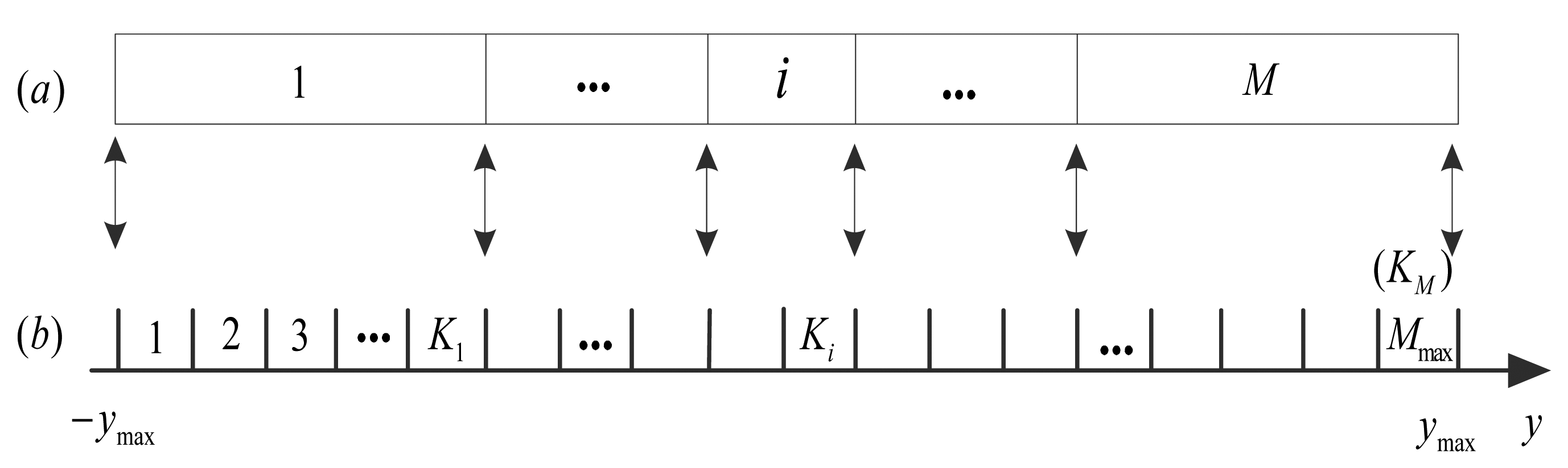
Since Γ_K is only related to universal probability model F_k which can be calculated by Equation (17) in advance, the designed quantization can be implemented efficiently as follows. For a given target quantization bits R (1<R≤R_max), the M = 2^R quantization cells can be mapped from the M_max = 2^R_max intervals via a mapping table, as shown in Figure 6. The interval index K_i in Figure 6b, which represents the rightmost interval for the i-th (1≤i≤M) quantization cell in Figure 6a is obtained as follows:

$$K_i=\underset{K\in 1,2,\dots ,M}{argmin}\left({\Gamma }_K-\frac{i}{M}\right)$$

(23)

Note that the interval index K_i (1≤i≤M) of R bits quantization is universal for the CS measurements of any input images. When quantizing a CS measurement y with the real value of y_max from specific image at the encoder, it is firstly quantized to an interval K_i in Figure 6b, and then it is mapped to the i-th quantization cell in Figure 6a. Then the output codeword i is transmitted to the decoder via a channel. At the decoder, the quantization reproduction value ŷ of the received quantization cell i can be reconstructed as follows:

$$\begin{array}{cc}{ŷ}_{(i)}=(K_{i-1}+K_i)\cdot \Delta /2-y_{max},& i=1,\dots ,M\end{array}$$

(24)

It is known that, the universal probability model F_k and λ_k in Equations (17) and (21) can be calculated in advance without knowing any information about the input image. Thus the cumulative fraction Γ_K can be calculated in advance. Then the designed quantization is only related with the maximum value of the CS measurements y_max and so is the de-quantization in Equation (24). Therefore, for quantizing the real-valued CS measurements from an input image, y_max is firstly obtained, then the quantization cell with given target bits R can be obtained easily via a linear mapping operation. The computational complexity of this quantization method is low, compared with classical PDF-optimized quantization, which has to first estimate the PDF and then calculate the quantization function in Equation (18) for each input image.

4. Lossy Compression Solution for CS Acquisition with the Proposed Methods

We incorporate the proposed Adaptive Compressive Sensing (ACS) and universal quantization methods into the CS acquisition process of CSI system to verify its lossy compression performance, as shown in Figure 7.

We design the ACS module for CS acquisition, which adaptively sparsifies the input image by truncating image coefficients in Figure 7a. In order to truncate the coefficients, ACS module requires optimal truncation indices T_k* to form a truncating parameter in Equation (10), so we design a support estimation module to estimate T_k* with truncation point model before acquisition in Figure 7a. After ACS module gets the estimated T_k* from support estimation module, the coefficients of the input image is then truncated and acquired. The resulting CS measurements are quantized by the proposed universal quantization module.

The procedure of this CSI system can be described as follows: denoting the image as f, the optimal truncation indices T_k* of f is first estimated by support estimation module. We build the truncating matrix W according to Equations (10) and (11) with T_k* and generate a matrix H = Ψ^TWΨ in ACS module to truncate the coefficients of the image. The CS measurements ỹ = ΦHf are quantized into codewords ỹ_q by universal quantization module. At the decoder, ỹ_q are de-quantized to ỹ′ by de-quantization module and finally f′ is reconstructed.

In practical application, we further consider the following two aspects to reduce the computational complexity. Firstly, we calculate the truncation point model in Equation (9) in advance for images which is stored and used by support estimation module. Secondly, the optimal truncation indices T_k* of the coefficients can be approximately obtained from the partially acquired CS measurements at the sampling rate SR = 0.1 with [31]. In this paper, we use the first k lowest frequency indices of DCT coefficients of the image in the zig-zag order.

5. Simulation Results and Analysis

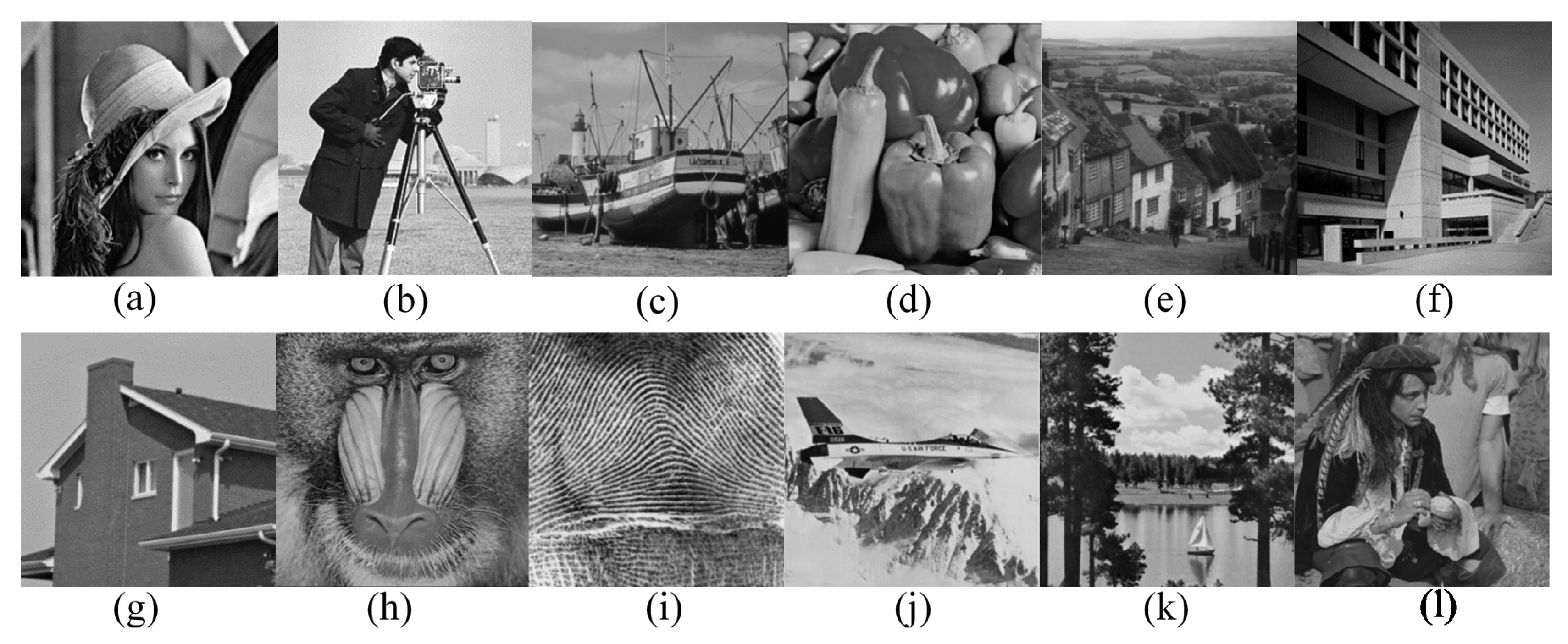
We verify the performance of the proposed solution for CS acquisition in CSI system in the following three aspects: (a) the proposed ACS method; (b) the proposed universal quantization method; (c) the R–D performance of the lossy compression for CS acquisition with proposed ACS and universal quantization methods. Twelve grayscale images of 256 × 256 resolution with different spatial characteristics are used for simulation as shown in Figure 8.

In the simulation, the images are first normalized to unit l₂ norm and then divided into 16 × 16 blocks. The values of the measurement matrix Φ are Gaussian distributed with zero mean and unit variance. We choose Discrete Cosine Transform (DCT) matrix as sparsifying basis Ψ. The CS scheme is performed over all blocks using the same measurement matrix Φ [32]. The standard l₁ minimization program [33] is used as the CS recovery algorithm. We measure the reconstruction performance in terms of a Peak Noise-to-Signal Ratio (PSNR) between the reconstructed and original images. All simulations were implemented using MATLAB R2011b and carried out on a computer with dual core CPU at 2.4 GHz and 2 GB RAM.

5.1. Performance of Proposed ACS Method

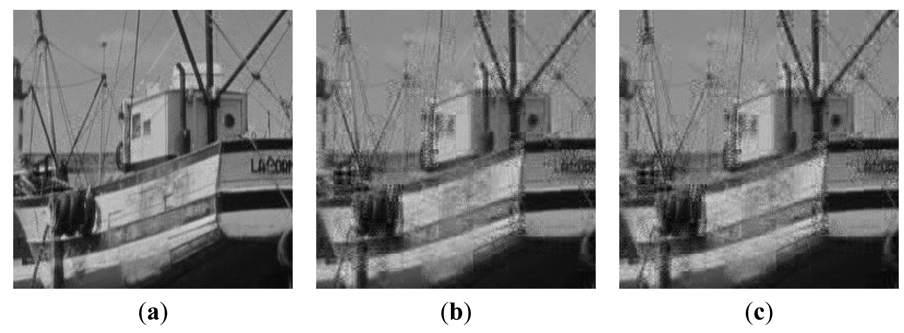
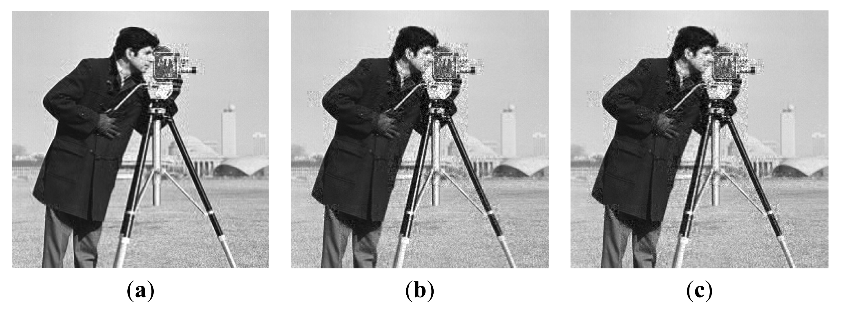
We compare the proposed ACS method (denoted “Proposed”) with two methods: (a) traditional CS method without adaptive technique (denoted “Baseline”); (b) the solution in [19] (denoted “Method [19]”). The simulation results are shown in

Table 1. PSNR (dB) comparison between the proposed method, baseline and Method [19].

Sampling Rate	Methods	Lena	Cameraman	Boats	Peppers	Average
SR = 1/4	Baseline	24.05	19.90	24.32	23.22	22.87
	Method [19]	24.49	20.33	24.63	23.71	23.29
	Proposed	27.64	23.17	28.29	26.91	26.50
SR = 5/8	Baseline	30.84	26.66	34.10	31.33	30.73
	Method [19]	31.34	27.14	24.54	31.91	31.23
	Proposed	34.50	30.29	38.42	35.18	34.60

. Our method achieves an average of 3.21∼3.63 dB PSNR gain comparing to other solutions at SR = 1/4, and 3.37∼3.87 dB PSNR gain at SR = 5/8.

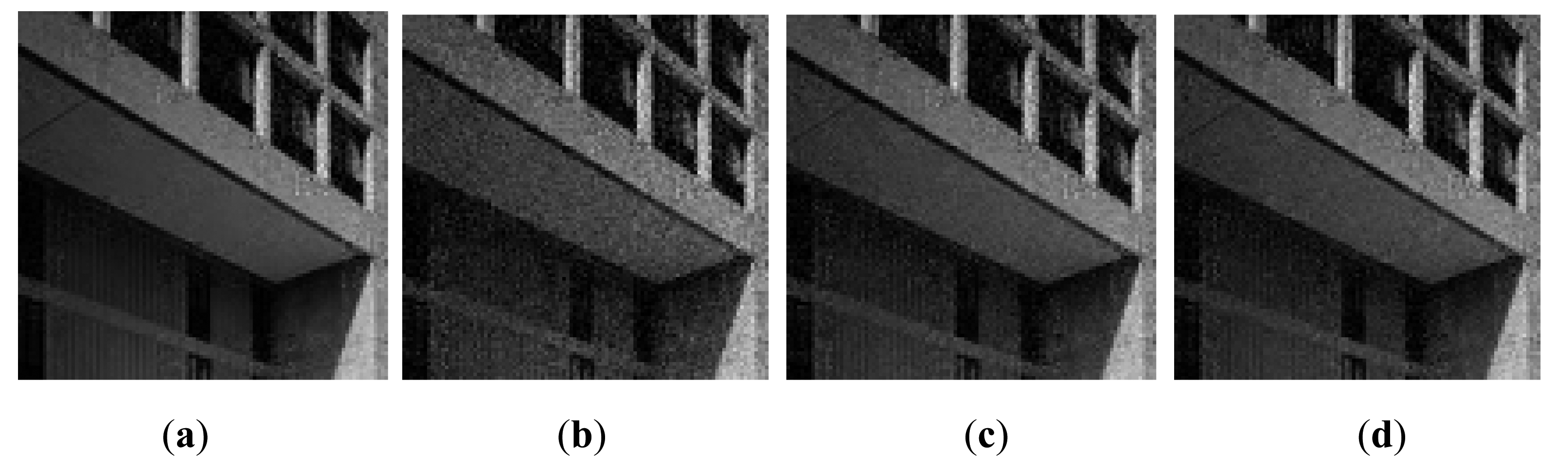
Figures 9 and 10 show the subjective quality of the reconstructed images for Boats and Cameraman at SR = 1/4 and SR = 5/8. We can see that our method provides superior visual quality of recovered images compared to other solutions.

5.2. Performance of Proposed Universal Quantization Method

The proposed universal quantization is compared to the uniform quantization and classical PDF-based quantization at fixed rate (without entropy coding). We empirically set d = 4.5 in Equation (17) for simulation. The quantization bits R is ranging from 2 to 8. The results are shown in

Table 2. The PSNR (dB) gains over “uniform quantization” at SR = 0.7.

Images	R = 3		R = 5
	PDF-Based Quantization	Universal Quantization	PDF-Based Quantization	Universal Quantization
Lena	4.06	3.95	1.98	1.79
Cameraman	3.87	3.97	1.57	1.56
Boats	4.51	4.23	2.68	2.25
Pepper	4.20	4.18	3.02	2.93
Goldhill	5.58	4.89	3.62	3.22
Bank	4.91	4.00	2.59	1.57
House	5.32	4.63	3.36	3.56
Baboon	5.28	4.48	1.84	1.87
Fingerprint	4.74	4.06	2.22	2.07
Jetplane	6.63	5.07	3.63	3.55
Lake	3.22	4.08	1.77	1.61
Pirate	6.31	5.24	4.46	3.42
Average	4.89	4.40	2.70	2.45

and Figure 11. Figures 12 and 13 show the subjective comparisons of these three methods. It is shown that the performance of our method is comparable with that of PDF-based quantization. Note that, the probability model in our method is established in advance without knowing any information about input image, while the probability model in PDF-based quantization needs to be calculated for each input image.

We further verify the computational complexity of the proposed universal quantization. Our method only requires a simple look-up table operation for CS measurements compression. In contrast, PDF-based quantization has to estimate the PDF for the CS measurements of each input image first and then calculate the quantization. Both of these two procedures have high computational complexity. The simulation times (with MATLAB) and theoretical complexity of universal quantization, uniform quantization, and PDF-based quantization are listed in

Table 3. Complexity comparison of three methods (R = 5, SR = 0.5).

Methods	Theoretical Complexity	Simulation Time (ms)
		Baboon 128 × 128	Bank 256 × 256	Cameraman 512 × 512
PDF-based Quantization	O(n)	1314	4517	20174
Uniform Quantization	O(1)	0.02	0.02	0.02
Universal Quantization	O(1)	2.84	2.89	2.88

. It is shown that the simulation time of the universal quantization is much lower than that of PDF-based quantization. Moreover, the computational complexity of the PDF-based quantization increases rapidly with the increase of the image resolution. By comparison, the computational complexity of the proposed universal quantization has no relation with the resolution of the input image. Comparing with uniform quantization, the simulation time of the universal quantization is a little high due to the look-up table operation; however, the R-D performance of the universal quantization is much better.

5.3. R-D performance of the Lossy Compression Solution of CS Acquisition

We evaluate the R-D performance of the proposed lossy compression solution of CS acquisition in CSI, which incorporates both the proposed ACS and universal quantization methods. We first examine the performance of the proposed CSI system in Figure 7 (denoted “Proposed”) and compare it with that of the traditional CSI system in Figure 1 (denoted “Baseline”), which uses the uniform quantization. The CS measurements are directly quantized without entropy coding. The sampling rate is SR =1/4, 3/8 and quantization bits R = 4, 5.

Table 4. PSNR (dB) comparison of the proposed solution and baseline solution.

Images	SR = 3/8, R = 5			SR = 1/4, R = 4
	Baseline	Proposed	Gain	Baseline	Proposed	Gain
Lena	24.1	25.6	+1.5	20.4	21.7	+1.3
Cameraman	21.2	22.6	+1.3	18.1	18.7	+0.6
Boats	24.6	26.0	+1.4	20.8	21.6	+0.8
Peppers	23.8	25.3	+1.5	19.7	20.9	+1.2
Goldhill	25.1	26.5	+1.4	21.1	22.4	+1.3
Bank	21.9	23.7	+1.8	18.4	20.0	+1.6
House	26.3	27.6	+1.3	21.6	22.9	+1.3
Baboon	24.0	24.9	+0.9	21.3	21.7	+0.4
Fingerprint	20.9	22.3	+1.4	17.8	18.8	+1.0
Lake	22.9	24.4	+1.5	19.1	20.2	+1.1
Pirate	24.6	26.1	+1.5	20.6	22.0	+1.4
Average	23.6	25.0	+1.4	20.0	21.0	+1.0

shows the results for eleven images. It is shown that the proposed solution increases the PSNR by 1.4 dB on average comparing to Baseline for SR = 3/8 and R = 5, and 1.0 dB for SR = 1/4 and R = 4. Moreover, we found that the PSNR gain for Bank is higher than that for Baboon, possibly because there are more texture details in Baboon (corresponding to more high frequency components), which is truncated by the ACS method.

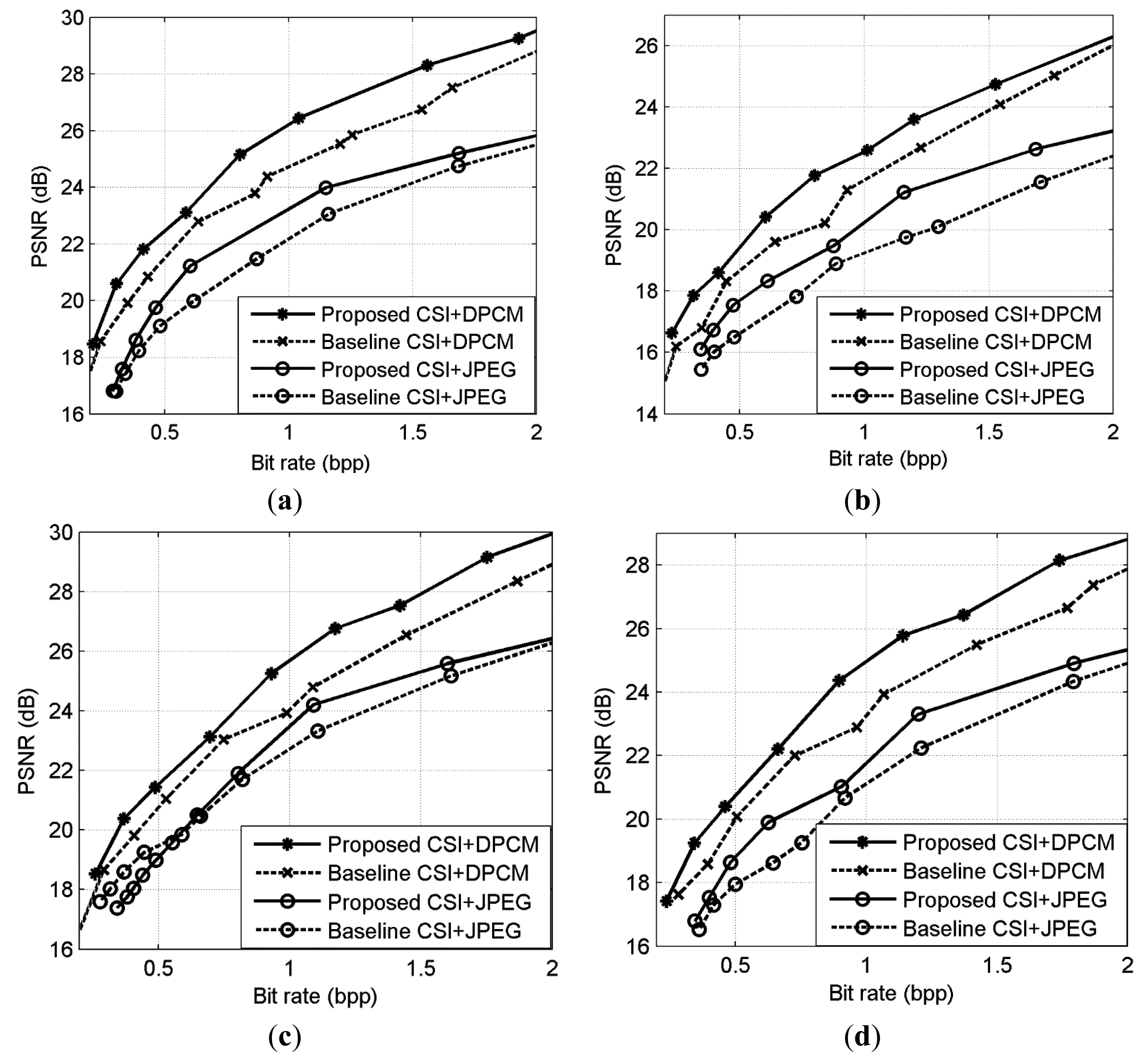
We then verify the performance of the proposed solution in practical compression application by incorporating Differential Pulse Code Modulation (DPCM) [34,35] into the proposed and baseline CSI systems for compression (denoted by “Proposed CSI + DPCM” and “Baseline CSI + DPCM” respectively). In “Proposed CSI + DPCM”, the real-valued CS measurements are compressed by DPCM encoder, and the reconstructed image is obtained by CS recovery.

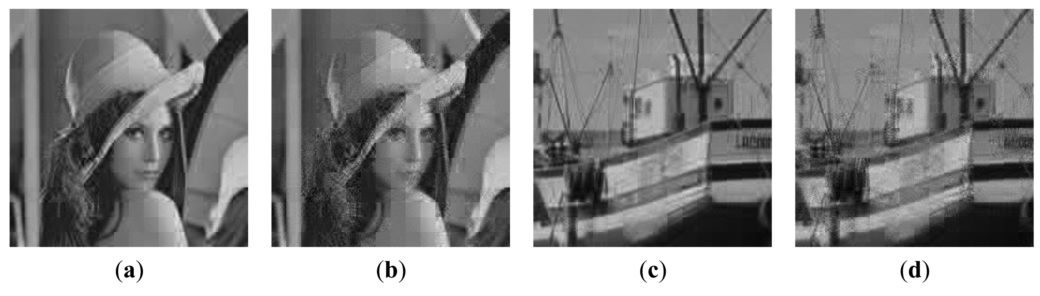
The R-D curve is the combination of all the best R-D points for each bit rate by searching all the sampling rates SR = {1/8,2/8,3/8,4/8,5/8,6/8,7/8} and quantization bits R = {1,2,3,4,5,6,7,8,9} [36]. Figure 14 shows the results for 4 images. We can see that the “Proposed CSI + DPCM” achieves up to 2dB PSNR gain comparing to “Baseline CSI + DPCM” solution. We further verify the performance of the proposed solution by incorporating JPEG [37,38] into the proposed and baseline CSI systems for compression (denoted by “Proposed CSI + JPEG” and “Baseline CSI + JPEG” respectively). The range of real-valued CS measurements is first mapped into 8-bit range 0–255, and then the CS measurements are sent to JPEG. The result is shown in Figure 14. It is shown that the “Proposed CSI + JPEG” achieves up to 2dB PSNR gain comparing to the “Baseline CSI + JPEG”. We also found that the“Proposed CSI + DPCM” outperforms “Proposed CSI + JPEG”. It is possibly because JPEG is designed for natural image compression, whose distribution characteristic is different from that of the CS measurements. The subjective results are shown in Figures 15 and 16, in which the proposed solution achieves better visual quality than that of the baseline solution.

6. Conclusions

In this paper, we have developed an ACS method and a universal quantization method for efficient lossy compression of CS acquisition in CSI systems. Simulation results show that the proposed solution achieves improved R-D performance and subjective quality of the CSI system; meanwhile, it has a low computational complexity.

References

- Unser, M. Sampling-50 years after Shannon. Proc. IEEE 2000, 88, 569–587. [Google Scholar]
- Li, C.; Jiang, H.; Wilford, P.; Zhang, Y.; Scheutzow, M. A new compressive video sensing framework for mobile broadcast. IEEE Trans. Broadcast. 2013, 59, 197–205. [Google Scholar]
- Akyildiz, I.F.; Melodia, T.; Chowdhury, K.R. A survey on wireless multimedia sensor networks. Comput. Netw. 2007, 51, 921–960. [Google Scholar]
- Pudlewski, S.; Melodia, T.; Prasanna, A. Compressed-sensing enabled video streaming for wireless multimedia sensor networks. IEEE Trans. Mob. Comput. 2012, 11, 1060–1072. [Google Scholar]
- Blanes, I.; Magli, E.; Serra-Sagrista, J. A tutorial on image compression for optical space imaging systems. IEEE Trans. Geosci. Remote Sens. Mag. 2014, 2, 8–26. [Google Scholar]
- Klein, M.E.; Aalderink, B.J.; Padoan, R.; de Bruin, G.; Steemers, T.A. Quantitative Hyperspectral Reflectance Imaging. Sensors 2008, 8, 5576–5618. [Google Scholar]
- Willett, R.; Duarte, M.; Davenport, M.; Baraniuk, R. Sparsity and structure in hyperspectral imaging. IEEE Signal Process. Mag. 2014, 31, 116–126. [Google Scholar]
- Wakin, M.; Laska, J.; Duarte, M.; Baron, D.; Sarvotham, S.; Takhar, D.; Kelly, K.; Baraniuk, R. An architecture for compressive imaging. Proceedings of the IEEE International Conference on Image Processing, Atlanta, GA, USA, 8–11 October 2006; pp. 1273–1276.
- Romberg, J. Imaging via compressive sampling. IEEE Signal Process. Mag. 2008, 25, 14–20. [Google Scholar]
- Takhar, D.; Laska, J.N.; Wakin, M.B.; Duarte, M.F.; Baron, D.; Sarvotham, S.; Kelly, K.F.; Baraniuk, R.G. A new compressive imaging camera architecture using optical-domain compression. Proc. IS&T/SPIE Symp. Electron. Imag. 2006, 6065. [Google Scholar] [CrossRef]
- Duarte, M.; Davenport, M.; Takhar, D.; Laska, J.; Sun, T.; Kelly, K.; Baraniuk, R. Single-pixel Imaging via Compressive Sampling. IEEE Signal Process. Mag. 2008, 25, 83–91. [Google Scholar]
- Oike, Y.; Gamal, A. CMOS image sensor with per-column ΔΣ ADC and programmable compressed sensing. IEEE J. Solid-St. Circ. 2013, 48, 318–328. [Google Scholar]
- Dadkhah, M.; Deen, M.; Shirani, S. Compressive sensing image sensors-hardware implementation. Sensors 2013, 13, 4961–4978. [Google Scholar]
- Chen, J.; Wang, Y.; Wu, H. A coded aperture compressive imaging array and its visual detection and tracking algorithms for surveillance systems. Sensors 2012, 12, 14397–14415. [Google Scholar]
- Razzaque, M.; Dobson, S. Energy-efficient sensing in wireless sensor networks using compressed sensing. Sensors 2014, 14, 2822–2859. [Google Scholar]
- Arias-Castro, E.; Eldar, Y. Noise folding in compressed sensing. IEEE Signal Process. Lett. 2011, 18, 478–481. [Google Scholar]
- Laska, J.; Baraniuk, R. Regime change: Bit-depth versus measurement-rate in compressive sensing. IEEE Trans. Signal Process. 2012, 60, 3496–3505. [Google Scholar]
- Zhang, Y.; Mei, S.; Chen, Q.; Chen, Z. A novel image/video coding method based on Compressed Sensing theory. Proceedings of the IEEE International Conference on Acoustics, Speech and Signal Processing, Las Vegas, NV, USA, 30 March–4 April 2008; pp. 1361–1364.
- Mansour, H.; Yilmaz, O. Adaptive compressed sensing for video acquisition. Proceedings of the IEEE International Conference on Acoustics, Speech and Signal Processing, Kyoto, Japan, 25–30 March 2012; pp. 3465–3468.
- Goyal, V.; Fletcher, A.; Rangan, S. Compressive sampling and lossy compression. IEEE Signal Process. Mag. 2008, 25, 48–56. [Google Scholar]
- Boufounos, P.T.; Baraniuk, R.G. Quantization of Sparse Representations. Proceedings of the Data Compression Conference, 2007. DCC ′07, Snowbird, UT, USA, 27–29 March 2007; pp. 378–387.
- Gray, R.; Neuhoff, D. Quantization. IEEE Tran. Int. Theory 1998, 44, 2325–2383. [Google Scholar]
- Sun, J.; Goyal, V. Optimal Quantization of Random Measurements in Compressed Sensing. Proceedings of the IEEE International Symposium on Information Theory, Seoul, Korea, 28 June–3 July 2009; pp. 6–10.
- Candès, E.J.; Romberg, J.; Tao, T. Robust uncertainty principles: Exact signal reconstruction from highly incomplete frequency information. IEEE Tran. Int. Theory 2006, 52, 489–509. [Google Scholar]
- Donoho, D.L. Compressed sensing. IEEE Tran. Int. Theory 2006, 52, 1289–1306. [Google Scholar]
- Candès, E.J.; Romberg, J.; Tao, T. Stable signal recovery from incomplete and inaccurate measurements. Comm. Pure Appl. Math. 2006, 59, 1207–1223. [Google Scholar]
- Cohen, A.; Dahmen, W.; DeVore, R. Compressed sensing and best k-term approximation. J. Am. Math. Soc. 2009, 22, 211–231. [Google Scholar]
- Candès, E.; Tao, T. Decoding by linear programming. IEEE Trans. Inf. Theory 2005, 51, 4203–4215. [Google Scholar]
- Li, X.; Lan, X.; Yang, M.; Xue, J.; Zheng, N. Universal and low-complexity quantization design for compressive sensing image coding. Proceedings of the IEEE International Conference on Visual Communications and Image Processing, Kuching, Malaysia, 17–20 November 2013; pp. 1–5.
- Rees, D. Essential Statistics, 4th ed.; Chapman & Hall/CRC: London, UK, 2001. [Google Scholar]
- Liu, H.; Song, B.; Qin, H.; Qiu, Z. An adaptive-ADMM algorithm with support and signal value dectection for compressed sensing. IEEE Signal Process. Lett. 2013, 20, 315–318. [Google Scholar]
- Gan, L. Block compressed sensing of natural images. Proceedings of the International Conference on Digital Signal Processing, Cardiff, UK, 1–4 July 2007; pp. 403–406.
- Candès, E.J.; Romberg, J. L1-Magic: Recovery of sparse signals via convex programming. Available online: http://www.acm.caltech.edu/l1magic/downloads/l1magic.pdf (accessed on 1 October 2014).
- Mun, S.; Fowler, J. DPCM for quantized block-based compressive sensing of images. Proceedings of the European Signal Processing Conference, Bucharest, Romania, 27–31 August 2012; pp. 1424–1428.
- Dinh, K.; Shim, H.; Jeon, B. Measurement coding for compressive imaging using a structural measurement matrix. Proceedings of the IEEE International Conference on Image Processing, Melbourne, Australia, 15–18 September 2013; pp. 10–13.
- Liu, H.; Song, B.; Tian, Fang; Qin, H. Joint sampling rate and bit-depth optimization in compressive video sampling. IEEE Trans. Multimed. 2014, 16, 1549–1562. [Google Scholar]
- Wallace, G. The JPEG Still Picture Compression Standard. J Commun. ACM 1991, 34, 30–44. [Google Scholar]
- MATLAB Central File Exchange. http://www.mathworks.com/matlabcentral/fileexchange/10476-jpeg-codec (accessed on 2 October 2014).