Markov Jump Linear Systems-Based Position Estimation for Lower Limb Exoskeletons

Abstract
: In this paper, we deal with Markov Jump Linear Systems-based filtering applied to robotic rehabilitation. The angular positions of an impedance-controlled exoskeleton, designed to help stroke and spinal cord injured patients during walking rehabilitation, are estimated. Standard position estimate approaches adopt Kalman filters (KF) to improve the performance of inertial measurement units (IMUs) based on individual link configurations. Consequently, for a multi-body system, like a lower limb exoskeleton, the inertial measurements of one link (e.g., the shank) are not taken into account in other link position estimation (e.g., the foot). In this paper, we propose a collective modeling of all inertial sensors attached to the exoskeleton, combining them in a Markovian estimation model in order to get the best information from each sensor. In order to demonstrate the effectiveness of our approach, simulation results regarding a set of human footsteps, with four IMUs and three encoders attached to the lower limb exoskeleton, are presented. A comparative study between the Markovian estimation system and the standard one is performed considering a wide range of parametric uncertainties.1. Introduction
Research and development on robotic devices for rehabilitation and assistance have received much attention in the last few years. Alternative designs of exoskeletons for upper and lower limbs have been proposed in the literature (e.g., [1–3]). We can cite force and impedance controls as examples to suit the patient's gait pattern and to provide new approaches for enhancing balance and muscle strengthening.
As the control approaches for this class of robots are generally performed based on absolute and relative angles of their segments, they depend on reliable and accurate position measurements. In this sense, inertial measurement units (IMUs) have been successfully applied to gait identification (e.g., [4,5]) and in control approaches to provide stability and gait-pattern adaptation during walking. In [6], for instance, the use of an IMU is proposed to estimate the knee joint angle of a lower limb orthosis. The resulting measurement provides redundant information to the control system, conceived to dynamically adapt the impedances of the orthosis joints.
In [7], switch sensors based on force sensitive resistors (FSR) and IMUs are used to determine the phases of the human gait, namely heel-strike, toe-off, stance and swing phases. The authors use gait-phase identification to improve the accelerometer performance. However, it does not provide a good indication of accelerometer reliability of all lower limb segments. Since the dynamics are different for each segment during walking, this approach provides a good result only for the foot segment. The acceleration measurements deteriorate when we take into account other members of lower limbs.
In order to deal with the performance limitations of lower limb exoskeletons, in [8], three accelerometers are used instead of identifying gait phases, in an approach based on Kalman filter and genetic algorithm optimization. A robust estimation version of this approach is proposed in [9], whose effectiveness is verified in extreme conditions of parametric uncertainties.
It is known that when the dynamic acceleration increases, the number of reliable accelerometers reduces at a certain instant of time. Consequently, in some segments, like the trunk and foot, the high incidence of dynamic accelerations can degrade the angular estimation. Furthermore, human walking has great variability and unpredictability related with the speed and length of each step, which cause different patterns of dynamic accelerations in each segment. In order to deal with this problem, we propose a model that encompasses the influence of whole dynamic accelerations in a lower limb exoskeleton.
This model is developed based on Markovian systems, which are a particular class of randomly time varying-systems. The main feature of this approach is that the probability of the system being in a different configuration in the next time instant depends only on the present system configuration, regardless of the time instant considered. Markovian modeling has been used to solve control problems in robotic systems. For example, in [10], a position Markovian
 ∞ controller was implemented in an underactuated manipulator, subject to abrupt changes on its configuration. It is conceived of to deal with a set of joint faults.
In this paper, we propose a new approach based on the Markovian model to estimate angular positions in lower limbs exoskeleton to overcome the accelerometer reliability problem over all gait phases. In contrast to [4–9], where the position estimations are based on an individual link configuration, the proposed method takes into account a collective modeling of all inertial sensors attached to the exoskeleton.
In order to show the effectiveness of the estimation model proposed, we present simulations based on a set of human footsteps, with four IMUs and three encoders attached to the lower limb exoskeleton. A comparative study between estimations based on Markovian and standard Kalman filters is performed, considering a wide range of parametric uncertainties.
This paper is organized as follows: Section 2 presents the accelerometer and gyroscope models, the standard sensor fusion strategy and the proposed Markov Jump Linear Systems (MJLS)-based model. Section 3 presents the Markovian Kalman filter algorithm and the required conditions to select the best information from each sensor. Finally, Section 4 presents simulated results and discussions.
2. Markovian Estimation Model
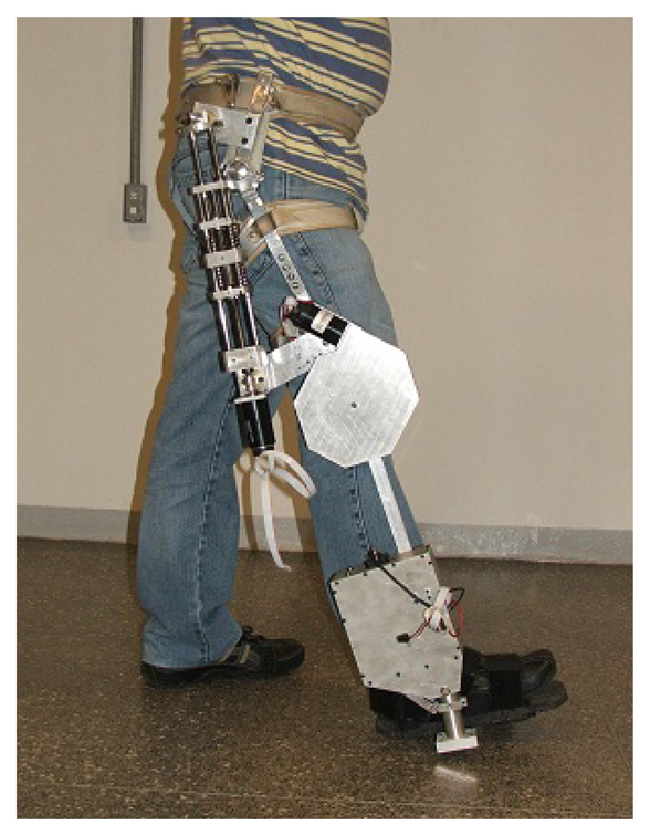
In this section, the Markovian model and the sensor fusion strategy designed to estimate the absolute and relative angular positions of exoskeletons for lower limbs are presented. The proposed approach will be applied to the exoskeleton, Exo-Kanguera, where rehabilitation protocols have been used to help stroke and spinal cord injured patients during walking rehabilitation. It is driven by a series of elastic actuators that allow the implementation of impedance control, ensuring patient safety and the ability to define different interaction behaviors. Figure 1 shows a user with the Exo-Kanguera.
In the following, gyroscope and accelerometer models are described. Standard sensor fusion approaches for an individual IMU and the proposed MJLS-based model, which includes signals of all IMUs attached to the exoskeleton, are presented.
2.1. Gyroscope and Accelerometer Models
The IMUs are attached to each segment of the body, as shown in Figure 2. Regarding the gyroscope measurement, the angular velocity of the link where the IMU is attached, θ̇(t), at a given instant, t, is modeled as:
Analogously, the acceleration of the link, a(t), at a given instant, t, is modeled as:
Since the variances, , , and , are known, simulated signals for θ̇g and aa can be generated considering a set of curves for θ̇ and a, defined from normal gait patterns.
2.2. Sensor Fusion Strategy
Standard sensor fusions based on Kalman filters take into account the gyroscope signal as the main source for position estimation. They use the accelerometer signal as a redundant information to correct the estimated value from the gyroscope, usually corrupted by integration errors. The estimated angular velocity and bias from the gyroscope are given by:
Taking the difference between real and estimated values, we obtain:
Hence, the state space representation of the estimation system is obtained as:
The angular position obtained from the accelerometer is given by:
The output equation of the state space representation is given by the difference between the estimated position from the accelerometer and estimated position from the gyroscope, that is,
Therefore,
The final estimated values for the angular position and gyroscope bias are given by:
2.3. Markovian Estimation Model
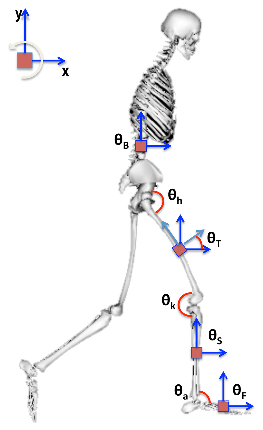
In this section, we propose a new MJLS model for angular position estimation of lower limb exoskeletons. Considering one leg of the exoskeleton, Exo-Kanguera (see Figures 1 and 2), the following absolute and relative angles are defined:
Absolute angles: θB (body/trunk), θT (thigh), θS (shank), θF (foot);
Relative angles: θh (hip), θk (knee), θa (ankle).
The spatial configuration of the exoskeleton, Exo-Kanguera, at a given instant of time, can be obtained by estimating one absolute angle and three relative angles. The absolute angle is obtained by the sensor fusion approach presented in Section 2.2. The relative angles are measured by encoders coupled to the joints of the exoskeleton.
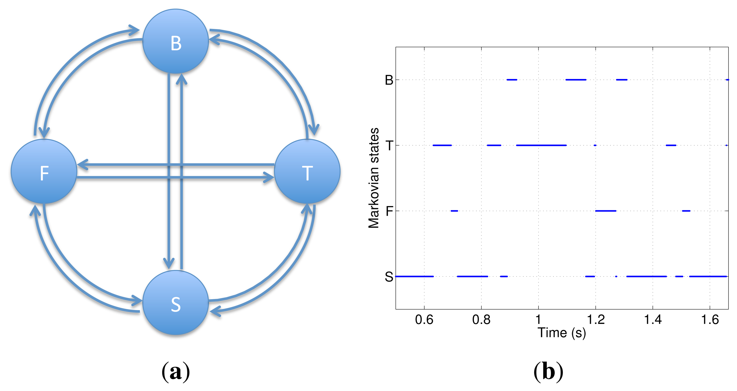
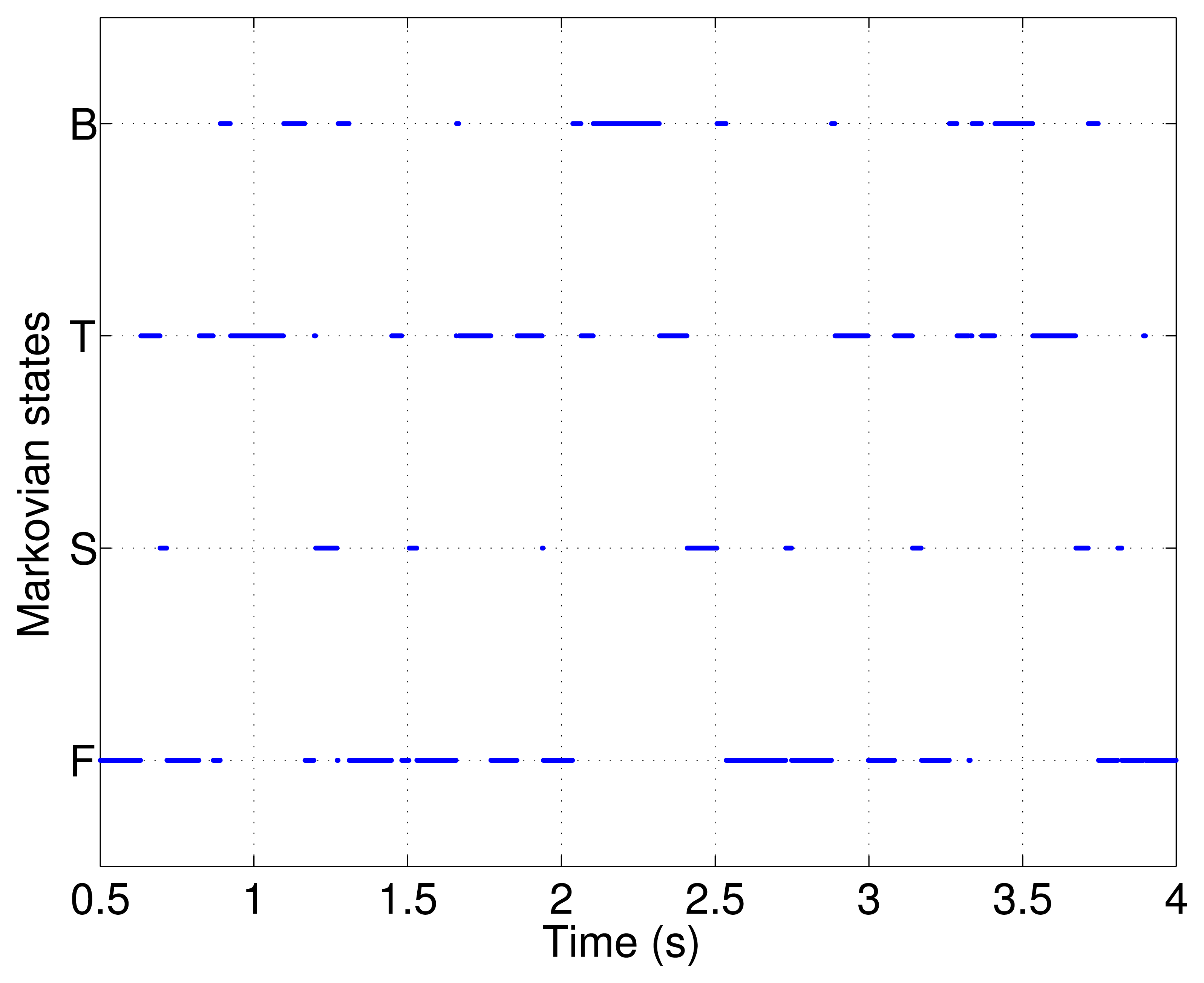
Figure 3a shows the four Markovian states (B, Body; T, Thigh; S, Shank; F, Foot) of the proposed MJLS model. They are defined as the condition where the related IMU presents the smallest dynamic acceleration. In Figure 3b, we show the time intervals where each IMU reaches the Markovian states condition for one step. The incidence of dynamic accelerations is evaluated by computing the acceleration vector module, which includes all accelerometer axes. They are compared, in turn, to the gravitational acceleration.
The MJLS model for angular position estimation of lower limbs exoskeletons can be described by the following state-space equations:
Considering the gyroscope, accelerometer and gyroscope bias models, matrices Ᾱ and C̄ are defined as:
In the proposed approach, only one inertial sensor is used at each instant in combination with three relative sensors. As the system has four inertial sensors, the Markovian model presents four states, as shown in Figure 3a.
In Equation (18), four variables, MB(t), MT(t), MS(t) and MF(t), select the inertial sensor, which will be used at each time instant. Table 1 presents the Markovian states and the related variable values.
After generating the estimation errors for all angles from the Markovian filter, the estimated absolute angles are given by:
3. Implementing
In this section, we present the Markovian Kalman filter (MKF) and the guidelines to choose the Markovian states for each instant of time. Consider the discrete-time version of the Markovian model, described in Section 2.3, given by:
Predicting equations:
Updating equations:
where the weighting matrix, Q, is time-invariant and given by:
On the other hand, the weighting matrix, R, is considered time-variant, since it changes according to the Markov chain. It is given by:
Required Conditions to Apply the Filter
The reliability of the accelerometer signal is essential to define the current Markovian state, in order to be used in the Kalman filter. When the module of the triaxial accelerometer vector is near the module of the gravity vector, there exists a low incidence of dynamic accelerations. We can define that the current incidence of dynamic accelerations and the Markovian state are chosen as:
Thereby, the general condition to verify the reliability of the current IMU reading is given by:
Let the magnitude vector measured by the four IMUs attached in a lower limbs exoskeleton (see Figure 2), for k = 1 to 10, be given by:
Then, applying Equations (28) and (29), we obtain:
Notice that we have two possible alternatives:
Reliable measurement signal: In this case, the proposed MKF performs the prediction and update of the estimated angle, Equations (21) to (25).
Unreliable measurement signal: In this case, the MKF performs only the prediction, Equations (21) and (22). The estimated angle is not corrected by the accelerometer measurement.
4. Results and Discussion
In order to present the simulation results, we consider the following assumptions:
The angular estimate is performed for one leg of the exoskeleton (trunk to foot; see Figure 2).
In the standard case, modeled in Section 2.2, the system is replicated for each segment of the exoskeleton. More details on the implementation of the standard Kalman filter can be seen in [8].
In the Markovian case, modeled in Section 2.3, all segments are included in a unified model.
For both estimate approaches, the weighting matrices parameters are given in Table 2. They were obtained based on optimization procedure given in [8].
As discussed in Section 3, to define the sequence of Markov jumps among B, T, S and F, Equation (30) was used. The Markov chain was considered for three steps (see Figure 4).
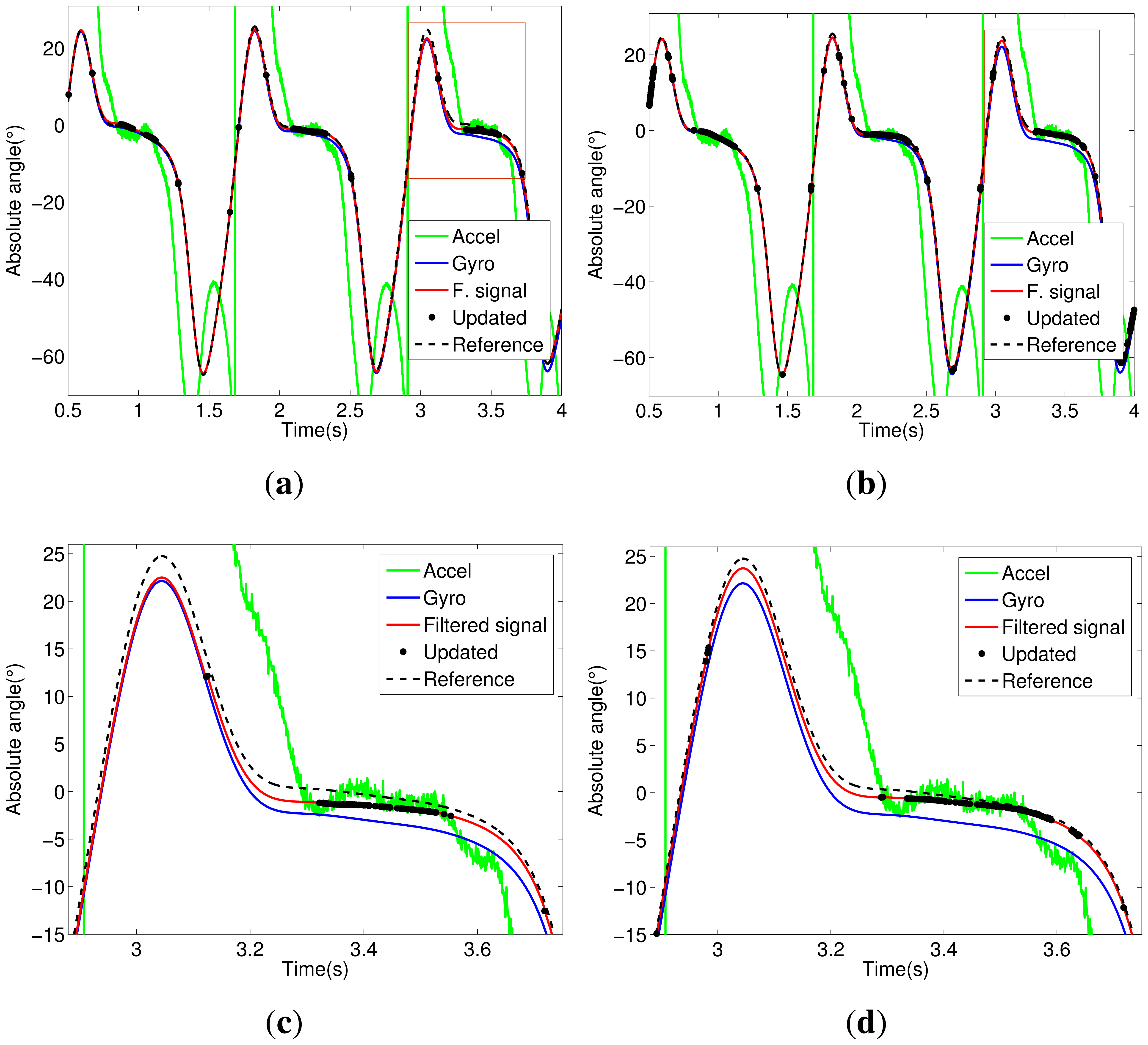
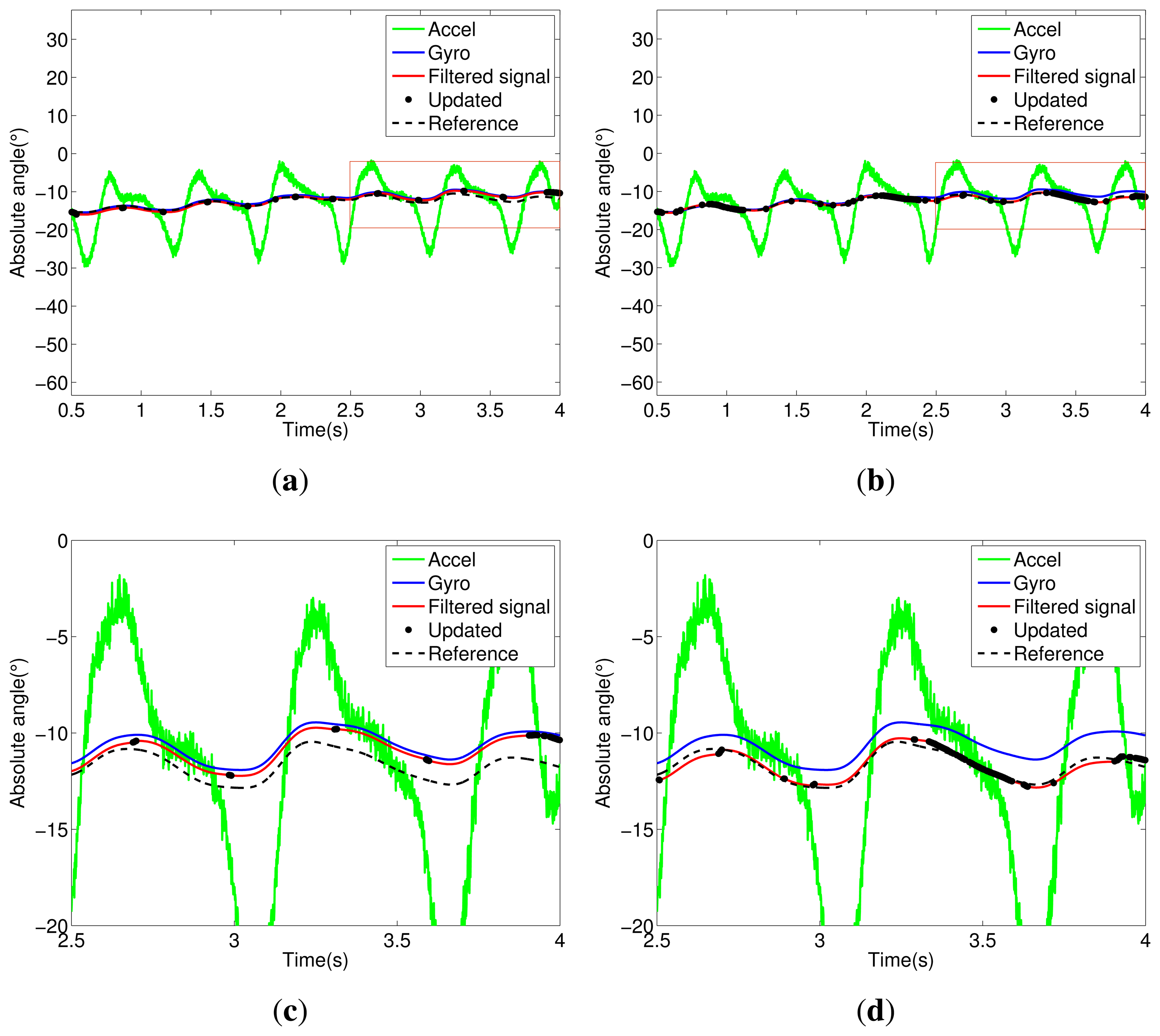
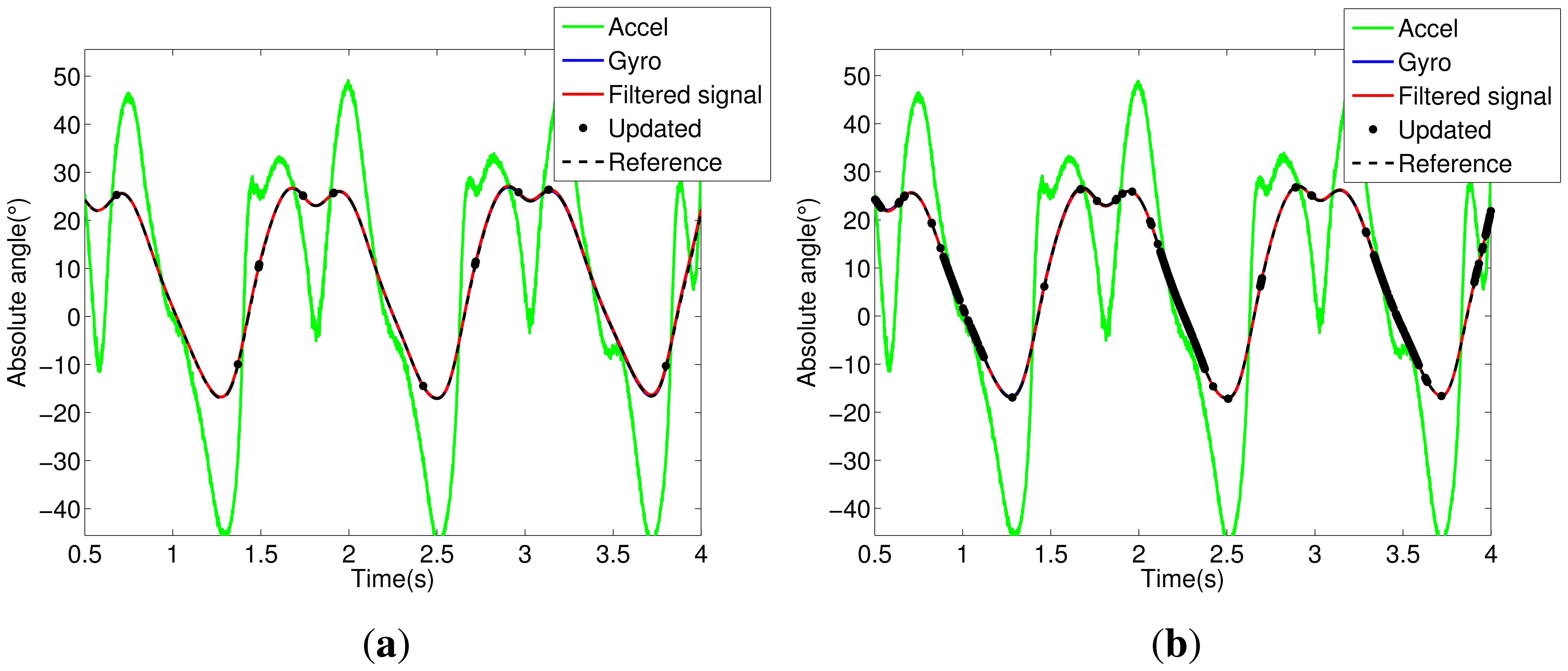
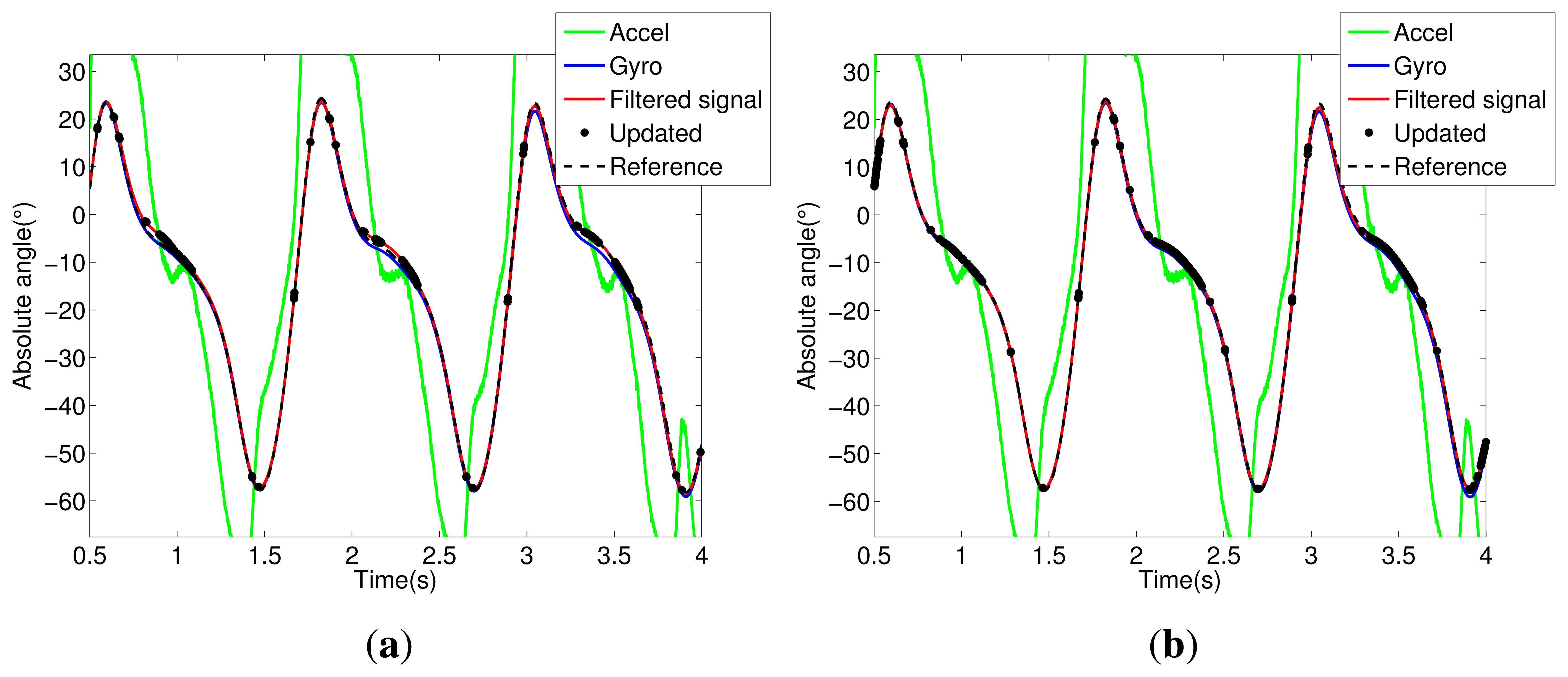
Notice in Figure 5 that the trunk segment features have the most critical condition for angular estimation. It presents large dynamic acceleration levels cumulatively from the other segments (thigh, shank and foot) in all stages of walking. Thus, the accelerometer attached to the trunk has a reliable signal only for a few intervals; see the updated signals shown in Figure 5c. In Figure 5d, we can see the influence of the Markovian approach, which decreases the estimation error between filtered and reference signals. The same analysis can be extended to other segments of the exoskeleton, shown in Figures 5, 6, 7 and 8.
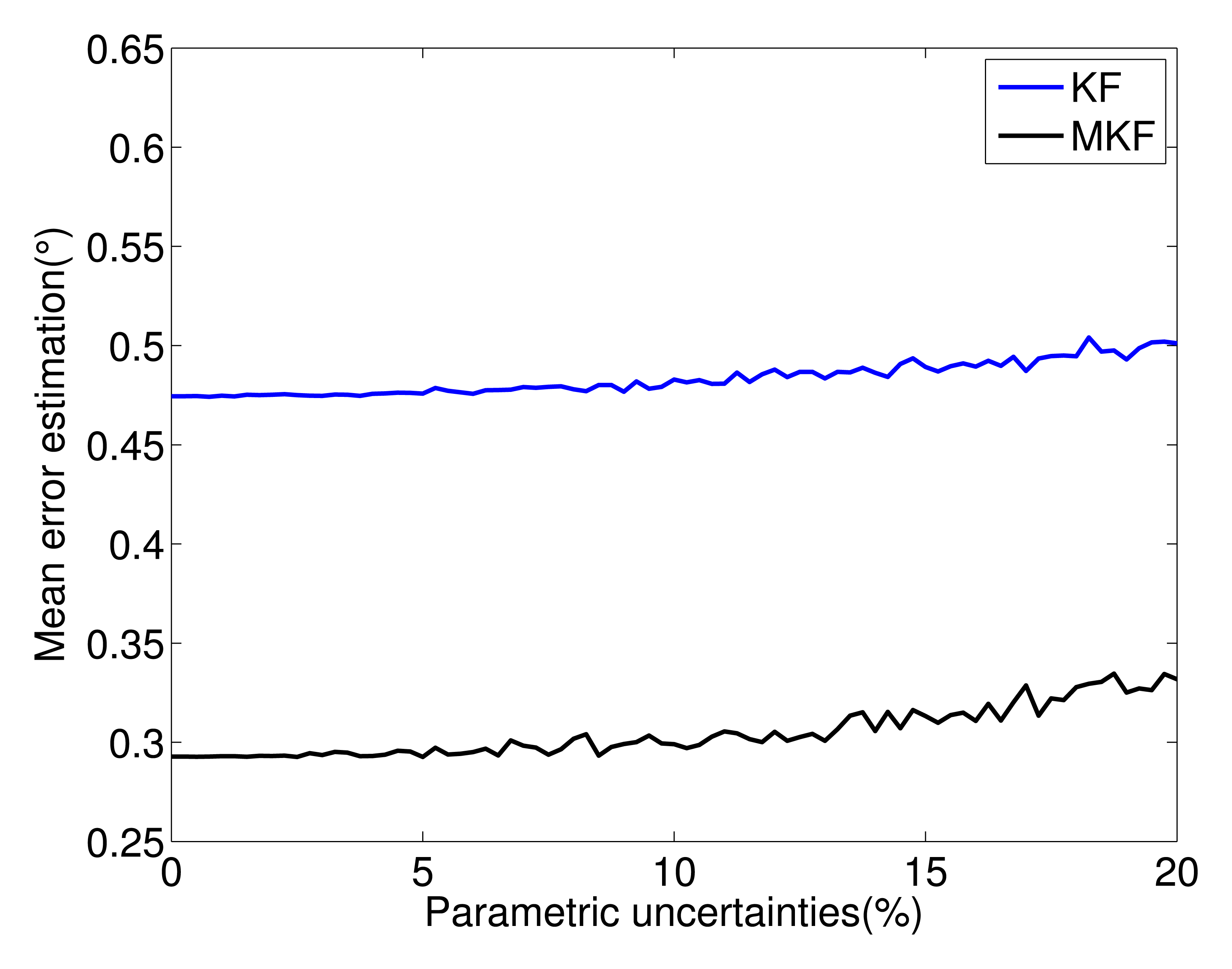
In order to verify the effectiveness of the filters when the system is subject to parametric uncertainties, both estimators were run, varying the components of the system matrices. Variations from 0% to 20% are assumed in the nominal values. Furthermore, 100 Monte Carlo simulations were performed. In Figure 9 are shown the estimation mean error for each filter. Notice the better performance of the Markovian approach over the standard Kalman filter for all ranges of uncertainties.
5. Conclusions
A MJLS-based position estimation approach for lower limbs exoskeletons is presented in this paper. Unlike the standard position estimations, where inertial sensors are designed to work individually for each link, the proposed approach considers a collective modeling of all inertial sensors attached to the exoskeleton. They are combined in a Markovian estimation model. Simulations results were presented considering the kinematic model of an exoskeleton for lower limbs, where four IMUs and three encoders were used. The results show the advantage of the proposed Markovian estimation model if compared with the standard one, even when they are subject to a wide range of parametric uncertainties.
Acknowledgments
This work was supported by Coordenação de Aperfeiçoamento de Pessoal de Nível Superior (CAPES) and Fundação de Apoio à Pesquisa do Estado de São Paulo (FAPESP), under grant 2012/05552-9.
Conflicts of Interest
The authors declare no conflict of interest.
References
- Blaya, J.B. Force Controllable Ankle-Foot Orthosis (AFO) to Assist Drop Foot Gait. Master's Thesis, Massachusetts Institute of Technology, Cambridge, MA, USA, 2002. [Google Scholar]
- Pons, J.; Moreno, J.; Brunetti, F.; Roccon, E. Lower-Limb Wearable Exoskeleton; Rehabilitation Robotics: Vienna, Austria, 2007. [Google Scholar]
- Frisoli, A.; Procopio, C.; Chisari, C.; Creatini, I.; Bonfiglio, L.; Bergamasco, M.; Rossi, B.; Carboncini, M. Positive effects of robotic exoskeleton training of upper limb reaching movements after stroke. J. NeuroEng. Rehabil. 2012, 9, 36. [Google Scholar]
- Tong, K.; Granat, M.H. A practical gait analysis system using gyroscopes. Med. Eng. Phys. 1999, 21, 87–94. [Google Scholar]
- Lau, H.; Tong, K. The reliability of using accelerometer and gyroscope for gait event identification on persons with dropped foot. Gait Posture 2008, 27, 248–257. [Google Scholar]
- Moreno, J.C.; de Lima, E.R.; Ruíz, A.F.; Brunetti, F.J.; Pons, J.L. Design and implementation of an inertial measurement unit for control of artificial limbs: Application on leg orthoses. Sens. Actuators B Chem. 2006, 118, 333–337. [Google Scholar]
- Pappas, I.; Keller, T.; Mangold, S.; Popovic, M.; Dietz, V.; Morari, M. A reliable gyroscope-based gait-phase detection sensor embedded in a shoe insole. IEEE Sens. J. 2004, 4, 268–274. [Google Scholar]
- Nogueira, S.L.; Inoue, R.S.; Terra, M.H.; Siqueira, A.A.G. Estimation of Lower Limbs Angular Positions Using Kalman Filter and Genetic Algorithm. 1–6.
- Nogueira, S.L.; Siqueira, A.A.G.; Inoue, R.S.; Terra, M.H. Estimation of Lower Limbs Angular Positions Using Robst Kalman Filter and Genetic Algorithm. Proceedings of the 22nd International Congress of Mechanical Engineering, Ribeirao Preto, Brazil, 3–7 November 2013.
- Siqueira, A.A.G.; Terra, M.H. Nonlinear and Markovian
![Sensors 14 01835 g01]() ∞ controls of underactuated manipulators. IEEE Trans. Control Syst. Technol. 2004, 12, 811–826. [Google Scholar]
∞ controls of underactuated manipulators. IEEE Trans. Control Syst. Technol. 2004, 12, 811–826. [Google Scholar] - Chizeck, H.; Ji, Y. Optimal Quadratic Control of Jump Linear Systems with Gaussian Noise in Discrete-Time. Proceedings of the 27th IEEE Conference on Decision and Control, Austin, TX, USA, 7–9 December 1988; Volume 3, pp. 1989–1993.


| Modes of Operation (Θ(t)) | MB(t) | MT(t) | MS(t) | MF(t) |
|---|---|---|---|---|
| B | 1 | 0 | 0 | 0 |
| T | 0 | 1 | 0 | 0 |
| S | 0 | 0 | 1 | 0 |
| F | 0 | 0 | 0 | 1 |
| KF | ζ | σg | σbg | σa | τg |
|---|---|---|---|---|---|
| Body/Trunk | 0.01 | 0.0103 | 0.0003 | 46.562 | 839.70 |
| Thigh | 0.01 | 0.0017 | 0.0005 | 329.08 | 2138.5 |
| Shank | 0.01 | 0.0008 | 9.6405 | 100.94 | 1465.3 |
| Foot | 0.01 | 7.7482 | 18.594 | 291.29 | 3567.5 |
© 2014 by the authors; licensee MDPI, Basel, Switzerland. This article is an open access article distributed under the terms and conditions of the Creative Commons Attribution license (http://creativecommons.org/licenses/by/3.0/).
Share and Cite
Nogueira, S.L.; Siqueira, A.A.G.; Inoue, R.S.; Terra, M.H. Markov Jump Linear Systems-Based Position Estimation for Lower Limb Exoskeletons. Sensors 2014, 14, 1835-1849. https://doi.org/10.3390/s140101835
Nogueira SL, Siqueira AAG, Inoue RS, Terra MH. Markov Jump Linear Systems-Based Position Estimation for Lower Limb Exoskeletons. Sensors. 2014; 14(1):1835-1849. https://doi.org/10.3390/s140101835
Chicago/Turabian StyleNogueira, Samuel L., Adriano A. G. Siqueira, Roberto S. Inoue, and Marco H. Terra. 2014. "Markov Jump Linear Systems-Based Position Estimation for Lower Limb Exoskeletons" Sensors 14, no. 1: 1835-1849. https://doi.org/10.3390/s140101835