Metal Oxide Gas Sensor Drift Compensation Using a Dynamic Classifier Ensemble Based on Fitting

Abstract
: Sensor drift is currently the most challenging problem in gas sensing. We propose a novel ensemble method with dynamic weights based on fitting (DWF) to solve the gas discrimination problem, regardless of the gas concentration, with high accuracy over extended periods of time. The DWF method uses a dynamic weighted combination of support vector machine (SVM) classifiers trained by the datasets that are collected at different time periods. In the testing of future datasets, the classifier weights are predicted by fitting functions, which are obtained by the proper fitting of the optimal weights during training. We compare the performance of the DWF method with that of competing methods in an experiment based on a public dataset that was compiled over a period of three years. The experimental results demonstrate that the DWF method outperforms the other methods considered. Furthermore, the DWF method can be further optimized by applying a fitting function that more closely matches the variation of the optimal weight over time.1. Introduction
Electronic noses, a collection of broadly cross-reactive sensors connected to electronics and an effective pattern recognition system, are used to detect, classify and, where necessary, quantify a variety of chemical analytes or odors of concern in the area of interest [1]. The key issue in construction of such systems is the selection and stability of sensors. A phenomenon known as sensor drift has been recognized as one of the most serious impairments of the above performance [2].
Romain and co-workers systematically analyzed sensor drift [3]. They utilized a very comprehensive dataset, collected over a period of three years under real operating conditions [4], to provide further insight into the sensor drift problem with regard to both first- and second-order drift. In this paper, we focus exclusively on the first-order drift (hereafter referred to as “drift”) of the metal oxide sensor.
There are several different ways of drift reduction, which can be classified into three main categories. The first is the search for new materials that can reversibly interact with the relevant gas, so that the detected molecules unbind from the sensor material as soon as the gas has been purged from the sensor surface [5,6]. The second is the dynamical characterization of the sensor response. Some solutions based on periodically changing the working temperature of the sensor [7,8] have been implemented to minimize the effects of irreversibility in the sensor response due to poisoning. Additionally, the third is the use of sensor arrays and appropriate signal processing techniques, including feature extraction and pattern recognition techniques.
Note that the research of this paper is based on an assumption that all sensors function correctly. Sensor failure, which is another type of sensor degradation, has also attracted great attention. Pattern recognition techniques are also used to detect faults, such as [9–11].
This paper focuses on the gas discrimination using metal oxide gas sensor array, regardless of the gas concentration. Under the condition of other unchanged factors, such as sensor materials and number, environment, feature extraction methods, etc., the influence of the sensor drift on discrimination is avoided or reduced over longer periods of time, just by improving the classification method. A classifier ensemble method with dynamic weights based on fitting (DWF) is proposed in this paper. Experimental results indicate that the performance of the DWF degrades more slowly over time than that of the static classifier ensembles. The DWF can mitigate the drift effect in metal oxide gas sensors for a longer period of time, thereby prolonging the lifetime of metal oxide gas sensors.
In the remainder of this paper, we first survey the existing work by the chemical sensing community on the problem of using classifier methods (Section 2). Next, the DWF method proposed in this paper is described (Section 3), and this is followed by a detailed description of the experiment (Section 4). Finally, the conclusions drawn from the results presented in this paper are presented (Section 5).
2. Related Work
In the early days, analytes were identified by a single classifier model, such as support vector machine (SVM), artificial neural network (ANN) and their derivatives. Lee et al. used a multi-layer neural network with an error back propagation learning algorithm as a gas pattern recognizer [12]. Polikar et al. used a neural network classifier and employed the hill-climb search algorithm to maximize the performance [13]. The authors in [14–17] also used ANN to identify the analytes of interest. Xu et al. used a Fuzzy ARTMAPclassifier, which is a constructive neural network model developed upon adaptive resonance theory (ART) and fuzzy set theory [18]. Some other researchers used SVM to solve classification in E-nose signal processing, such as [19–21].
The ensemble-based method is becoming an increasingly important method in the chemical sensing research community. An ensemble-based method trains a base classifier on each batch of datasets, followed by the construction of an ensemble of the base classifiers that are used to predict the testing dataset. Compared to using a single classifier model for prediction, classifier ensemble methods have been found to improve the performance, provided that the base models are sufficiently accurate and diverse in their predictions [22].
The methods of integrating base classifiers can be divided into two categories: static classifier ensembles and dynamic classifier ensembles. In a static classifier ensemble, the weight of each base classifier is decided before the classification phase. In a dynamic classifier ensemble, the weight of each base classifier is decided dynamically during the classification phase. Gao et al. used an ensemble of multilayer perceptions (MLPs), which are feedforward artificial neural network models [23], and that of four base models (namely MLP, MVLR, QMVLRand SVM) [24] to predict, simultaneously, both the classes and concentrations of odors. Shi et al. proposed an ensemble of density models, KNN, ANN and SVM, for odor discrimination [25]. Vergara et al. used a static ensemble of multiple SVMs to cope with the problem of drift in chemical gas sensors [26]. Wang et al. also proposed a static ensemble of SVMs, which is similar to that of Vergara et al., only instead of the weight assignment method [27]. Amini et al. used an ensemble of SVMs or MLPs on data from a single metal oxide gas sensor (SP3-AQ2, FIS Inc., Hyogo, Japan) operated at six different rectangular heating voltage pulses (temperature modulation), to identify analytes regardless of concentration [28]. The experimental result showed that the accuracies obtained with the ensembles of SVMs or MLPs were almost equal, if using an identical integrating method. Very recently, Kadri et al. proposed a dynamic ensemble method called dynamic weighting of base models (DWBM) just for concentration estimation of some indoor air pollutants [29].
The performance of all ensemble methods described above degrade over time due to drift. Predictably, the performance of future ensemble methods will also degrade inevitably, if drift still exist. In the next section, we describe a novel ensemble method with dynamic weights based on fitting (DWF) to achieve improved performance (or to minimize degradation) over time.
3. Dynamic Classifier Ensemble and Predictions
3.1. The Problem of Static Classifier Ensembles
Consider a classification problem with a set of features, x, as the inputs and a class label (a gas/analyte in our problem), y, as the output. At every time step, t, a batch of examples, St = (Xt, Yt) = {(x1, y1), …, (xmt, ymt)}, of size, mt, is received. A classifier model, ft(x), is trained on the dataset, St. If S1–T (namely, St, t = 1, …, T) are training datasets, the classifier ensemble, hT(x), is a weighted combination of the classifiers trained on S1–T, respectively, i.e., , where {β1, …, βT } is the set of classifier weights. The ensemble method in its most general form is described in Algorithm 1. The remaining problem is how to estimate the optimal weights.
A common and intuitive method to estimate the weights is to assign weights to the classifiers according to their prediction performance on batch ST, e.g., [26]. Wang et al.[27] use the weight, βi = MSEr – MSEi, for each classifier, fi, where MSEi is the mean square error of classifier fi on ST and MSEr is the mean square error of a classifier predicting randomly.
| Algorithm 1 The classifier ensemble method in its most general form. | |
| Require: Datasets St = {(x1, y1), …, (xmt, ymt)}, t = 1, …, T. | |
| 1: | for t = 1, …, T do |
| 2: | Train the classifier, ft on St; |
| 3: | Estimate the weight, βt, of ft using dataset ST by the appropriate technique; |
| 4: | end for |
| 5: | Normalize the weights, {β1, …, βT}; |
| Ensure: A set of classifiers, {f1, …, fT}, and corresponding weights, {β1, …, βT}. | |
To evaluate the performance of the ensembles, which use the weights estimated by the existing methods, the following experiment is carried out. The data used in this experiment was gathered by Vergara et al. [26]. They used 16 screen-printed MOXgas sensors (TGS2600, TGS2602, TGS2610 and TGS2620, four of each type) commercialized and manufactured by Figaro Inc. The resulting dataset comprises 13,910 recordings of the 16-sensor array when exposed to six distinct pure gaseous substances, namely, ammonia, acetaldehyde, acetone, ethylene, ethanol and toluene, each dosed in a wide variety of concentration values, ranging from 5 to 1,000 ppmv They map the sensor array response into a 128-dimensional feature vector, which resulted from a combination of the eight features described in [30] × 16 sensors. The measurements collected over the 36-month period are combined to form 10 batches, such that the number of measurements is as uniformly distributed as possible.
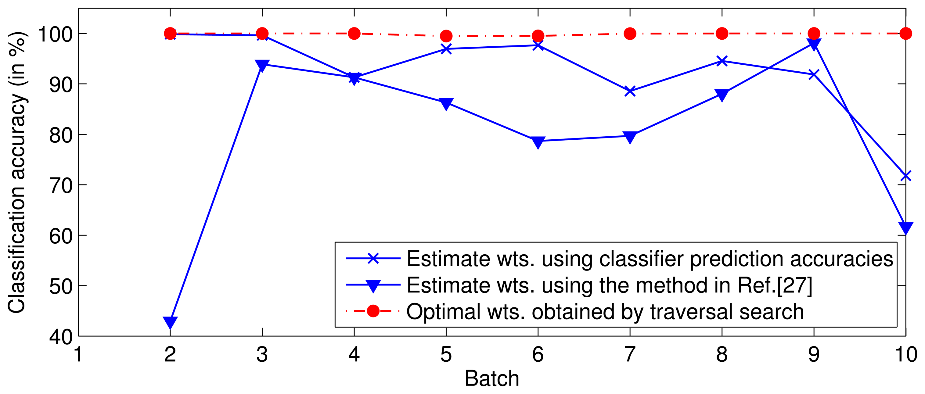
In the experiment, for a given T, a set of classifiers (SVMs), f1, …, fT, are trained on batches S1, …, ST, respectively. Next, ST+1 is predicted by the ensemble of classifiers, f1, …, fT, with the optimal weights or the weights estimated by the above-mentioned methods. The optimal weights are obtained by a traversal search. The experimental result (Figure 1) indicates that the performance with the optimal weights is superior to that with the estimated weights, i.e., the weights estimated by the existing methods are not optimal.
Most classifier ensemble methods, such as those described in references [26,27], are proposed based on an assumption that the distribution of the examples in the following batch, ST+1, does not change significantly from that in the current batch, ST. Thus, these methods use the examples in batch ST to estimate the weights, {β1, …, βT }, for ST+1. In other words, they use static weights for the following batches, ST+1, ST+2,…. For ST+n, if n is too large, i.e., the time gap between time step T and T + n is too large, the relative drift may noticeably influence the prediction performance of the ensemble at T + n, of which the weights are estimated by some parameters of the ensemble at T.
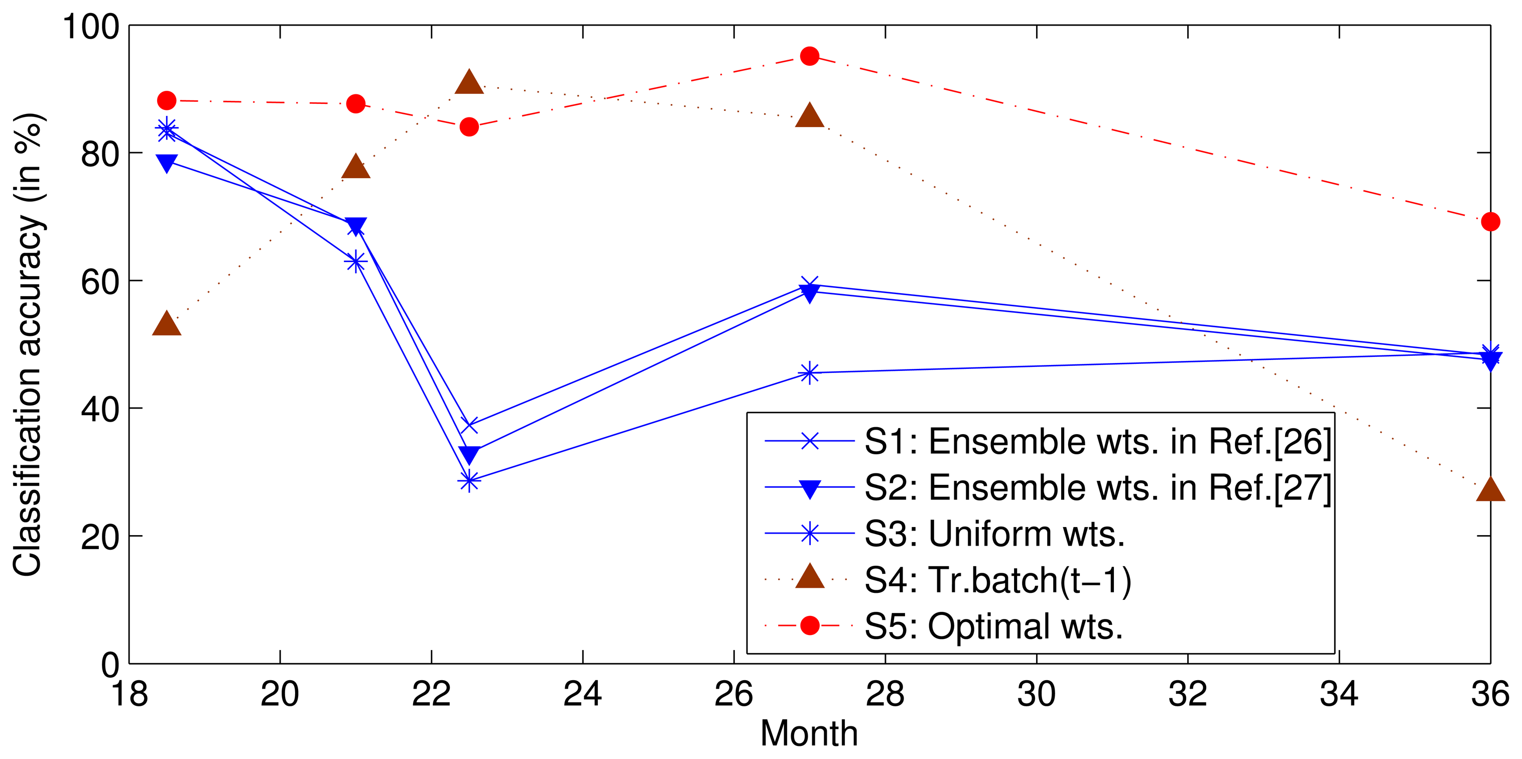
To survey the influence of the relative drift, we used the same data and features as those used in a previous study [26] to complete the following experiment. We trained SVMs on batches S1–5 and then tested batches S6–10 using uniform weights (Setting 3) or a set of weights estimated using batch S5 with the methods proposed in [26,27] (Setting 1 and 2). To determine the best prediction performance of ensemble f1–5, we determined the traversal search sets of the optimal weights for each classifier in batches S6–10 (Setting 5); the ensemble classifier was found to perform with the greatest accuracy where the search range for each weight was [0,1] and the search step was 0.01, due to calculating time pressure. In addition, to verify the above assumption, we trained a classifier with data from only the previous batch and tested it on the current batch (Setting 4). The classification accuracies are shown in Figure 2, where the horizontal axis represents the mean time at which the data for each batch was collected. Note that the performance under Setting 4 is typically not the best. This non-ideal performance illustrates that the ensemble of the earlier SVMs with advisable weights can perform better than the SVM trained by only the previous batch. The optimal weights for each batch are obtained under Setting 5, and the performance is theoretically the best that can be obtained by class ensembles when {X1–5, Y1–5} and X6–10 are known and Y6–10 are unknown.
Predicting the optimal weight of each classifier for the incoming batch is difficult or impossible. The objective of this study is to predict the near-optimal weights. The performance under Settings 1 to 3 is close to the optimal performance (Setting 5) in the initial stages, but the performance degrades over time. This performance indicates that the near optimal weights can be obtained by using static weights, but the performance degrades with an increasing gap between the training dataset and test dataset. Because of this gap, a dynamic ensemble classifier is proposed in this paper to delay the degradation of performance and extend the life of the sensor.
3.2. Proposed Method
The performance of classifier ensembles with static weights degrades over time due to drift. To address this drift, a novel ensemble method with dynamic weights based on fitting (DWF), which is described below in its general form, is proposed in this paper to achieve improved performance (or to minimize degradation) over time.
We define T as the index of the current time step, and all sets of features, Xt, and their class labels, Yt, in each batch, St, t ≤ T, have been know, where t is the index of the time step. Thus, the dataset, Xt, t ≤ T, can be predicted by the classifiers trained on not only the prior batch, Si, i < t, but also the later batch, Sj, j > t. After training the classifiers on each batch, some classifiers, ft, t ≤ T, are received. All of the classifier ensembles are the weighted combinations of these classifiers.
At this point, the first important problem encountered is how to obtain the optimal or suboptimal weight of ft for each training batch. The experiment (Figure 1) has confirmed that the accuracies of the existing methods are much worse than the theoretical optimum accuracy. In this paper, we used a traversal search approach to determine the optimal weights of fi, i = 1, …, T, for each training batch, Sj, j ≤ T. The search range for each weight is [0,1], and the search step is set to 0.05, due to the calculating time pressure. Table 1 lists the optimal weights of each classifier when T = 5. The use of the traversal search method can ensure that all of the weights are optimal, but the calculation requires a significant amount of time. The optimal weight matrix, namely, in the DWF method, consists of the weight of each classifier, fi, for training batch Sj. The row vector of the matrix, , is the subset of the optimal weights of the classifier at different time steps, and the column vector of that is the optimal weights assigned to all the classifiers at the corresponding time step. If scaling a column vector of , the performance of the ensemble will stay invariable at the corresponding time step, because the proportion between the weights of the base classifiers do not change, which determines the performance, in fact. Thus, in the fitting stage, the curve of one classifier is fitted first. Then, the scaling factor of each column vector can be determined by the curve, i.e., the 8th and 9th procedures in Algorithm 2-1.
| Algorithm 2 DWF method | |
| (2-1) The training and fitting stages. | |
| Require: Training datasets, St = {(x1, y1), …, (xmt, ymt)}, t = 1, …, T, and the mean measurement time, wt, of each dataset. | |
| 1: | for t = 1, …, T do |
| 2: | Train a classifier, ft, on St; |
| 3: | end for |
| 4: | for t = 1, …, T do |
| 5: | Estimate the optimal weights, { ,… }, of {f1, …, fT} for St using the appropriate technique; |
| 6: | end for |
| 7: | Receive a T × T matrix, ; |
| 8: | For a classifier, i.e., ft0, fit curve, Ct0(w), with {( , ω1), …, ( , ωT)}; |
| 9: | Revise the t0th row vector, βt0, as [Ct0(w1), …, Ct0(wT)], by means of scaling each column vector of ; |
| 10: | for t = 1, …, T except t0 do |
| 11: | Fit curve Ct(w) with {( , w1), …, ( , wT)}; |
| 12: | end for |
| Ensure: The classifiers, ft, and the corresponding fitting functions, Ct(w), t = 1, …, T. | |
| (2-2) The testing stage. | |
| Require: Test the dataset, XT+n, and the mean measurement time, wT+n, n > 0; the classifiers, ft, and the corresponding fitting functions, Ct(w), t = 1, …, T. | |
| 1: | for t = 1, …, T do |
| 2: | Calculate the weight of ft at time wT+n, namely Ct(wT+n); |
| 3: | end for |
| 4: | Test XT+n using the classifier ensemble, ; |
| 5: | Estimate the labels: YT+n = hT+n(XT+n); |
| Ensure: Estimated labels YT+n. | |
From , the optimal weight of a classifier is observed to change over time. The weight of fi for a training batch, Sj, and the corresponding mean measurement time of the batch form a two-dimensional array, ( , wj). All of the arrays about fi, namely, {( , w1), …, ( , wT)}, can be used to fit a weight curve, Ci(w), that is a function of time, w, for the classifier, fi, where wj is real time corresponding to index j. The weight of fi at time, wT+n, n = 1,2, …, can be predicted as Ci(wT+n).
At this point, the second important problem encountered is determining what function can be used to fit these curves. Table 1 illustrates that, for most classifiers, the weight of fi is the maximum of all of the classifier weights at time step i, and the weight degrades from i to earlier or later. Thus, the fitting function, Ci(w), should satisfy the following conditions: (I) Ci(w) has maximum value at wi ; (II) Ci(w1) – Ci(w2) > 0 if w2 < w1 < wi or w2 > w1 > wi; (III) Ci(w) > 0. Thus, the following function is proposed to fit the weight curve of the base classifier in this paper:
After fitting, four parameters (a, b, c and d) are determined for each function, Ci(w), i = 1, …, T.
It should be noted that, scaling a column vector of does not change the accuracy of the classifier ensemble at the corresponding time step; however, it significantly affects the profile of each fit curve. Thus, a normalizing method is proposed for in the fitting stage. At first, a classifier, i.e., ft0, is chosen, and its curve, Ct0(w), is fitted by the t0th row vector of and the corresponding time, namely, {( , w1), …, ( , wT)}. Then, scale each column vector of , such that its t0th row vector is [Ct0(w1), …, Ct0(wT)]. Table 2 shows the normalized that is more conforming to the characteristics of the fitting function.
In the test stage, if the test dataset is XT+n, n > 0, the weight of each classifier, fi, at time step T + n is Ci(wT+n). Thus, the final classifier ensemble at time step (T + n) is a weighted combination of these classifiers, namely:
The predicted label set of XT+n is:
4. Experimental Section
In all our experiments, we train the multi-class SVMs (one-vs.-one strategy) with the RBFkernel using the publicly available LibSVM software. The datasets used in Section 3.1 are also used in the experiments. Because the dataset for toluene is lacking for almost one year, we test only the remaining five analytes.
At least four fitting points are required to calculate the four parameters in the fitting function. Thus, the datasets used in the training stage must be no less than 4 batches and, preferably, many more batches. On the other hand, the DWF method is proposed to mitigate the drift effect for a longer period of time, so enough batches of datasets are expected in the testing stage. Considering only 10 batches of datasets can be used in the training and testing stages, four ways of partitioning datasets are set up to compare the performance of the DWF with that of recent methods.
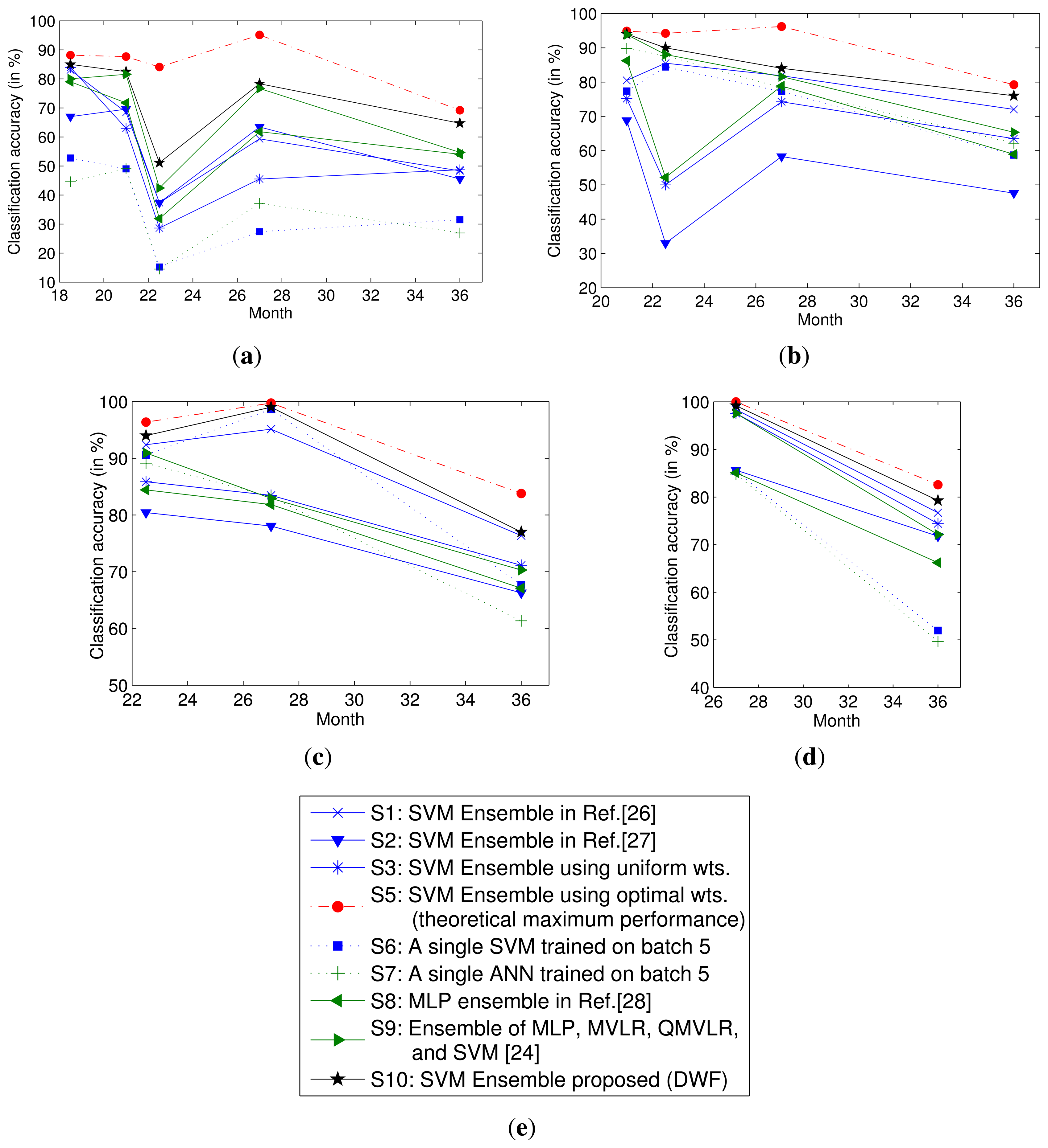
The parameters of the five fitting functions are provided in Table 3, and the predicted weights of each classifier at time t ≥ 6 are provided in Table 4. The performance of the DWF method proposed in this paper is illustrated in Figure 3. For comparison, Figure 3 also illustrates the performance under other settings. Settings 1–3 are the same as those used in Figure 2. The theoretical maximum performance using the SVM ensemble is illustrated under Setting 5. Under Setting 6 and 7, an SVM and an ANN model are trained on the most recent training batch, respectively. Their performances are strong baselines, because the batch used in training is corrupted least by the drifted data from the past. Under Setting 8, an MLP ensemble [28] is used, and under Setting 9, an ensemble of four base models (namely MLP, MVLR, QMVLR and SVM) [24] is used. The performance of the DWF method is illustrated under Setting 10.
Experimental results show that the classifier using a single model depends heavily on selecting the training batch. In the classifier ensembles, the DWF method outperforms the other methods considered at all times. The ensemble under Setting 9 performs slightly worse than DWF. The performances under Settings 1, 2 and 8 are relatively close. Additionally, the performance under Setting 3 is worst at some time steps. All the performances degrade over time, but the performance of the DWF degrades more slowly over time than that of others. Therefore, it can be concluded that the DWF can mitigate the drift effect in metal oxide gas sensors for a longer period of time, thereby prolonging the lifetime of metal oxide gas sensors.
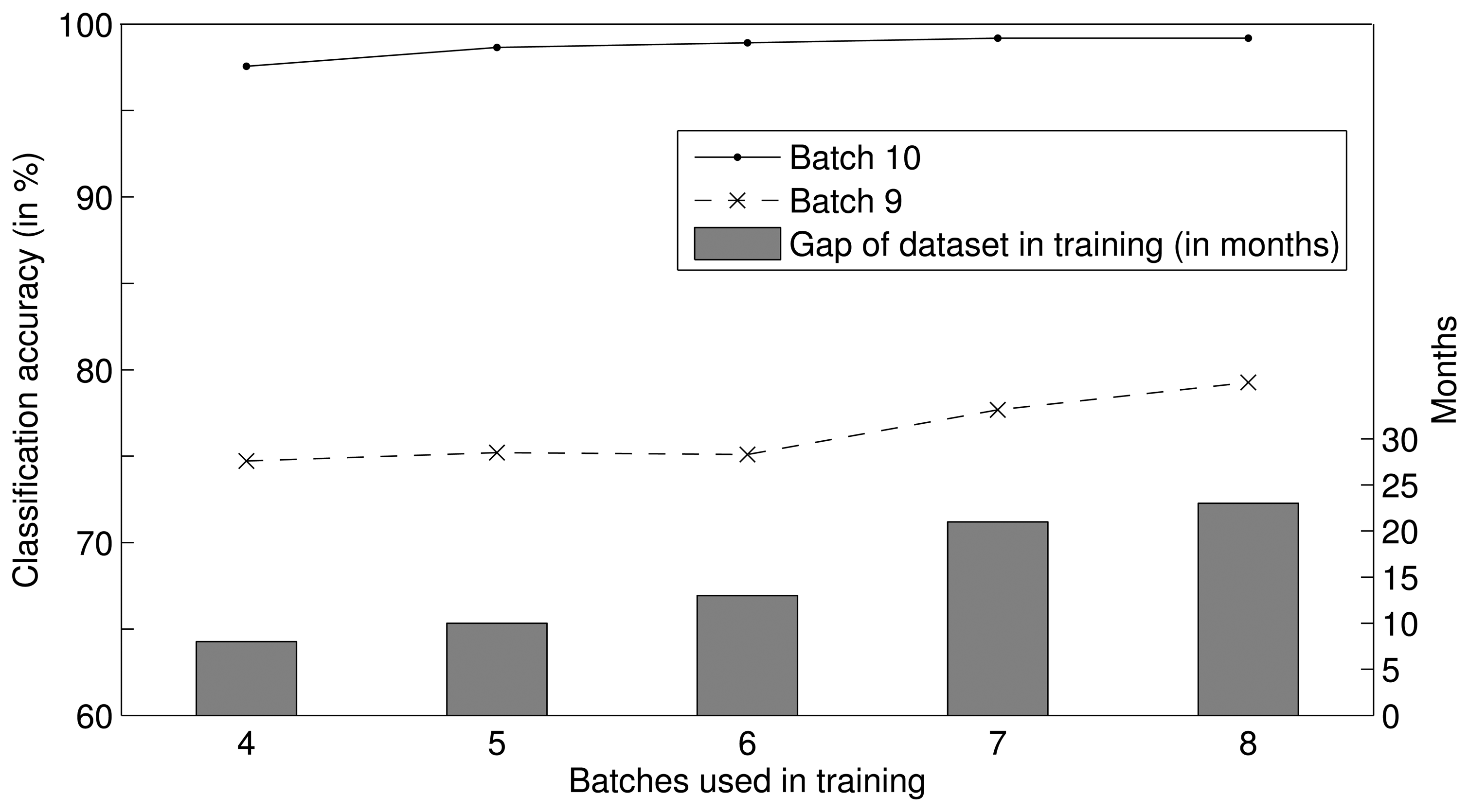
In the DWF approach, the weights in the test step are predicted by fitting functions, and the time span of the training dataset can affect the fitting result. It follows that the time span of the training dataset can affect the performance of the DWF approach. To verify this inference, we analyzed the impact of the time span on the classification accuracy in a set of experiments. We trained sets of SVMs using the datasets of different time spans for batches S5–8, S4–8, S3–8, S2–8, and S1–8, and combined five classifier ensembles, which are composed of four, five, six, seven and eight SVMs, respectively. Then, based on the DWF method, we predicted the weight of each SVM at the times of batches S9 and S10 and tested these predictions. Figure 4 illustrates the performance of each ensemble, where the histogram presents the time span of the training datasets of each ensemble, and the two profiles illustrate the classification accuracies of each ensemble tested on batches S9 and S10. The classification accuracies were found to increase as the time span of the training dataset increased, and the classification accuracy increased more substantially as the time gap between the training and test datasets increased. In conclusion, the performance of the DWF method can be improved by increasing the time span of the training dataset; in other words, the DWF approach can mitigate the drift effect for a longer period of time when the time span of the training dataset is increased.
5. Conclusions
This paper proposes a DWF method to mitigate the drift effect in metal oxide gas sensors. The experimental results indicate that the DWF method is able to cope well with sensor drift and perform better than the competing static-weighted ensemble methods. There are two vital problems in the DWF method. One problem involves the method for estimating the optimal weights in the training stage. For simplicity, the classifier prediction accuracy on recent training batches is commonly used to estimate the weights, but the experimental results confirm that the weights obtained by this method are not optimal. The performance of the ensemble assigning weights according to their prediction performances is much worse than that using weights obtained by the traversal search approach (Figure 1). However, the traversal search is too slow to be used in practice, so a novel solution is required to estimate the optimal weights. The other problem involves the selection of the fitting function. DWF relies on the proper selection of the fitting function. The curve features of the function should match the variation of the optimal weight over time. Besides, a fitting function with fewer parameters is expected. A further study will be performed to address these two problems.
Acknowledgments
This work has been supported by the Fundamental Research Funds for the Central Universities (Grant No. DUT11RC(3)74) and the National Natural Science Foundation of China (Grant No. 61131004). The authors thank Vergara et al. for publishing the comprehensive dataset over a period of three years.
Conflict of Interest
The authors declare no conflict of interest.
References
- Gardner, J.W.; Bartlett, P.N. Electronic Noses: Principles and Applications; Oxford University Press: New York, NY, USA, 1999; Volume 233. [Google Scholar]
- Artursson, T.; Eklöv, T.; Lundström, I.; Mårtensson, P.; Sjöström, M.; Holmberg, M. Drift correction for gas sensors using multivariate methods. J. Chemom. 2000, 14, 711–723. [Google Scholar]
- Romain, A.C.; Nicolas, J. Long term stability of metal oxide-based gas sensors for e-nose environmental applications: An overview. Sens. Actuators B Chem. 2010, 146, 502–506. [Google Scholar]
- Romain, A.C.; André, P.; Nicolas, J. Three years experiment with the same tin oxide sensor arrays for the identification of malodorous sources in the environment. Sens. Actuators B Chem. 2002, 84, 271–277. [Google Scholar]
- Göpel, W. New materials and transducers for chemical sensors. Sens. Actuators B Chem. 1994, 18, 1–21. [Google Scholar]
- Yamazoe, N. New approaches for improving semiconductor gas sensors. Sens. Actuators B 1991, 5, 7–19. [Google Scholar]
- Roth, M.; Hartinger, R.; Faul, R.; Endres, H.E. Drift reduction of organic coated gas-sensors by temperature modulation. Sens. Actuators B Chem. 1996, 36, 358–362. [Google Scholar]
- Vergara, A.; Llobet, E.; Brezmes, J.; Ivanov, P.; Cané, C.; Gràcia, I.; Vilanova, X.; Correig, X. Quantitative gas mixture analysis using temperature-modulated micro-hotplate gas sensors: Selection and validation of the optimal modulating frequencies. Sens. Actuators B Chem. 2007, 123, 1002–1016. [Google Scholar]
- Pardo, M.; Faglia, G.; Sberveglieri, G.; Corte, M.; Masulli, F.; Riani, M. Monitoring reliability of sensors in an array by neural networks. Sens. Actuators B Chem. 2000, 67, 128–133. [Google Scholar]
- Padilla, M.; Perera, A.; Montoliu, I.; Chaudry, A.; Persaud, K.; Marco, S. Fault Detection, Identification, and Reconstruction of Faulty Chemical Gas Sensors under Drift Conditions, Using Principal Component Analysis and Multiscale-PCA. Proceedings of IEEE The 2010 International Joint Conference on Neural Networks, Barcelona, Spain, 18–23 July 2010; pp. 1–7.
- Fonollosa, J.; Vergara, A.; Huerta, R. Algorithmic mitigation of sensor failure: Is sensor replacement really necessary? Sens. Actuators B Chem 2013, 183, 211–221. [Google Scholar]
- Lee, D.S.; Jung, H.Y.; Lim, J.W.; Lee, M.; Ban, S.W.; Huh, J.S.; Lee, D.D. Explosive gas recognition system using thick film sensor array and neural network. Sens. Actuators B Chem. 2000, 71, 90–98. [Google Scholar]
- Polikar, R.; Shinar, R.; Udpa, L.; Porter, M.D. Artificial intelligence methods for selection of an optimized sensor array for identification of volatile organic compounds. Sens. Actuators B Chem. 2001, 80, 243–254. [Google Scholar]
- Srivastava, A. Detection of volatile organic compounds (VOCs) using SnO2 gas-sensor array and artificial neural network. Sens. Actuators B Chem. 2003, 96, 24–37. [Google Scholar]
- Ciosek, P.; Brzózka, Z.; Wróblewski, W. Classification of beverages using a reduced sensor array. Sens. Actuators B Chem. 2004, 103, 76–83. [Google Scholar]
- Shi, X.; Wang, L.; Kariuki, N.; Luo, J.; Zhong, C.J.; Lu, S. A multi-module artificial neural network approach to pattern recognition with optimized nanostructured sensor array. Sens. Actuators B Chem. 2006, 117, 65–73. [Google Scholar]
- Szecowka, P.; Szczurek, A.; Licznerski, B. On reliability of neural network sensitivity analysis applied for sensor array optimization. Sens. Actuators B Chem. 2011, 157, 298–303. [Google Scholar]
- Xu, Z.; Shi, X.; Wang, L.; Luo, J.; Zhong, C.J.; Lu, S. Pattern recognition for sensor array signals using fuzzy ARTMAP. Sens. Actuators B Chem. 2009, 141, 458–464. [Google Scholar]
- Distante, C.; Ancona, N.; Siciliano, P. Support vector machines for olfactory signals recognition. Sens. Actuators B Chem. 2003, 88, 30–39. [Google Scholar]
- Ge, H.; Liu, J. Identification of gas mixtures by a distributed support vector machine network and wavelet decomposition from temperature modulated semiconductor gas sensor. Sens. Actuators B Chem. 2006, 117, 408–414. [Google Scholar]
- Gualdrón, O.; Brezmes, J.; Llobet, E.; Amari, A.; Vilanova, X.; Bouchikhi, B.; Correig, X. Variable selection for support vector machine based multisensor systems. Sens. Actuators B Chem. 2007, 122, 259–268. [Google Scholar]
- Hansen, L.K.; Salamon, P. Neural network ensembles. IEEE Trans. Patt. Anal. Mach. Intell. 1990, 12, 993–1001. [Google Scholar]
- Gao, D.; Chen, M.; Yan, J. Simultaneous estimation of classes and concentrations of odors by an electronic nose using combinative and modular multilayer perceptrons. Sens. Actuators B Chem. 2005, 107, 773–781. [Google Scholar]
- Gao, D.; Chen, W. Simultaneous estimation of odor classes and concentrations using an electronic nose with function approximation model ensembles. Sens. Actuators B Chem. 2007, 120, 584–594. [Google Scholar]
- Shi, M.; Brahim-Belhouari, S.; Bermak, A.; Martinez, D. Committee Machine for Odor Discrimination in Gas Sensor Array. Proceedings of 11th International Symposium on Olfaction and Electronic Nose, Barcelona, Spain, 13–15 April 2005; pp. 74–76.
- Vergara, A.; Vembu, S.; Ayhan, T.; Ryan, M.A.; Homer, M.L.; Huerta, R. Chemical gas sensor drift compensation using classifier ensembles. Sens. Actuators B Chem. 2012, 166-167, 320–329. [Google Scholar]
- Wang, H.; Fan, W.; Yu, P.S.; Han, J. Mining Concept-Drifting Data Streams Using Ensemble Classifiers. Proceedings of the Ninth ACM SIGKDD International Conference on Knowledge Discovery and Data Mining, Washington, DC, USA, 24–27 Auguest; 2003; pp. 226–235. [Google Scholar]
- Amini, A.; Bagheri, M.A.; Montazer, G. Improving gas identification accuracy of a temperature-modulated gas sensor using an ensemble of classifiers. Sens. Actuators B Chem. 2012. in press. [Google Scholar]
- Kadri, C.; Tian, F.; Zhang, L.; Li, G.; Dang, L.; Li, G. Neural network ensembles for online gas concentration estimation using an electronic nose. Int. J. Comput. Sci. Issues 2013, 10, 129–135. [Google Scholar]
- Muezzinoglu, M.K.; Vergara, A.; Huerta, R.; Rulkov, N.; Rabinovich, M.I.; Selverston, A.; Abarbanel, H.D. Acceleration of chemo-sensory information processing using transient features. Sens. Actuators B Chem. 2009, 137, 507–512. [Google Scholar]


| Classifier/fi | Batch ID (The Mean Measurement Time in Months)/j (wj) | ||||
|---|---|---|---|---|---|
| 1 (1.5) | 2 (6.5) | 3 (12) | 4 (14.5) | 5 (16) | |
| f1 | 0.50 | 0.05 | 0.05 | 0.15 | 0.35 |
| f2 | 0.10 | 0.55 | 0 | 0.05 | 0 |
| f3 | 0.25 | 0.15 | 0.90 | 0.20 | 0 |
| f4 | 0.15 | 0.10 | 0.05 | 0.50 | 0 |
| f5 | 0 | 0.15 | 0 | 0.1 | 0.65 |
| Classifier/fi | Batch ID (The Mean Measurement Time in Months)/j (wj) | ||||
|---|---|---|---|---|---|
| 1 (1.5) | 2 (6.5) | 3(12) | 4 (14.5) | 5(16) | |
| f1 | 0.5001 | 0.1500 | 0.1500 | 0.1500 | 0.1500 |
| f2 | 0.1000 | 1.6505 | 0 | 0.0500 | 0 |
| f3 | 0.2500 | 0.4501 | 2.6993 | 0.1999 | 0 |
| f4 | 0.1500 | 0.3001 | 0.1500 | 0.4999 | 0 |
| f5 | 0 | 0.4501 | 0 | 0.1000 | 0.2785 |
| Classifier/fi | Parameters of the Fitting Function | |||
|---|---|---|---|---|
| a | b | c | d | |
| f1 | 5.6821 | 3.0462 | −8.0483 | 0.1500 |
| f2 | −0.9910 | −0.4797 | 6.7208 | 0.8296 |
| f3 | −12.3862 | −4.4880 | 68.5792 | 1.0641 |
| f4 | 21.1944 | −0.01274 | 0.1071 | −20.9216 |
| f5 | −21.5056 | 1.3284 | 3.3586 | 0.2065 |
| Classifier/fi | Tested Batch ID (The Mean Measurement Time in Months)/j (wj) | ||||
|---|---|---|---|---|---|
| 6 (18.5) | 7 (21) | 8 (22.5) | 9 (27) | 10 (36) | |
| f1 | 0.0707 | 0.0687 | 0.0697 | 0.0774 | 0.1173 |
| f2 | 0.2839 | 0.3481 | 0.3697 | 0.4260 | 0.6489 |
| f3 | 0.5015 | 0.4872 | 0.4944 | 0.5489 | 0.8324 |
| f4 | 0.0466 | 0.0014 | −0.0298 | −0.1588 | −0.7601 |
| f5 | 0.0973 | 0.0946 | 0.0960 | 0.1065 | 0.1616 |
© 2013 by the authors; licensee MDPI, Basel, Switzerland. This article is an open access article distributed under the terms and conditions of the Creative Commons Attribution license (http://creativecommons.org/licenses/by/3.0/).
Share and Cite
Liu, H.; Tang, Z. Metal Oxide Gas Sensor Drift Compensation Using a Dynamic Classifier Ensemble Based on Fitting. Sensors 2013, 13, 9160-9173. https://doi.org/10.3390/s130709160
Liu H, Tang Z. Metal Oxide Gas Sensor Drift Compensation Using a Dynamic Classifier Ensemble Based on Fitting. Sensors. 2013; 13(7):9160-9173. https://doi.org/10.3390/s130709160
Chicago/Turabian StyleLiu, Hang, and Zhenan Tang. 2013. "Metal Oxide Gas Sensor Drift Compensation Using a Dynamic Classifier Ensemble Based on Fitting" Sensors 13, no. 7: 9160-9173. https://doi.org/10.3390/s130709160