Experimental Results of Underwater Cooperative Source Localization Using a Single Acoustic Vector Sensor


Abstract
: This paper aims at estimating the azimuth, range and depth of a cooperative broadband acoustic source with a single vector sensor in a multipath underwater environment, where the received signal is assumed to be a linear combination of echoes of the source emitted waveform. A vector sensor is a device that measures the scalar acoustic pressure field and the vectorial acoustic particle velocity field at a single location in space. The amplitudes of the echoes in the vector sensor components allow one to determine their azimuth and elevation. Assuming that the environmental conditions of the channel are known, source range and depth are obtained from the estimates of elevation and relative time delays of the different echoes using a ray-based backpropagation algorithm. The proposed method is tested using simulated data and is further applied to experimental data from the Makai'05 experiment, where 8–14 kHz chirp signals were acquired by a vector sensor array. It is shown that for short ranges, the position of the source is estimated in agreement with the geometry of the experiment. The method is low computational demanding, thus well-suited to be used in mobile and light platforms, where space and power requirements are limited.1. Introduction
This paper proposes a single sensor based three-dimensional localization method that, by taking advantage of the spatial filtering capabilities of a vector sensor, allows for a low computational demanding implementation, suitable for light real-time systems. An acoustic vector sensor (VS) is a device that measures the three orthogonal components of the particle velocity simultaneously with the pressure field at a single position in space. Vector sensors have been long used for target localization by the US Navy, due to their inherent spatial filtering capabilities [1]. In the early 1990s, in a paper that received considerable attention, D'Spain et al. [2] presented results for single-element and full array beamformed data acquired by an array of 16 vector sensors, the directional frequency analysis and recording (DIFAR) array. During the last two decades, several authors have conducted research on the signal processing theory of vector sensors (see, for instance, [3–5] and the references therein). Although the majority of that work is related to direction of arrival estimation, in the last decade, vector sensors have been proposed in other fields, like port and waterway security [6], underwater communications [7], geoacoustic inversion [8–10] and geophysics [11].
Taking advantage of the intrinsic spatial filtering capability of a vector sensor (a typical VS presents a figure of height directivity pattern and a directivity index of 4.8 dB [12]), the usage of a single vector sensor for the direction of arrival estimation (azimuth and elevation) was considered by several theoretical and simulation studies. Due to the collocation of the pressure and the orthogonal particle velocity sensing elements in a single vector sensor device, the direction of arrival algorithms can be frequency invariant, thus computationally simple direction of arrival (DOA) algorithms can be used for a priori unknown and time-varying broadband signals in the presence of spatially distributed broadband interferences [13]. Azimuth and elevation algorithms for tracking of a passive source using a single vector sensor were proposed by Liu et al. [14] based in Kalman filters and Awad and Wong [15] based in a recursive least-squares. The performance of both methods were compared in [15] considering a simulation scenario.
Due to multipath, in shallow water environments, the waveform impinging on a receiver is a sum of different echoes. Rahamim et al. [16] proposed various vector sensor array (VSA)-based direction of arrival estimators for multipath environments and evaluated their performance using simulations. Arunkumar and Anand [17] proposed a method for three-dimensional (3D) source localization of a narrowband source using a vector sensor array. Their method is based in a normal mode representation of a range-independent shallow ocean. It is shown that the azimuth of the source can be estimated directly from the horizontal components measured at a vector sensor array, the range is obtained by closed form, and the depth is estimated by a matched-field approach. Hurtado and Nehorai [18] analyzed the performance of a passive direction of arrival and a range estimation method of a source in the air above the ocean based on the interference between the direct and sea-surface reflected field impinging on polarization-sensitive (electromagnetic) sensors.
Thanks to technological advances and small size, low noise underwater acoustic vector sensors with improved dynamic range and bandwidth are becoming available [19]. Those compact sensors are well-suited to be used in light systems, where space and computational resources are limited and energy consumption is of concern, as, for example, in autonomous underwater vehicles (AUV) and similar mobile platforms. Hawkes and Nehorai [20] proposed a fast broadband intensity-based algorithm for determining three-dimensional localization of a source using distributed vector sensors situated on a reflecting boundary. The method considers that each vector sensor is impinged on by a direct echo, which determines the elevation of the source, and by a reflected echo. The reflected echo does not affect the azimuth estimate, as long as the environment is considered homogeneous, but it introduces errors in elevation estimation. The authors proposed a method that filters out the reflected echo, thus achieving a more accurate elevation estimate of the source. The performance of the method was shown for a simulated environment, where the three-dimensional localization of the source was obtained from a set of azimuth and elevation estimates obtained from distributed vector sensors.
The present paper shows that the azimuth, range and depth of a high frequency broadband cooperative source, slowly moving (<0.3 m/s) in a shallow water environment, can be tracked in the presence of multipath using a single vector sensor. The azimuth and elevation of the echoes impinging on the vector sensor are estimated from the amplitude of the particle velocity components using a least squares-based algorithm. Then, a ray backpropagation method [21] is applied to estimate source range and depth, where ray trajectories are launched from the receiver at the elevation angles estimated from the various echoes. Afterwards, the range and depth estimates are obtained by least squares minimization of an objective function that combines the ray trajectories and the relative travel times estimated in the previous stage. The range and depth estimation method can be implemented with a single forward ray tracing model run. Additionally, when only the direct and the surface-reflected echoes are considered, source range and depth can be estimated using the source image method. Although the method requires a priori a complete record of the source signal, it is very simple to implement even in light platforms, thus suitable for real-time localization and tracking of cooperative sources. The proposed method is tested with simulated data and applied to a data set acquired during the Makai Experiment (Makai'05) held in September 2005, off the coast of Kauai Island (Hawaii, HI, USA) using a Wilcoxon TV-001 vector sensor device [22]. The orientation of the x- and y-axes of the vector sensor, initially unknown, is determined from the ship self noise using an intensity method [23], based on the inner product between the sample pressure and the various particle velocity components. The results obtained from a 8–14 kHz chirp signal transmitted from a cooperative source are in agreement with the known geometry of the experiment, showing that the 3D localization of the source is achieved for ranges until 500 m (the azimuth alone was tracked along a 2 km transect [24]). The method presented herein is very fast when compared with single hydrophone methods [25–28], which require a large number of time-consuming forward model runs associated with complex optimization procedures.
This paper is organized as follows: Section 2 presents the theoretical framework considered in the data processing and analysis. In Section 3, the proposed method is tested in a simulated scenario. Section 4 shows and discusses the results obtained on a real data set, and Section 5 summarizes the paper. Preliminary results of this work were presented in [29].
2. Theoretical Framework
2.1. The Measurement Model
In the following, a vector sensor is considered that measures the pressure, p(t), and the three orthogonal components of the particle velocity, vx(t), vy(t) and vz(t), along the x-, y- and z-axes, respectively. The vector sensor is located at the origin of the Cartesian coordinate system, x–y being the horizontal plane and x–z the vertical plane. The azimuth, Θ (−180° ≤ Θ ≤ 180°), and elevation, Φ (−90° ≤ Φ ≤ 90°), are defined in a conventional manner.
Without loss of generality, it is assumed that the signal impinging on the vector sensor is in the far-field and band-limited; thus, pressure, p(t), is related to particle velocity, v, by:
Assuming a monochromatic signal of frequency, ω, one can write that:
When a field due to a point source in the far-field is sampled by a vector sensor with small dimension compared to the signal wavelength, then the wavefront can by considered planar. Thus, from Equation (3), the measured pressure and particle velocity components are related by:
2.2. Intensity-Based Azimuth Estimation
Intensity-based source direction estimation was considered in the pioneering work of D'Spain et al. [2]. Later on, Nehorai and Paldi [23] revisited the method and analyzed its statistical performance in terms of the Cramér-Rao bound and mean square angular error. The method is based on the cross-correlation between the pressure measurements and the various components of the particle velocity, which allow one to estimate the factors, αux, αuy and αuz, and, subsequently, the direction of the impinging wavefront. Taking into account that the signal and the noise are zero mean uncorrelated processes and the pressure and the x component of the particle velocity in Equation (4), one can write the cross-correlation at lag 0 between these two vector sensor components as:
Assuming that s(t) and the noise components are ergodic processes, a possible estimator for the azimuthal direction of the source signal, Θs, is given by:
If the following assumptions hold: (1) the source is in the far field; (2) 3D propagation effects can be neglected; (3) the frequency of the signal is high compared with the cutoff frequency of the acoustic channel—therefore it acts as a waveguide—and (4) the receiver is far from the boundaries—the method above can be used even in a multipath environment [20]. However, due to multipath, a similar approach cannot be, in general, used to estimate elevation, since the energy generated by the source impinges on the vector sensor in multiple arrivals (echoes) from different elevation angles; thus, the elevation seen by the vector sensor is in some sense only a “mean” elevation [20].
2.3. Amplitude-Delay-Angle Estimation in a Multipath Environment
In an underwater environment, it is a common assumption to consider that the multipath structure received on a sensor well away from the channel boundaries is a sum of plane waves. Thus, the ocean acts as a linear system, and neglecting the Doppler, the waveform sampled by the pressure sensor is:
Considering a snapshot of N samples acquired at a sampling interval, Δt, System Equation (8) can be written as:
If the amplitude matrix, A, is deterministic, a least squares approach can be used to estimate the amplitudes and time delays [26]. Assuming that the delays are known, the amplitudes are estimated by minimizing the functional:
Once the coefficients, , , , of the m-th echo are estimated, then the corresponding azimuth, θ̂m, and elevation, ϕ ̂m, are given by:
The elevation estimates, along with the relative echo arrival times, form the basis for the source range-depth estimation algorithm.
2.4. Range-Depth Estimation by Backpropagation
The source range and depth backpropagation estimation procedure used in this work was introduced by Voltz and Lu [21] for a vertical hydrophone array. Let us assume an ideal noise-free scenario, where a source is transmitting a signal, and one is able to accurately determine the elevation and associated arrival times of the signal echoes impinging on a receiver. By the reciprocity principle, a ray launched from the receiver at a given angle has the same trajectory as an echo received at that elevation angle. One says that such a ray is backpropagated. One should note that backpropagation, like other model-based methods, requires a priori knowledge of the environment (e.g., sound speed profile, bathymetry and bottom parameters) [33].
Source localization is possible by tracing the trajectories of, at least, two echoes impinging on the receiver from different elevation angles and searching for range-depth points, where trajectories intersect each other. Several intersection points can occur along the trajectories; however, the source position can be uniquely determined by using the knowledge of relative time delays between echoes. This can be done by time aligning the different rays, i.e., delaying rays by the estimated relative delays. Since the ray trajectories depend on the sound speed profile and bathymetry, the method is sensitive to uncertainties in those parameters. In practice, estimates of the elevation and travel time are also affected by noise. The estimate, r̂, of the source range, r, and ẑ of the depth, z, can be obtained by joint minimization of the mean square error:
This method is numerically very efficient, since it only requires the computation of the trajectory and respective travel time of few rays and a one-dimensional search.
2.5. Range-Depth Estimation by the Image Method
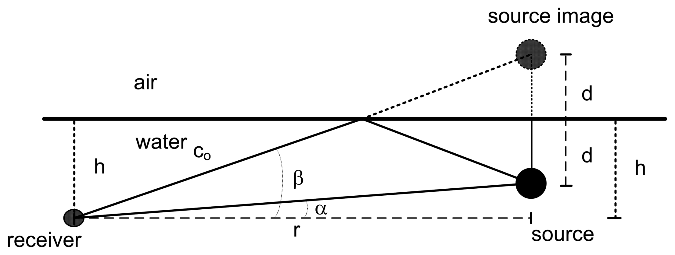
Assuming that the sound speed profile is (approximately) isovelocity and that the geometry of the experiment allows for a direct and a surface-reflected echo between the source and the receiver, the source range and depth can be estimated by simple geometric relations based on the source image method (Figure 1). α being the elevation of the direct echo and β the elevation of the surface-reflected echo as seen by the receiver, the source range, r, and depth, d, are related by the following equations:
3. Numerical Examples
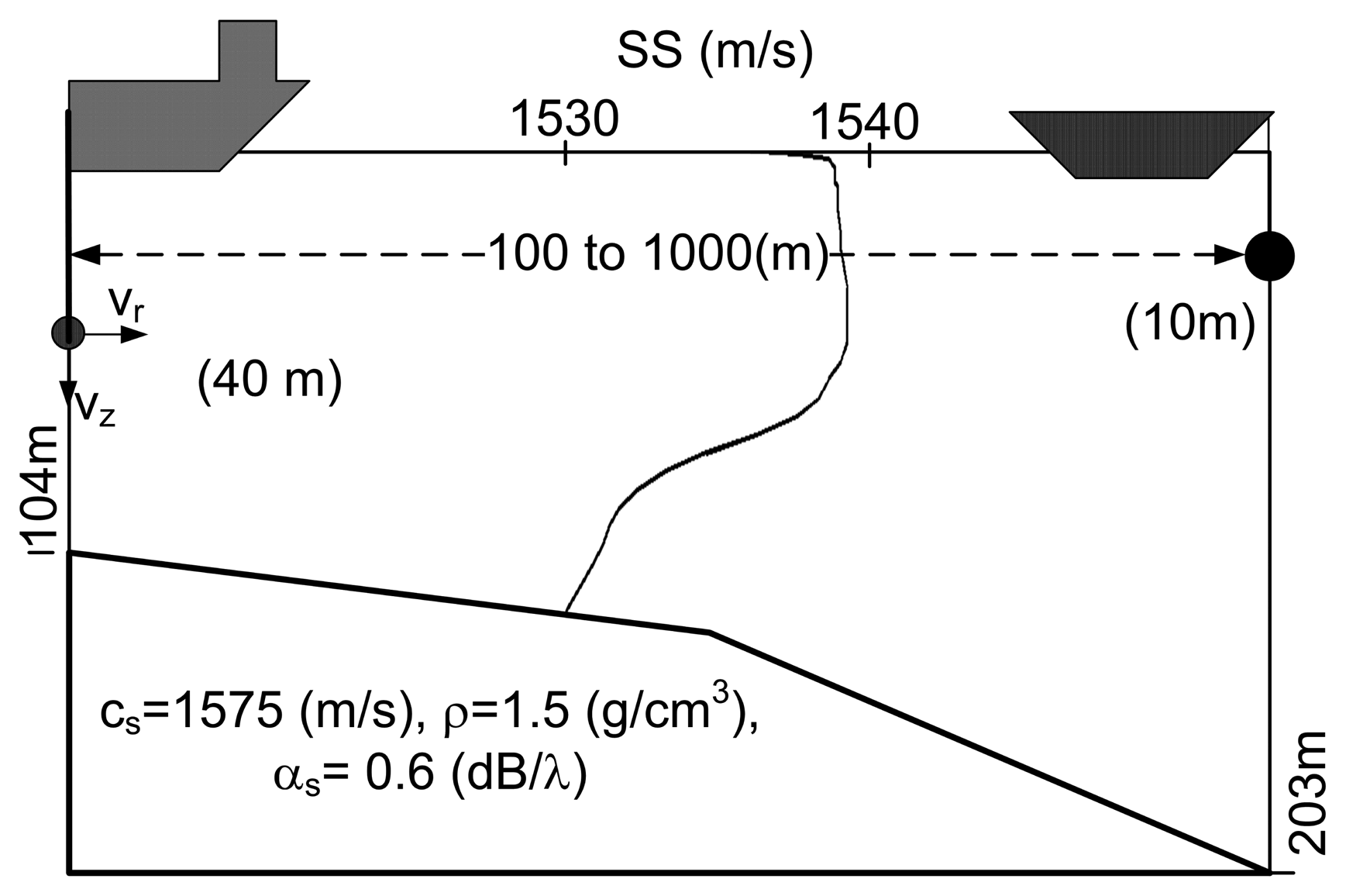
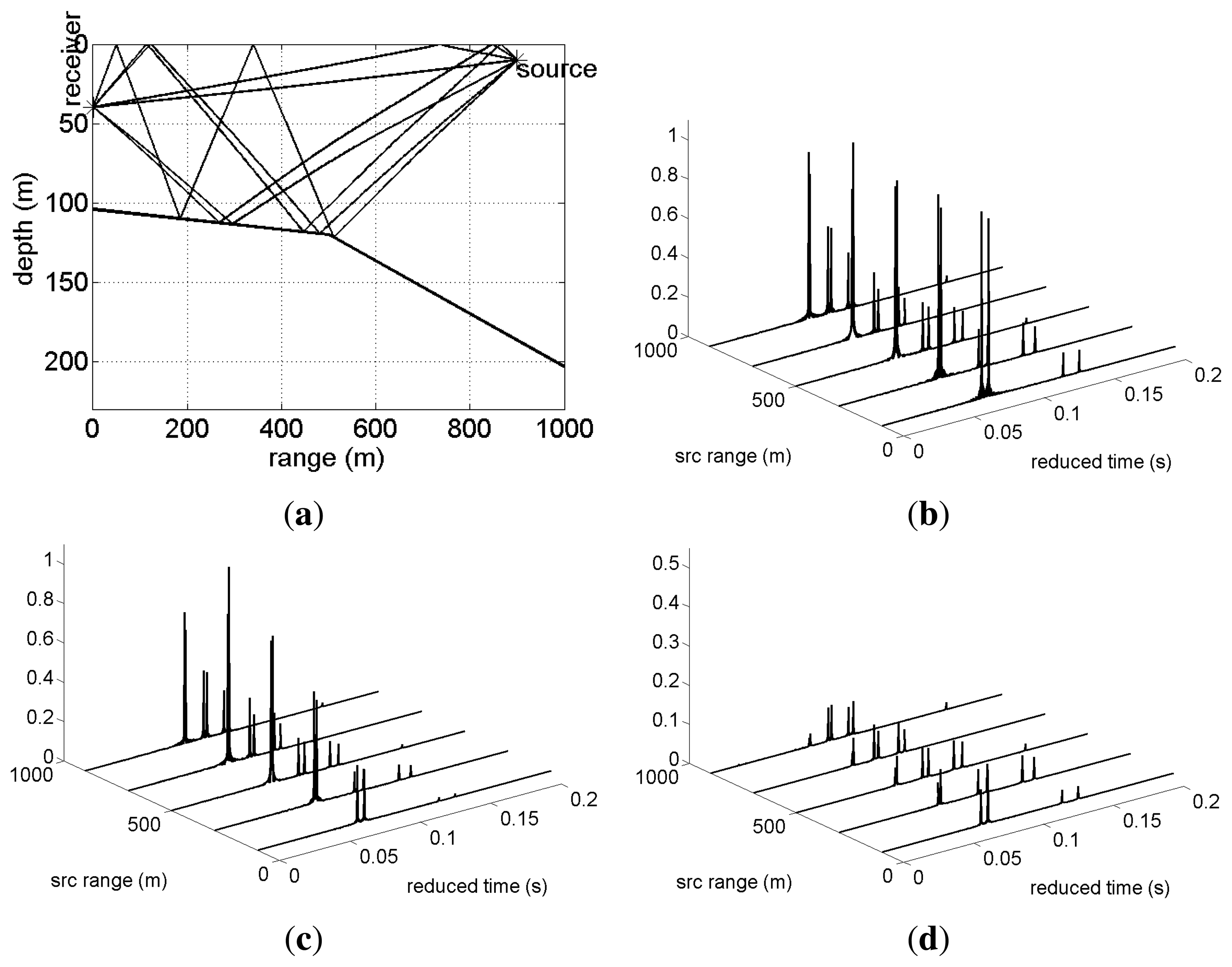
For testing the methods presented in the previous section and anticipating their performance on real data, the environmental and geometry scenario used for simulation is based on that of the Makai Experiment [34]. The simulation scenario is shown in Figure 2, where a vector sensor is suspended from a research vessel at 40 m depth. The sound source was suspended at 10 m depth and moved along a straight line between 100 m and 1,000 m range from the receiver, transmitting a linear frequency-modulated (LFM) chirp with a duration of 50 ms and a frequency band of 8–14 kHz. The bathymetry is range-dependent with water depth 104 m at the receiver and 203 m at the source when at 1,000 m range. The sound speed profile at the vector sensor location is represented in Figure 2, showing a thick mixed layer with a thermocline starting at 60 m depth. The bottom was modeled as a half-space characterized by the values estimated in [10]: a bottom compressional speed of 1,575 m/s, a density of 1.5 g/cm3 and a compressional attenuation of 0.6 dB/λ. In these simulations, it will be assumed that the azimuth is known; thus, only horizontal and vertical particle velocity components are considered. The channel pressure and particle velocity field frequency response were modeled by the cTraceo ray tracing model [35]. The time domain received waveforms were computed by Fourier synthesis. Figure 3 shows the eigenrays (paths of the echoes that impinge on the receiver) when the source is at a range of 900 m (Figure 3(a)) and the arrival patterns for the pressure, horizontal and vertical particle velocity (Figure 3(b–d), respectively). The arrival patterns for the pressure are normalized by the overall maximum, whereas the arrival patterns for the particle velocity components are normalized by the joint overall maximum. Note that the scale used for the particle velocity arrival patterns are different. In the eigenrays plot, one can notice a direct echo and a surface reflected echo, which correspond to the earliest peaks in the arrival patterns plots. These echoes have low angles relative to the horizontal plane containing the source, which decrease with an increasing source-receiver range. This behavior is observed in the particle velocity components, especially in the vertical component, where the amplitude of the peaks in the first cluster decreases as the source gets further way from the receiver. The latter echoes are bottom reflected. These echoes are also clustered in groups of two echoes depending on the number of surface reflections. Bottom reflected echoes have wider angles and lower amplitudes (especially pressure), mainly due to the attenuation in the bottom. Note that in the vertical particle velocity arrival patterns, the latter peaks have relatively higher amplitudes, since for wider angles, the module of sin(Φ) tends to unity. The amplitudes of the different echoes as seen by the vector sensor components illustrate, in the time domain, the spatial filtering capabilities of a single vector sensor.
A number of 100 realizations were generated according to model Equation (8), but limited to a horizontal and a vertical vector sensor component and source ranges from 100 to 900 m. The additive noise was independent for each component and obeyed a Gaussian distribution. Two different signal to noise ratios (SNR), 5 and 20 dB, at the receiver were generated. Since, in the considered geometry, the received energy in the horizontal component is higher than in the vertical component, as can be seen from the arrival structure shown in Figure 3, the SNR is related to the horizontal component, thus representing the worst case scenario. The elevation angles of the four earlier echoes impinging on the vector sensor were estimated independently for the different realizations. Then, the mean and the standard deviation were computed for each echo from the realization ensemble. In order to reduce time and amplitude discretization-related errors, the sampling frequency of the received waveforms (48 kHz) was increased (interpolated) by a factor of 10. The results are summarized in Table 1, where the lines labeled true show the values predicted by the forward ray tracing model.
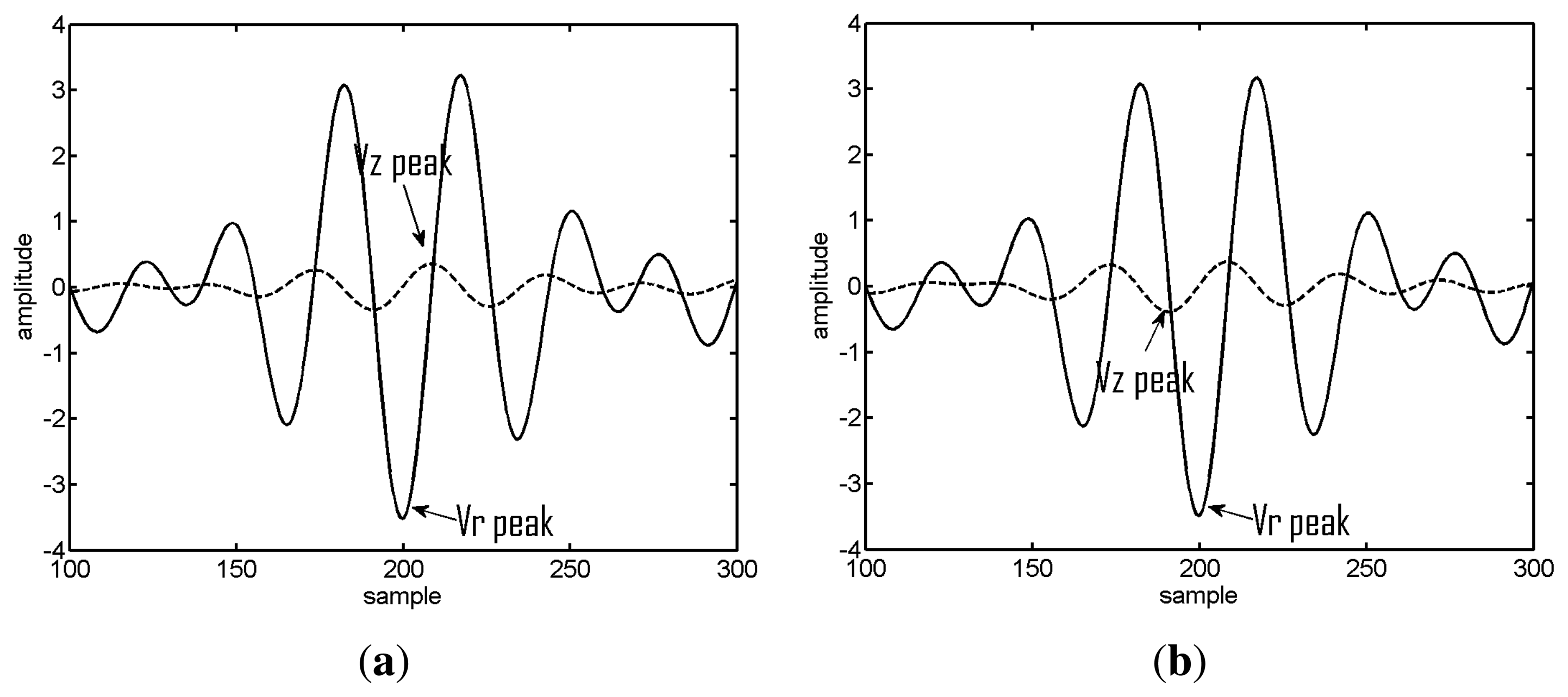
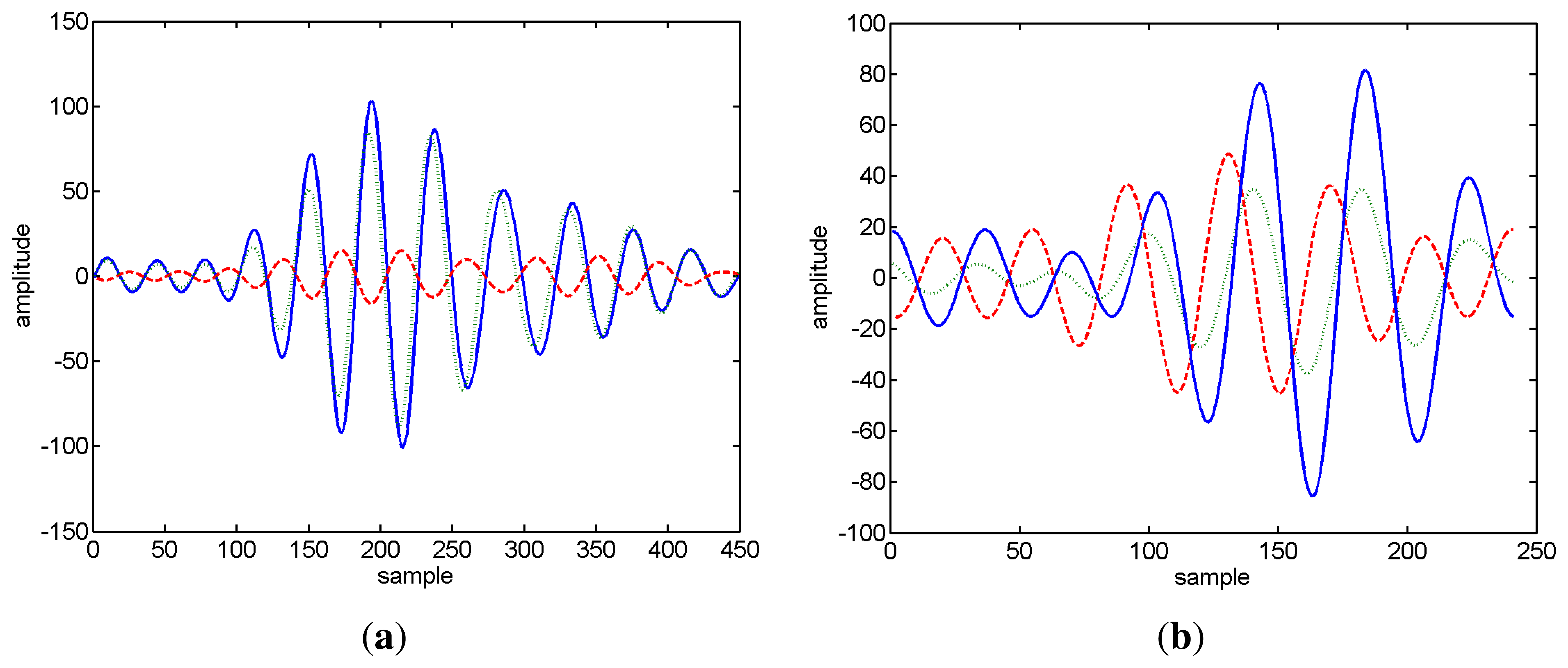
The values in brackets represent the standard deviation. The star mark appears when a sign error occurs at least once in the ensemble of realizations for the given echo. It can be seen that the absolute errors are always smaller then 1.2 degrees, and as expected, the standard deviation increases with decreasing SNR. Generally, the SNR at the receiver for distant signals decreases, which, in turn, also contributes to a higher variance of the estimates. Unsurprisingly, the sign error of the estimates increases significantly with decreasing SNR. The autocorrelation function of an LFM chirp is an oscillatory function; thus, due to the noise, the location of the absolute maximum that determines the sign of the elevation estimates can be shifted by an oscillation period, therefore resulting in a sign error. This situation is illustrated in Figure 4, showing the amplitude-delay curve (horizontal and vertical particle velocity) in the neighborhood of the first echo for two realizations at a source range of 300 m. One can observe that the sign of the peak of the vertical particle velocity changed among realizations. This sign ambiguity of the elevation estimates could be, in principle, minimized using a second vector sensor.
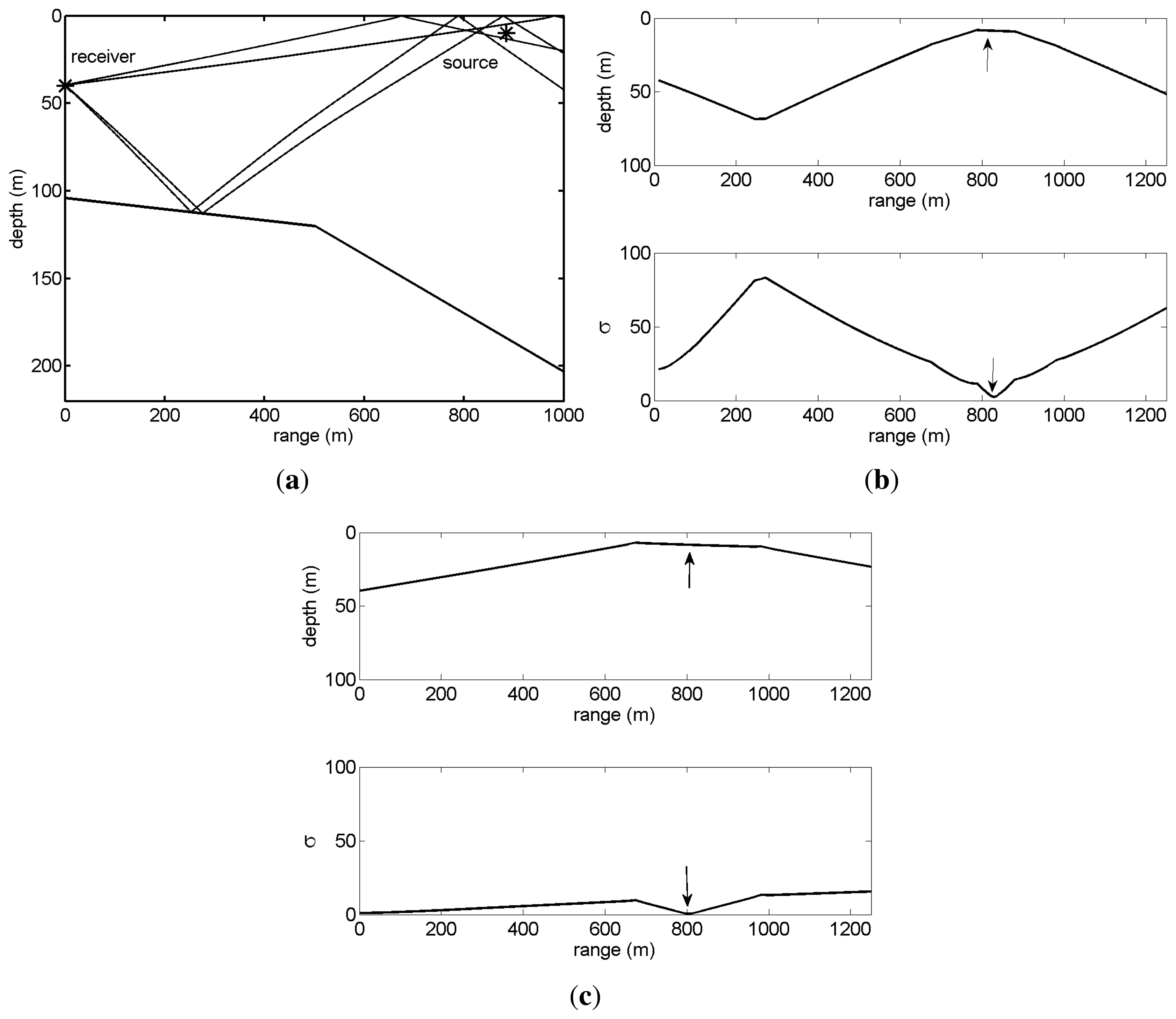
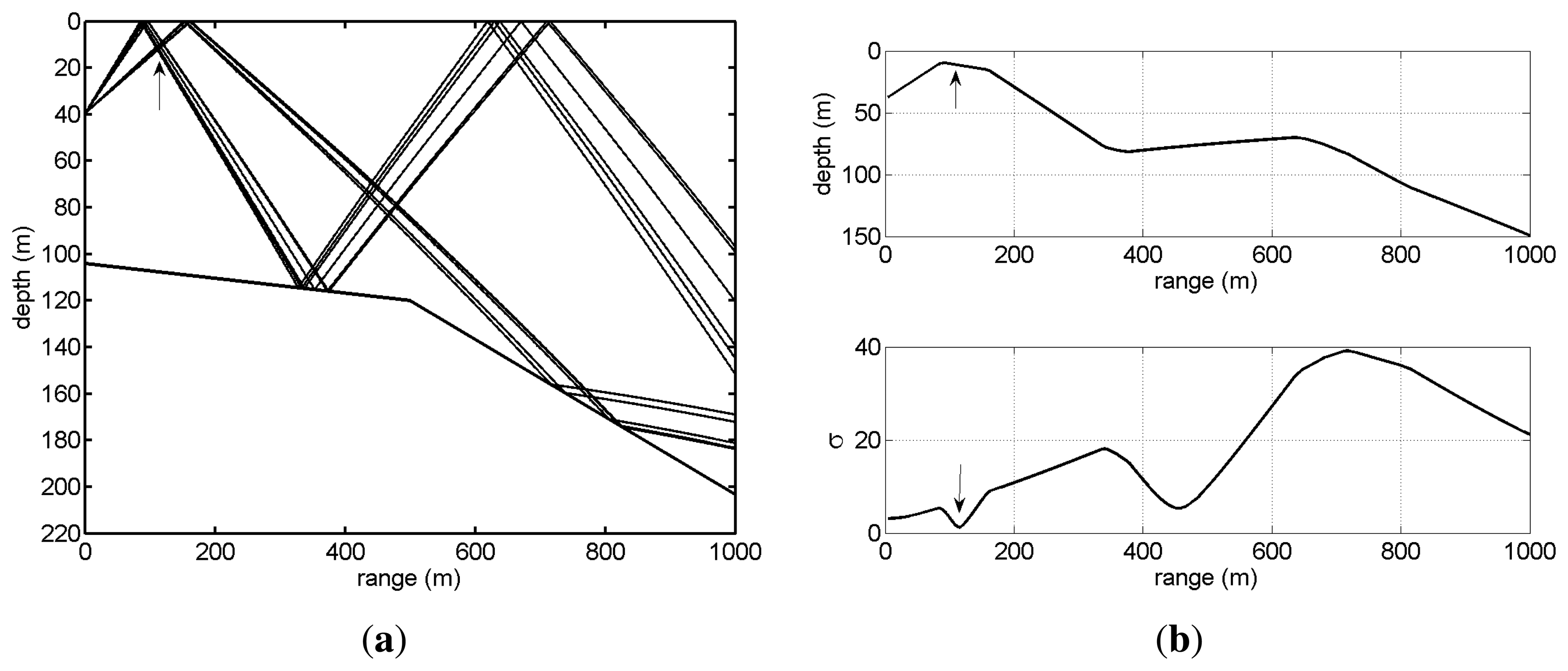
Next, using the elevation angle estimates for the 5 dB SNR presented in Table 1 and respective arrival times (not shown), the source range and depth were estimated applying the ray backpropagation and source-image method. For the ray backpropagation method, the estimates were obtained considering three different sets of echoes (the results are summarized in Table 2): all four echoes, the direct and the surface reflected echoes only (column labeled echoes 1&2) and the bottom reflected echoes only (column labeled echoes 3& 4). For the image method only, the direct and surface-reflected echoes are considered. Figure 5 illustrates the backpropagation method when the source is at a 900 m range. Figure 5(a) presents the backpropagated rays, where one can notice that the rays do not intercept at a single point, due to angle and travel time estimation errors. The objective function dependence in the range is plotted for four echoes in Figure 5(b) and for two echoes in Figure 5(c). For each case, the estimated source range is given by the minimum of the objective function and corresponding depth (respectively, lower and upper plots of Figure 5(b,c)). Whereas the objective function for four backpropagated rays has a single sharp minimum (Figure 5(b)) when only two rays are backpropagated, the shape of the objective function is smooth, giving rise to an increased ambiguity (Figure 5(c)), especially in ranges close to the receiver, because of the very short relative time delay between echoes and the close shooting angles.
Generally, range and depth estimation errors increase with source range, since small angle perturbations from the nominal value give rise to larger range depth perturbations. However, the errors are less than 2 m in depth and 75 m in range at the maximum range of 900 m, the worst case considered. The results obtained from the latter echoes, which are bottom reflected, present higher estimation errors than those obtained from direct and surface reflected echoes. Bottom reflection is frequency dependent, which is accounted for by the forward propagation model used to synthesize the received signal; however, the backpropagation uses only the echo path and travel time computed at a given frequency (in general, the middle frequency of the signal band). Moreover, bottom reflected echoes are more attenuated (depending on the bottom structure and the angle of incidence); thus, they are more affected by noise. One can also notice that the source image method gives reasonable estimates in the considered scenario, even at longer ranges, because the sound speed profile is almost isovelocity in the source-receiver layer.
4. Experimental Data Results
4.1. Experimental Setup
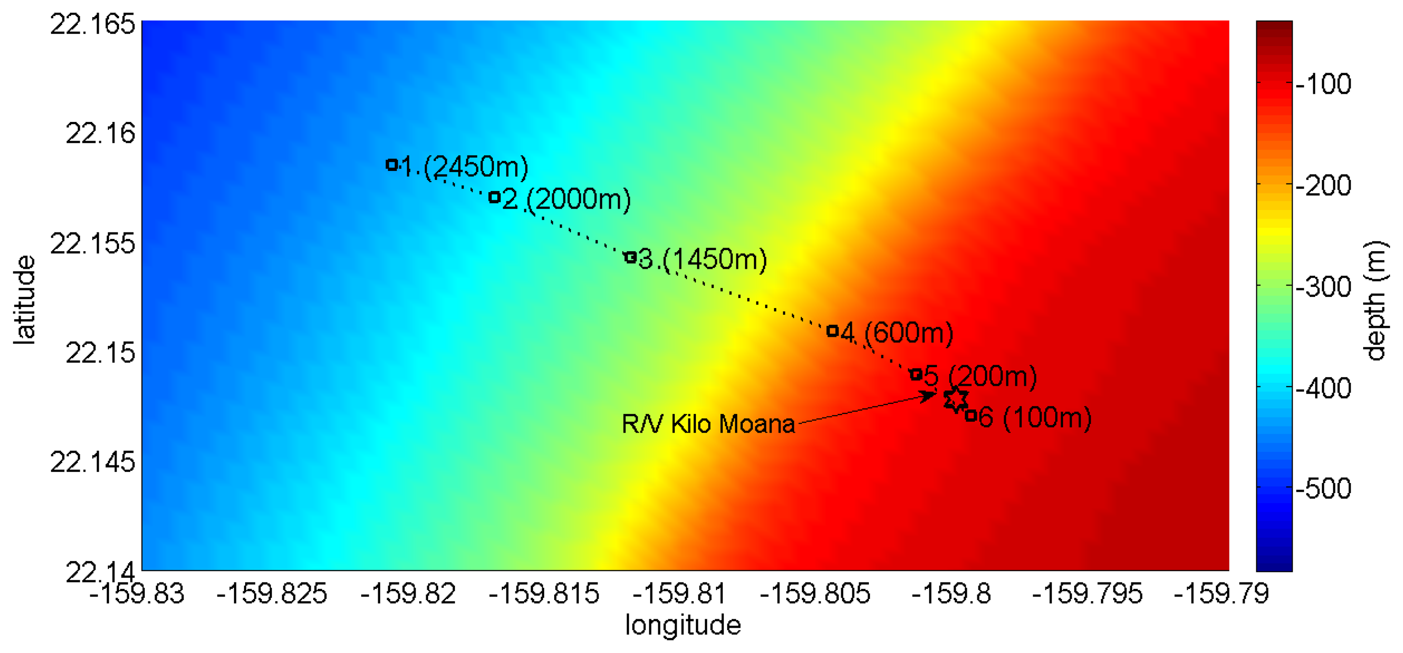
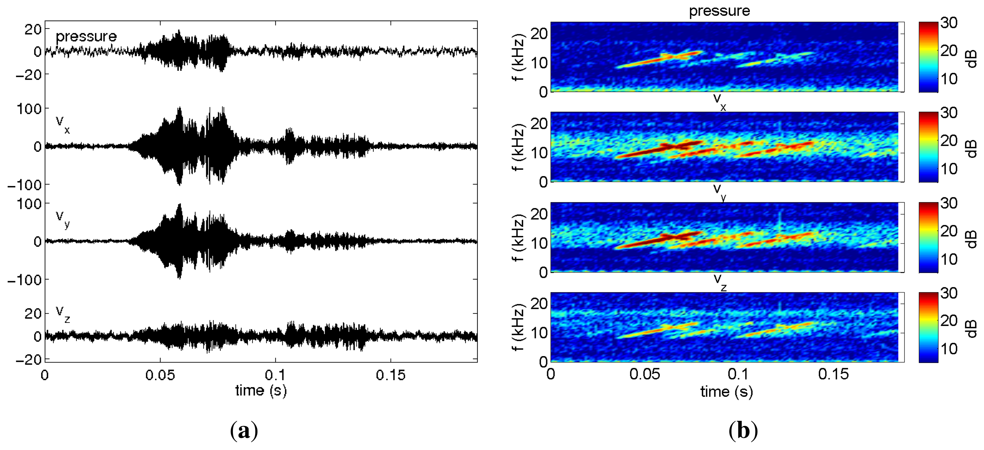
The data set analyzed here was acquired during the Makai Experiment (Makai'05), which took place off the west coast of Kauai I. in September 2005. The Makai'05 experiment was devoted to high frequency acoustics, and details of the experimental setup are described in [34]. This paper is concerned with the data acquired during the field calibration event, whose geometry is identical to that used in the numerical example (Figure 2). The vector sensor acquisition system used in the experiment was composed by four Wilcoxon TV-001 vector sensors [1,6,22], configured in a vertical array with 10 cm element spacing. The system was suspended off the stern of the research vessel, Kilo Moana, with a 150 kg weight at the bottom, to ensure that the array stayed as close to the vertical as possible. The z-axis was vertically oriented downwards, with the deeper sensor at 40 m. In the present data analysis, only the vector sensor at 40 m is considered. In the field calibration event, a Lubell 916C sound source deployed at 10 m depth from a small rubber boat was towed during a period of one hour from a 2.5 km distant point towards the research vessel that was holding a fixed position. Figure 6 shows the rubber boat GPS fixes and the research vessel (R/V) Kilo Moana location superimposed on the bathymetry of the area. The rubber boat track starts at a deeper location, moving along the continental steep slope towards a smooth and uniform area with a water depth of approximately 104 m. The source signals used for localization in this work were transmitted at various locations between approximately 600 m northwest and 100 m southeast of the R/V Kilo Moana, respectively, GPS fixes 4 and 6 in Figure 6. Ground truth measurements were carried out in this area during previous experiments and showed that most of the bottom in the area is covered with coral sands over a basalt hard bottom. The acoustic parameters of the sediment were estimated by Santos et al. [10], for the bottom compressional speed, attenuation and density—values already used in Section 3 of this paper. The Lubell 916C sound source transmitted 50 ms long LFM chirps spanning the 8–14 kHz band, transmitted in blocks of 30 chirps from various ranges along the track. The signals were acquired at a sampling frequency of 48 kHz. Due to a technical problem, the time stamp in the data is not synchronized with GPS; therefore, the precise position of the source for the various blocks of acquired data is not available. Figure 7 shows the time series (Figure 7(a)) and spectrograms (Figure 7(b)) of the received waveforms, when the source was at approximately 350 m range, where a strong multipath effect can be seen. The response of the vertical component should also be noted, which emphasizes the latter arrivals when compared with pressure or horizontal components: the relative amplitude of the latter arrival appearing approximately at 0.1 s is in the vertical component, higher than in the other components. This differentiating spatial response of the vertical component was explored in [10,36] to enhance the resolution of bottom parameter estimates. Technical problems with the gain of the pre-amplifiers explain why the amplitude of signals received from larger distances and those that suffer bottom reflections, which are more attenuated, is very low. In the next section, only the transmissions at a source-receiver range smaller than 500 m and the direct and surface reflected arrivals are considered.
4.2. Azimuth, Elevation and Travel Time Estimates
The received signal was filtered for a ship noise band (90–350 Hz) and an acoustic source band (8–14 kHz) by linear phase bandpass filtering. The ship noise was used to determine the orientation of the x-axis relative to the ship. For this purpose, the azimuth of the ship noise was estimated using the intensity-based method. The estimates were obtained by applying Equation (6) to ship noise received simultaneously with LFM chirps. The azimuth estimates are presented in a reference frame, where the x-axis is aligned west-east and the y-axis is aligned south-north. The elevation angles are considered positive towards the surface. The azimuth estimates obtained from the ship noise are very stable along the whole experiment [24,37].
As a first step to localize the source, the arrival times and amplitudes of the various echoes impinging on the vector sensor from each transmitted chirp were estimated from the arrival patterns using Equation (11). Since the transfer function of the transmission chain was unknown, a simulated undistorted LFM chirp was used in the amplitude arrival time estimation procedure. In order to increase the travel time and amplitude resolution, the acquired signal was up sampled by a factor of 10, becoming the virtual sampling frequency of 480 kHz. Figure 8 shows the delay-amplitude curve in the neighborhood of the first echo for the three vector sensor components at two different source ranges, illustrating that the travel time of an echo varies significantly among vector sensor components. While in Figure 8(a), the various components are nearly in phase, in Figure 8(b), a significant deviation occurs. Data inspection revealed that the perturbations varied among distances and among echoes, but were stable for the same echo number among transmissions at a given distance. Thus, for azimuth and elevation estimates, using Equations (12) and (13), respectively, the different components were treated independently. The amplitude of a given component was considered, where its absolute maximum occurs, whereas the associated travel time to be used in the backpropagation algorithm was that of the z-component. For the reasons explained above, only the direct and surface-reflected echoes were used for source range-depth estimation. For each distance, six chirps in the signal block were processed; azimuth and elevation were estimated. For the azimuth estimation only, the direct echo was considered. Table 3 presents the mean values and the standard deviations of those estimates, and for the sake of clarity, the range estimates are discussed in next section. As discussed in the numerical examples, the sign of the estimates suffer from a large ambiguity; thus, the sign of the elevation angle of the chirp echoes was assigned using the previous knowledge of the geometry. However, the sign of the azimuth of the ship noise was determined directly from the data. The orientation of the vector sensor relative to the R/V Kilo Moana given by the azimuth estimates from the ship noise was stable along time. This behavior was also observed for the other Makai'05 events for a full vector sensor array [37] and a single vector sensor [24]. One should note that the standard deviations of the elevation angles are lower for direct than for surface reflected echoes, which have a smaller amplitude and are subject to perturbations induced by the ocean surface. The high standard deviation of azimuth estimates at position min 54 and min 57 can be explained by the shorter range. A horizontal displacement at a shorter range gives rise to a higher azimuth perturbation when compared with similar displacement at a longer range.
4.3. Range-Depth Estimates
The range and depth of the source were estimated with the ray backpropagation method using the elevation angles of the direct and surface reflected echoes and respective relative arrival times. In order to obtain an estimate of the standard deviation of the estimates, the objective function is an average of the objective functions computed for each single realization of the transmitted chirp signal. Figure 9(a) shows the direct and surface reflected backpropagated rays with elevation angles estimated from six chirps transmitted at min 57, where the source was at a range of 114 m. The overall objective function (ambiguity curve) dependence in the range computed from these rays (and travel time estimates) is shown in the lower plot of Figure 9(b), whereas the estimated source range is given by the minimum of the objective function and the corresponding depth in the upper plot. The range and depth estimates at various source distances obtained by backpropagation are presented in Table 4. Column σ represents the minimum of the square root of the objective function, where the smaller values (smaller variance), are attained at closer ranges. Model-based source localization methods are, in general, not considered for real-time implementations, because of the time needed to compute the optimization procedure, which requires a large number of forward model runs, but a non-optimized Matlab implementation of the ray backpropagation method took less than 4 s in a current laptop. It is expected that further code optimization would allow for real-time application.
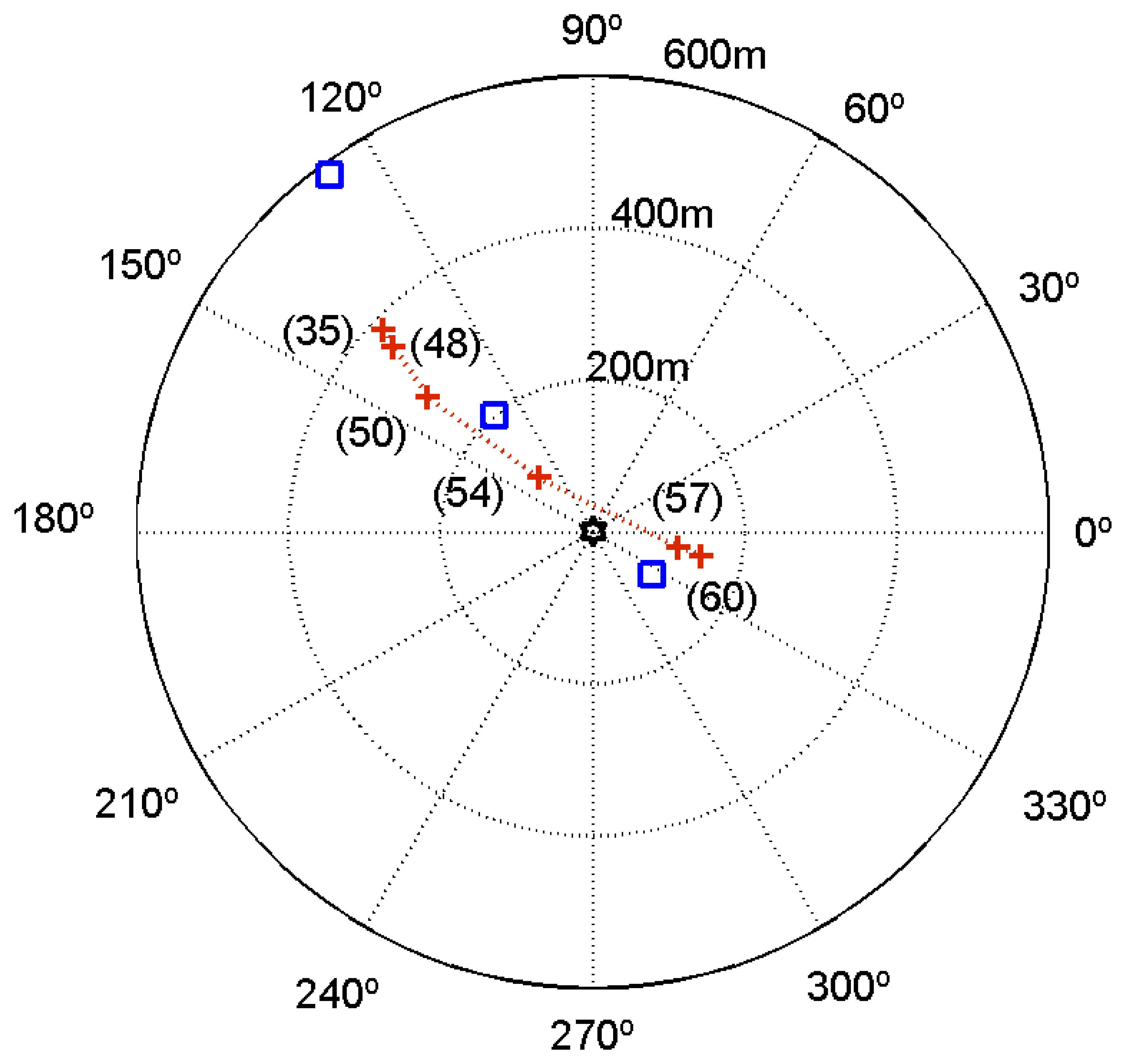
For comparison purposes the results obtained using the source image method are also shown in Table 4. At longer distances, the difference between the estimates obtained by both methods increases, due to the cumulative effect of considering a constant sound speed with the image method. One should remark that the source depth estimates are in close agreement with the nominal depth of the source of 10 m. Figure 10 shows a polar plot with the location of the source using the source range and azimuth estimates, which are represented by stars. The squares represent the positioning of the source relative to the R/V Kilo Moana (at the origin) estimated from the ship's GPS and a handheld GPS device on the source's boat. Unfortunately, the handheld GPS device had no recording capabilities; thus, the source path between GPS fixes is uncertain. Since the range estimates by GPS and by acoustics are affected by some offset, because of the different location of the vector sensor and GPS on board the R/V Kilo Moana, and there is no time stamp in the acoustic data, this did not allow for synchronization between acoustic and GPS data. The source track derived from acoustic data are in relatively close agreement with GPS fixes.
5. Conclusions
This paper illustrates the spatial filtering capabilities of a vector sensor applied to source localization of a known broadband signal in a multipath environment. It was shown that the estimation of the angle of arrival (elevation) of a single echo was possible. Given the estimates of the amplitudes of the echoes in the vx,vy and vz vector sensor components, a method to estimate the source azimuth and the elevation was presented. The elevation angles of the direct and surface reflected echoes were used to estimate source range and depth localization by a ray backpropagation algorithm. The method was discussed in the context of simulated data and for a real data set acquired during the Makai Experiment. It was shown that for ranges below 500 m, it was possible to estimate the source range and depth in agreement with the known geometry of the experiment. To the best of our knowledge, this is the first work in open literature that reports 3D localization results with a single vector sensor in a shallow water environment. In comparison with other model-based methods discussed in the literature for source localization using a single device (hydrophone), the present method explores the spatial filtering capabilities of a single vector sensor to significantly reduce the number of forward model runs; thus, it can be potentially implemented in low end or light real-time systems.
Acknowledgments
The authors would like to thank Michael Porter, chief scientist for the Makai Experiment, Jerry Tarasek for the loan of the vector sensor array used in the experiment and Paul Hursky, Martin Siderius and Bruce Abraham for providing assistance with the data acquisition. The Makai Experiment was supported by the US Office of Naval Research. This work was funded by National Funds through Foundation for Science and Technology (FCT) under project SENSOCEAN (PTDC/EEA-ELC/104561/2008).
Conflict of Interest
The authors declare no conflict of interest.
References
- Silvia, M.T.; Richards, R.T. A Theoretical and Experimental Investigation of Low-frequency Acoustic Vector Sensors. Proceedings of the Oceans 2002 Conference (OCEANS'02), Biloxi, MI, USA, 29–31 October 2002.
- D'Spain, G.; Hogkiss, W.S.; Edmonds, G.L. Initial Analysis of the Data from the Vertical DIFAR Array. Proceedings of the Oceans 1992 Conference (OCEANS'92), Newport, USA, 26–29 October 1992.
- Miron, S.; Le Bihan, N.; Mars, J.I. Vector-sensor MUSIC for polarized seismic sources localization. J. Appl. Signal Process. 2005, 2005, 74–84. [Google Scholar]
- Miron, S.; Le Bihan, N.; Mars, J. Quaternion-MUSIC for vector-sensor array processing. Signal Process. IEEE Trans. 2006, 54, 1218–1229. [Google Scholar]
- Tam, P.K.; Wong, K.T. Cramér-Rao bounds for direction finding by an acoustic vector sensor under nonideal gain-phase responses, noncollocation, or nonorthogonal orientation. IEEE Sens. J. 2009, 9, 969–982. [Google Scholar]
- Shipps, J.C.; Abraham, B.M. The Use of Vector Sensors for Underwater Port and Waterway Security. Proceedings of the ISA/IEEE Sensors for Industry Conference, New Orleans, LA, USA, 24 August 2004.
- Song, A.; Badiey, M.; Hursky, P.; Abdi, A. Time Reversal Receivers for Underwater Acoustic Communication Using Vector Sensors. Proceedings of the Oceans 2008 Conference (OCEANS'08), Quebec City, Canada, 15–18 September 2008.
- Han-Shu, P.; Feng-Hua, L. Geoacoustic inversion based on a vector hydrophone array. Chin. Phys. Lett. 2007, 24, 1977–1980. [Google Scholar]
- Santos, P.; Rodriguez, O.; Felisberto, P.; Jesus, S. Geoacoustic Matched-Field Inversion Using a Vertical Vector Sensor Array. Proceedings of the 3rd International Conference and Exhibition on Underwater Acoustic Measurements: Technologies and Results, Nafplion, Greece, 21–26 June 2009; pp. 29–34.
- Santos, P.; Rodriguez, O.C.; Felisberto, P.; Jesus, S.M. Seabed geoacoustic characterization with a vector sensor array. J. Acoust. Soc. Am. 2010, 128, 2652–2663. [Google Scholar]
- Miron, S.; Le Bihan, N.; Mars, J. Joint Estimation of Direction of Arrival and Polarization Parameters for Multicomponent Sensor Array. Proceedings of the 66th European Association of Geoscientists and Engineers Conference and Exhibition, Paris, France, 7–10 June 2004.
- Sherman, C.H.; Butler, J.L. Transducers and Arrays for Underwater Sound; The Underwater Acoustic series, Springer: Berlin/Heidelberg, Germany, 2007. [Google Scholar]
- Wu, Y.I.; Wong, K.T.; Yuan, X.; Lau, S.K.; keung Tang, S. A directionally tunable but frequency-invariant beamformer on an acoustic velocity-sensor triad to enhance speech perception. J. Acoust. Soc. Am. 2012, 131, 3891–3902. [Google Scholar]
- Liu, X.; Xiang, J.; Zhou, Y. Passive tracking and size estimation of volume target based on acoustic vector intensity. Chin. J. Acoust. 2001, 20, 225–238. [Google Scholar]
- Awad, M.; Wong, K. Recursive least-squares source tracking using one acoustic vector sensor. Aerosp. Electron. Syst. IEEE Trans. 2012, 48, 3073–3083. [Google Scholar]
- Rahamim, D.; Tabrikian, J.; Shavit, R. Source localization using vector sensor array in a multipath environment. Signal Process. IEEE Trans. 2004, 52, 3096–3103. [Google Scholar]
- Arunkumar, K.; Anand, G. Source Localisation in Shallow Ocean Using Vertical Array of Acoustic Vector Sensors. Proceedings of the European Signal Processing Conference (EUSIPCO), Poznan, Poland, 3–7 September 2007; pp. 2454–2458.
- Hurtado, M.; Nehorai, A. Performance analysis of passive low-grazing-angle source localization in maritime environments using vector sensors. Aerosp. Electron. Syst. IEEE Trans. 2007, 43, 780–789. [Google Scholar]
- Abdi, A.; Guo, H.; Sutthiwan, P. A New Vector Sensor Receiver for Underwater Acoustic Communications. Proceedings of the Oceans 2007 Conference (OCEANS'07), Vancouver, Canada, 29 September–4 October 2007.
- Hawkes, M.; Nehorai, A. Wideband source localization using a distributed acoustic vector-sensor array. IEEE Trans. Signal Process. 2002, 27, 628–637. [Google Scholar]
- Voltz, P.; Lu, I.T. A time-domain backpropagating ray technique for source localization. J. Acoust. Soc. Am. 1994, 95, 805–812. [Google Scholar]
- Abraham, B.M. Ambient Noise Measurements with Vector Acoustic Hydrophones. Proceedings of the Oceans 2006 Conference (OCEANS'06), Boston, MA, USA, 18–21 September 2006.
- Nehorai, A.; Paldi, E. Acoustic vector-sensor array processing. IEEE Trans. Signal Process. 1994, 42, 2481–2491. [Google Scholar]
- Felisberto, P.; Santos, P.; Jesus, S. Tracking Source Azimuth Using a Single Vector Sensor. Proceedings of the Fourth International Conference on Sensor Technologies and Applications (SENSORCOMM), Venice, Italy, 18–25 July 2010; pp. 416–421.
- Hermand, J.P. Broad-band inversion in shallow water from waveguide impulse response measurements on a single hydrophone: Theory and experimental results. IEEE J. Ocean. Eng. 1999, 24, 41–66. [Google Scholar]
- Jesus, S.; Porter, M.; Stéphan, Y.; Démoulin, X.; Rodriguez, O.; Coelho, E. Single hydrophone source localization. IEEE J. Ocean. Eng. 2000, 25, 337–346. [Google Scholar]
- Gac, J.C.L.; Asch, M.; Stéphan, Y.; Démoulin, X. Geoacoustic inversion of broadband acoustic data in shallow water on a single hydrophone. IEEE J. Ocean. Eng. 2003, 28, 479–493. [Google Scholar]
- Felisberto, P.; Jesus, S.M.; Stephan, Y.; Demoulin, X. Shallow Water Tomography with a Sparse Array during the INTIMATE'98 Sea Trial. Proceedings of the MTS/IEEE Oceans 2003 Conference (OCEANS'03), San Diego, USA, 22–26 September 2003; pp. 571–575.
- Felisberto, P.; Rodriguez, O.; Jesus, S.M. Estimating the Multipath Structure of an Underwater Channel Using a Single Vector Sensor. Proceedings of the ECUA 2012 11th European Conference on Underwater Acoustics, Edinburgh, Scotland, 2–6 July 2013; Volume 17, pp. 1–9.
- Hawkes, M.; Nehorai, A. Acoustic vector-sensor correlations in ambient noise. IEEE J. Ocean. Eng. 2001, 26, 337–347. [Google Scholar]
- Abdi, A.; Guo, H. Signal correlation modeling in acoustic vector sensor arrays. IEEE Trans. Signal Process. 2009, 57, 892–903. [Google Scholar]
- Wu, Y.; Wong, K.; Lau, S.K. The acoustic vector-sensor's near-field array-manifold. IEEE Trans. Signal Process. 2010, 58, 3946–3951. [Google Scholar]
- Meyer, M.; Hermand, J.P. Backpropagation Techniques in Ocean Acoustic Inversion: Time Reversal, Retrogation and Adjoint Modelling. In Acoustic Sensing Techniques for the Shallow Water Environment; Caiti, A., Chapman, N., Hermand, J.P., Jesus, S.M., Eds.; Springer: Dordrecht, The Netherlands, 2006; pp. 29–46. [Google Scholar]
- Porter, M.; Abraham, B.; Badiey, M.; Buckingham, M.; Folegot, T.; Hursky, P.; Jesus, S.; Kim, K.; Kraft, B.; McDonald, V.; et al. The Makai experiment: High frequency acoustics. Proceedings of the 8th ECUA European Conferece on Underwater Acoustic, Carvoeiro, Portugal, 12–15 June 2006; Volume 1, pp. 9–18.
- Rodriguez, O.; Collis, J.; Simpson, H.; Ey, E.; Schneiderwind, J.; Felisberto, P. Seismo-acoustic ray model benchmarking against experimental tank data. J. Acoust. Soc. Am. 2012, 132, 709–717. [Google Scholar]
- Felisberto, P.; Rodriguez, O.; Santos, P.; Jesus, S.M. On the Usage of the Particle Velocity Field for Bottom Characterization. Proceedings of the International Conference on Underwater Acoustic Measurements, Kos, Greece, 19–24 June 2011; pp. 19–24.
- Santos, P.; Felisberto, P.; Hursky, P. Source Localization with Vector Sensor Array during the Makai Experiment. Proceedings of the 2rd International Conference and Exhibition on Underwater Acoustic Measurements: Technologies and Results, Heraklion, Greece, 25–29 June 2007; pp. 895–900.


| Source Depth 10 m | Echo Number | |||||
|---|---|---|---|---|---|---|
| Range [m] | SNR [dB] | 1 [°] | 2 [°] | 3 [°] | 4 [°] | |
| 100 | True | 16.3 | 26.1 | −60 | −63 | model |
| 20 | 17.3 (0.1) | 27.3 (0.1) | −59.4 (0.5) | −62.5 (0.7) | estimate | |
| 5 | 17.3 (0.4) | 27.4 (0.4) | −59.4 (3.4) * | −62.1 (3.7) * | estimate | |
| 300 | True | 5.6 | 9.3 | −30.8 | −33.8 | model |
| 20 | 5.9 (0.1) | 9.9 (0.1) | −31.8 (0.4) | −34.4 (0.3) | estimate | |
| 5 | 5.9 (0.4) * | 10.1 (0.5) | −31.9 (2.3) * | −34.5 (2.0) * | estimate | |
| 500 | True | 3.3 | 5.5 | −20.7 | −22.8 | model |
| 20 | 3.7 (0.1) | 5.8 (0.1) | −21.8 (0.3) | −23.8 (0.3) | estimate | |
| 5 | 3.7 (0.5) * | 5.8 (0.5) | −21.9 (1.5) * | −24.0 (2.1) * | estimate | |
| 700 | True | 2.3 | 3.9 | −15.9 | −17.6 | model |
| 20 | 2.5 (0.1) | 4.1 (0.1) | −16.8 (0.2) | −18.8 (0.4) | estimate | |
| 5 | 2.7 (0.6) * | 4.1 (0.4) * | −16.8 (1.3) * | −18.7 (2.0) * | estimate | |
| 900 | True | 1.8 | 2.9 | −13.2 | −14.5 | model |
| 20 | 1.9 (0.1) | 3.1 (0.1) | −14.1(0.2) | −15.2 (0.2) | estimate | |
| 5 | 2.1 (0.5) * | 3.2 (0.5) * | −14.1 (1.0) * | −15.3 (1.0) * | estimate | |
| Simulated | Ray Backpropagation | Image Method | ||||||
|---|---|---|---|---|---|---|---|---|
| Depth 10 m | 4 Echoes | Echoes 1&2 | Echoes 3 &4 | Echoes 1&2 | ||||
| Range [m] | Range [m] | Depth [m] | Range [m] | Depth [m] | Range [m] | Depth [m] | Range [m] | Depth [m] |
| 100 | 102.5 | 10.0 | 99.4 | 10.2 | 104.3 | 9.7 | 95.7 | 9.9 |
| 300 | 299.3 | 10.2 | 300.1 | 11.3 | 290.3 | 8.9 | 282.1 | 10.5 |
| 500 | 499.4 | 9.8 | 500.9 | 9.5 | 469.1 | 9.4 | 477.6 | 8.8 |
| 700 | 649.1 | 9.6 | 668.1 | 8.2 | 640.2 | 8.3 | 649.5 | 10.9 |
| 900 | 829.2 | 8.6 | 804.5 | 8.4 | 830.1 | 8.4 | 857.7 | 8.3 |
| Time[min] | Source Range[m] | Azimuth[°] | Elevation[°] | ||
|---|---|---|---|---|---|
| Ship Noise 90–350 Hz | Source 8–14 kHz | Dir.Echo | Surf.Ref.Echo | ||
| 35 | 386.3 | 132.4 | 136.1 (0.2) | 4.1 (0.1) | 7.5 (0.1) |
| 48 | 357.5 | 132.2 | 137.3 (0.8) | 4.9 (0.1) | 7.5 (0.7) |
| 50 | 279.8 | 134.4 | 140.9 (0.4) | 5.5 (0.3) | 9.8 (1.3) |
| 54 | 100.8 | 133.1 | 135.1 (2.3) | 16.7 (0.2) | 25.7 (2.0) |
| 57 | 114.2 | 131.7 | −10.2 (1.0) | 14.0 (0.4) | 23.8 (1.0) |
| 60 | 145.4 | 132.2 | −12.6 (0.6) | 12.4 (0.2) | 17.8 (1.1) |
| Time [min] | Ray Backpropagation | Image Method | |||
|---|---|---|---|---|---|
| Range [m] | Depth [m] | σ [m] | Range [m] | Depth [m] | |
| 35 | 386.3 | 10.54 | 6.7 | 391.1 | 11.7 |
| 48 | 357.5 | 10.55 | 9.4 | 367.1 | 8.3 |
| 50 | 279.8 | 11.1 | 1.8 | 298.8 | 11.0 |
| 54 | 100.8 | 10.1 | 1.5 | 101.9 | 9.2 |
| 57 | 114.2 | 11.5 | 1.0 | 115.0 | 11.0 |
| 60 | 145.4 | 7.9 | 1.2 | 146.7 | 7.3 |
© 2013 by the authors; licensee MDPI, Basel, Switzerland. This article is an open access article distributed under the terms and conditions of the Creative Commons Attribution license (http://creativecommons.org/licenses/by/3.0/).
Share and Cite
Felisberto, P.; Rodriguez, O.; Santos, P.; Ey, E.; Jesus, S.M. Experimental Results of Underwater Cooperative Source Localization Using a Single Acoustic Vector Sensor. Sensors 2013, 13, 8856-8878. https://doi.org/10.3390/s130708856
Felisberto P, Rodriguez O, Santos P, Ey E, Jesus SM. Experimental Results of Underwater Cooperative Source Localization Using a Single Acoustic Vector Sensor. Sensors. 2013; 13(7):8856-8878. https://doi.org/10.3390/s130708856
Chicago/Turabian StyleFelisberto, Paulo, Orlando Rodriguez, Paulo Santos, Emanuel Ey, and Sérgio M. Jesus. 2013. "Experimental Results of Underwater Cooperative Source Localization Using a Single Acoustic Vector Sensor" Sensors 13, no. 7: 8856-8878. https://doi.org/10.3390/s130708856
APA StyleFelisberto, P., Rodriguez, O., Santos, P., Ey, E., & Jesus, S. M. (2013). Experimental Results of Underwater Cooperative Source Localization Using a Single Acoustic Vector Sensor. Sensors, 13(7), 8856-8878. https://doi.org/10.3390/s130708856