Error Modeling and Calibration for Encoded Sun Sensors

Abstract
: Error factors in the encoded sun sensor (ESS) are analyzed and simulated. Based on the analysis results, an ESS error compensation model containing structural errors and fine-code algorithm errors is established, and the corresponding calibration method for model parameters is proposed. As external parameters, installation deviation between ESS and calibration equipment are introduced to the ESS calibration model, so that the model parameters can be calibrated accurately. The experimental results show that within plus/minus 60 degree of incident angle, the ESS measurement accuracy after compensation is three times higher on average than that before compensation.1. Introduction
The encoded sun sensor (ESS), an important attitude measurement component in the satellite attitude control system [1,2], is at present successfully applied in ninety percent of Chinese satellites for its simple structure and proven technology. However, its accuracy is limited by manufacturing tolerances of the components, assembly deviations and algorithm approximation errors in signal processing, etc. If an effective model cannot be found to compensate these errors, the measurement accuracy of a traditional ESS will not meet the increased demands of the spacecraft [3], so in this paper, error factors which reduce the accuracy of encoded sun sensors are analyzed. Accordingly an error compensation model for an encoded sun sensor is established, and an accurate calibration method for model parameters is also proposed.
2. Structure and Working Principle of ESS
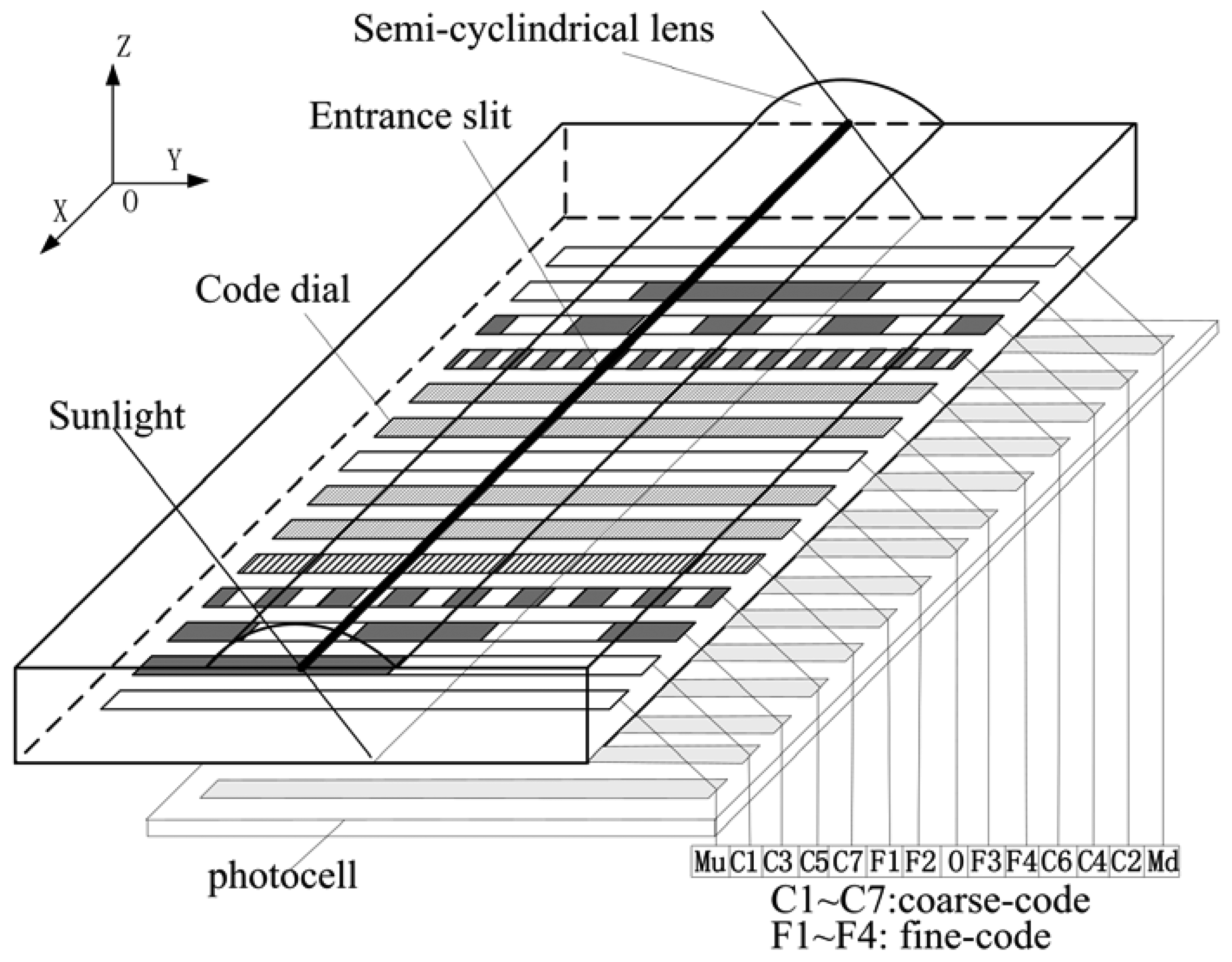
An encoded sun sensor is mainly made up of an optical sensing unit and signal processing circuits. The optical sensing unit usually includes optical components (such as a semi-cylindrical lens) with etched entrance slit, code dial and embedded photocell, as shown in Figure 1. Its working principle is: Sunlight is projected onto the code dial through entrance slit in different incident angles. There is a series of encoded rows on the code dial. Each row is etched with an opaque-transparent alternating grid. Photocells beneath each encoded row receive sunlight through the code dial and convert them into a current signal which is related with the incident angle of sunlight. These current signals are further processed by signal processing circuit into an angle output.
3. Error Analysis of ESS
Each step of the imaging and signal processing has been investigated to find the possible error factors [4–6]. Simulation for two types of product has been done to estimate the degree of influence of the various error factors.
3.1. Distance Deviation between Entrance Slit and Code Dial
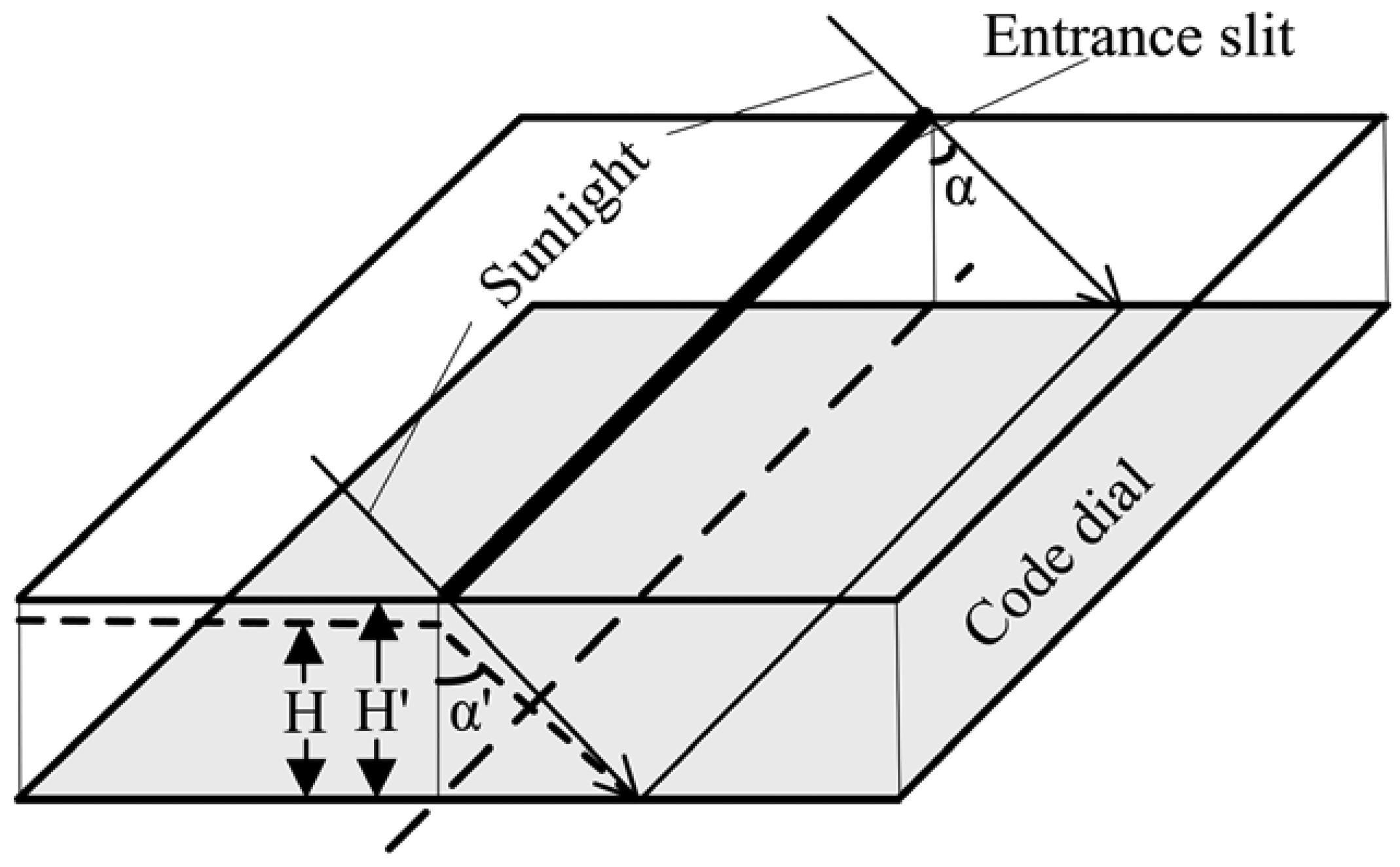
The encoded rows on code dial are etched according to the rule of y = H tan(α), where H is the distance between entrance slit and code dial. The ideal value of the distance is H, but there is always a deviation ΔH between ideal value and actual value due to limited manufacturing accuracy. Let y be the position of sunlight on the code dial when incident angle (i.e., measurement angle) is α. The output angle of ESS can be expressed as α′ = atan(y/H), while the actual incident angle of sunlight is α = atan(y/H′), which cause error as shown in Figure 2.
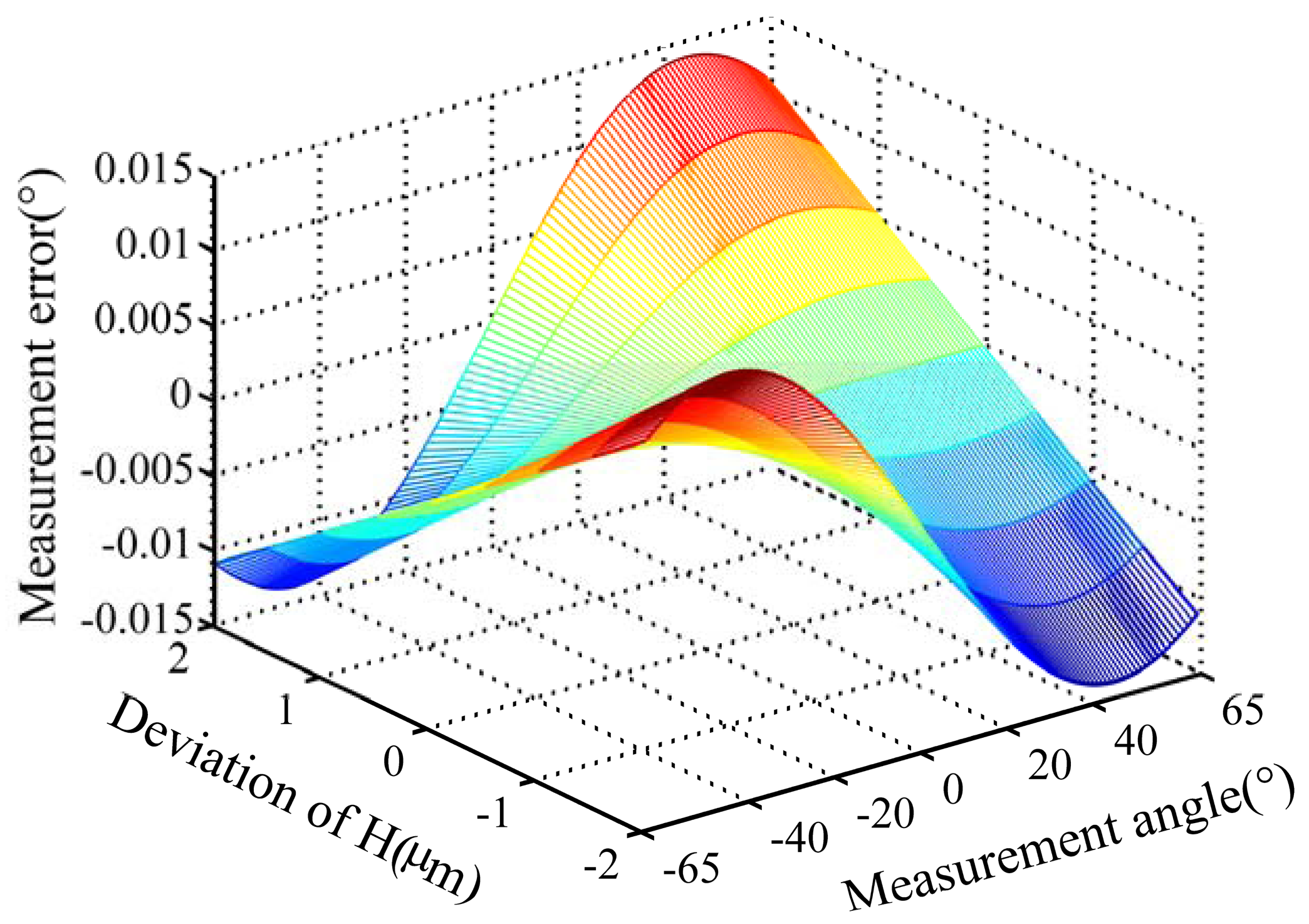
Measurement errors caused by distance deviation ΔH for two types of product (designated as A and B) were analyzed by simulation. The distance H is 4.124 mm for product A and 6.584 mm for product B. The simulation is done under the following conditione: distance deviation ΔH is ±2 microns, and the range of measurement angle is (−62°∼62°). Figure 3 shows the simulation result for product A.
Simulated results are as follows:
Measurement errors caused by distance deviation ΔH will increase when the distance between the entrance slit and code dial decreases or the incident angle increases.
For Product A, measurement error will exceed 0.015° when the distance deviation exceeds two micron, as shown in Figure 3. For Product B, measurement error will exceed 0.008° when the distance deviation exceeds two microns. It can be seen that the distance deviation ΔH will lead eventually to considerable measurement errors, so the distance deviation ΔH cannot be ignored.
3.2. Misalignment between Entrance Slit and Center Line of Code Dial
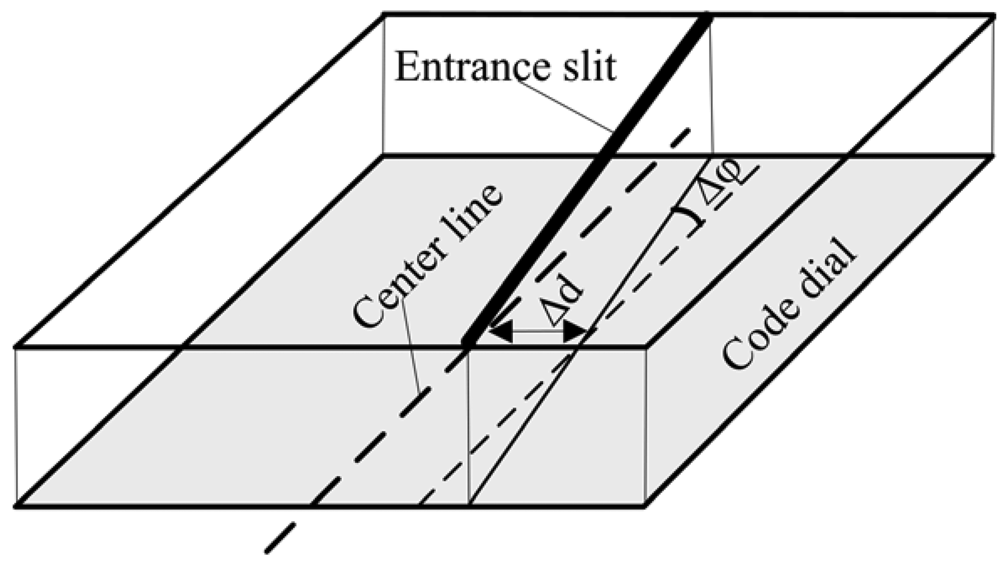
In an ideal condition, the entrance slit should be aligned with center line of the code dial, but due to assembly deviation between the semi-cylindrical lens and code dial, offset Δd and tilt Δφ between entrance slit and center line of code dial will inevitably occur, which cause errors as shown in Figure 4.
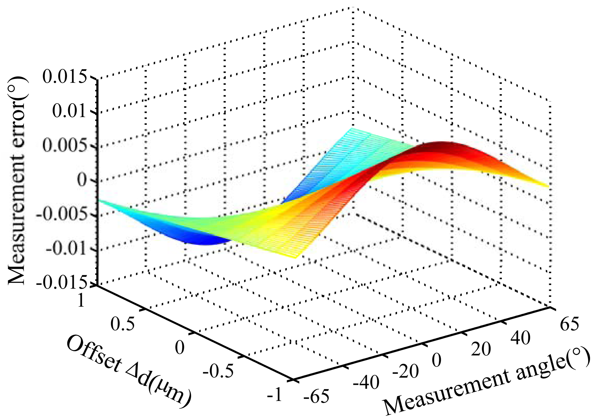
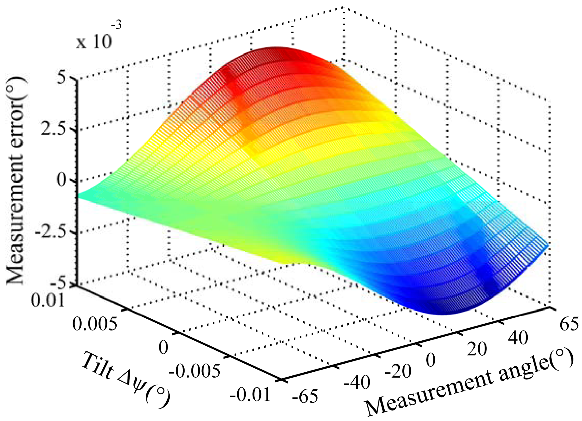
Measurement errors caused by offset (Δd) and tilt (Δφ) deviation for product A and B are analyzed by simulation. The tilt deviation is set as ±0.01°. The offset deviation is set as ±1 micron. Figures 5–7 show the simulation result for product A.
Simulation results show the following:
Measurement errors caused by offset and tilt deviation increase when the distance between entrance slit and code dial decreases or the incident angle increases.
Offset deviation causes more significant measurement errors. For product A, the measurement error will exceed 0.014° when Δd reaches 1 μm, as shown in Figure 5. Therefore, the measurement error caused by offset deviation should not be ignored.
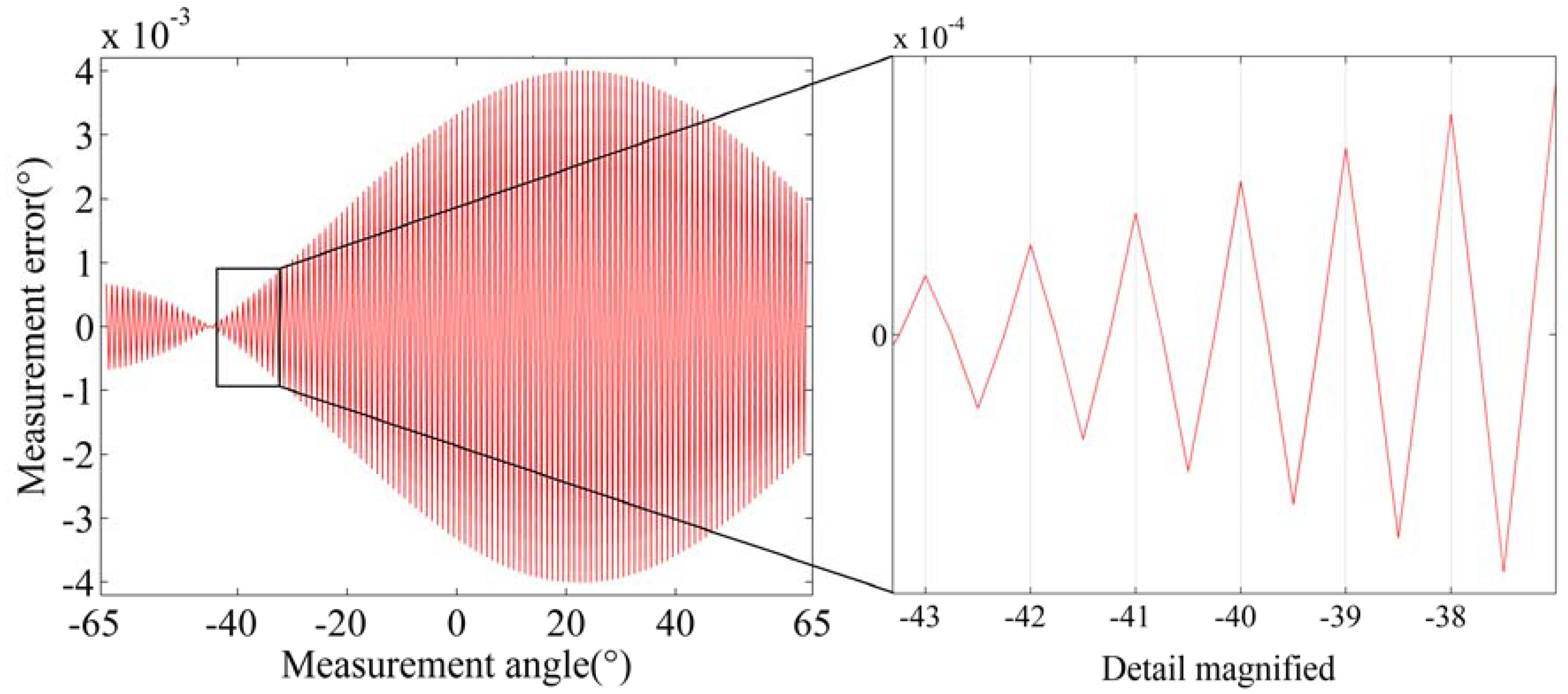
Tilt deviation has relatively less impact on the measurement errors. For product A, the measurement error is less than 0.005° at Δφ = 0.01°, as shown in Figure 6. For product B, the measurement error is much less. Meanwhile, the measurement error caused by Δφ varies with a period of 1° when the measurement angle is increased at 0.5° intervals in the simulation, as shown in Figure 7.
3.3. Algorithm Approximation Error in Signal Processing for Fine-Code
The encoded code dial includes coarse-code rows and fine-code rows. The final output angle is the sum of coarse-code output and fine-code output. The resolution of the ESS depends on the amount of code rows. The more the amount of code rows, the higher the resolution, but the highest resolution of coarse-code rows is only about 0.5°, which is limited by the divergence angle of the sun (0.53°). To improve the resolution further, fine-code rows is added to the code dial. Fine-code rows are not designed by dividing the coarse-code rows into smaller granularity, but adopting the principal that the output signal from the fine-code rows is a specific function of the incident angle α. The output angle of the fine-code can be derived by further processing the output of all fine-code rows. Typically, there are seven coarse-code rows and four fine-code rows. The four fine-code rows have the same pattern, while there is a phase difference of θ0/4 between two adjacent rows. θ0 is the period of fine-code, which is usually designed as 2°. For coarse-code output, an accuracy of 0.5° can be guaranteed. So the signal processing error of fine-code is the primary contributor to the algorithm error of ESS. Ideally, the output current of quad fine-code rows (F1∼F4) can be expressed as:
However, the actual output current of the quad fine-code rows does not follow the above formulas exactly [7]. Instead, they are periodic function similar to sine or cosine. It is well known that any periodic function can be expressed by Fourier series, so the actual output current of the quad fine-code rows can be expressed by Fourier series as:
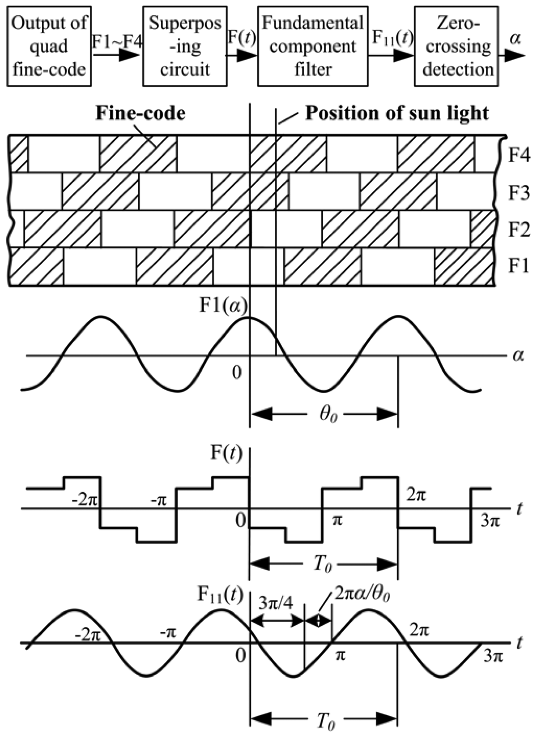
The fine-code signal processing circuit is based on a four-quadrant chopper. The working principle is shown in Figure 8. First, the fundamental components from the four fine-code rows are added together to get a superposed signal (designated as F(t)). Then, the harmonic component in the superposed signal F(t) is eliminated by a filter to get the fundamental component. Finally, an output which is related with the measurement angle α can be achieved by zero crossing detection.
If the output current of the quad fine-code rows is ideal, as shown in Equation (1), the fundamental component F11(t) of superposed signal F(t) should be in the following form:
The relation between the zero-crossing phase ωt0 of the F11(t) and measurement angle α can be deduced by solving the equation of F11(t) = 0:
It can be seen that ωt0 is proportional to α, and there is a fixed phase difference of 3π/4. The phase difference can be compensated by a properly configured gate circuit. The proportional relationship between ωt0 and α is the theoretical base for the fine-code signal processing circuit.
The analysis above is based on the assumption that the output current of the quad fine-code rows is ideal, but from the actual output current shown in Equation (2), it is known that besides the fundamental component and the DC component, there are harmonic components. Among these harmonic components, even harmonics that have nothing to do with the measurement angle, while odd harmonics can bring errors to the measurement. Especially, the third harmonic can bring about a significant error because its amplitude is highest among the odd harmonics. Taking the third harmonic component into consideration, the corresponding fundamental component of superposed signal F(t) becomes:
Compared with Equation (3), the fine-code algorithm error ε caused by the third harmonic can be deduced and expressed as:
In actual design, the fundamental component is always much larger than the harmonic components. That is a3/a1 ≪ 1, so the equation above can be simplified to:
3.4. Errors Introduced By the Etching Process and Non-Uniform Response of Photocell
Manufacturing errors in the etching process will result in amplitude and phase errors of the output current of fine-code rows. The non-uniform response of photocells will cause amplitude errors in the output current of fine-code rows [5]. Generally, these errors are less than ±1% on the average.
3.5. Classification of ESS Errors
From the analysis above, it can be seen that errors in ESS can be classified into three categories:
Structural errors: these include distance deviations between entrance slit and code dial and offset and tilt deviations between the entrance slit and center line of the code dial. These errors belong to the system error class and are invariable. A model can be established to compensate them.
Algorithm approximation errors of the fine-code: the errors are invariable too. A model can be deduced to compensate for them.
Errors introduced by the etching process and non-uniform response of the photocell: the impact of this kind of error is insignificant. Furthermore, to establish a simple model is not easy because they are random errors.
4. Error Compensation Model for ESS
Based on the result of error analysis, the following compensation model for ESS is established. According to the fine-code algorithm error in Equation (8) and the phase error of fine-code output current, the fine-code algorithm error can be fitted by a sine function with parameters k and t as follows:
As analyzed in Sections 3.1 and 3.2, structural errors mainly come from deviations in manufacturing and assembly. Structural errors can be deduced and calculated following the process of imaging (i.e., the process of coordinate transformation from the sunlight incident plane to the angle output in the code dial reference frame).
Suppose the sunlight incident angle is α. Ideally, the sunlight incidence plane can be expressed as:
Taking structural errors (mentioned in Section 3.1 and 3.2) into consideration, the coordinate of the intersection of the incident plane and Y axis can be expressed as:
The corresponding incident angle in the code dial reference frame can be expressed as:
According to the fine-code algorithm error shown in Equation (9) and the structural error shown in Equation (12), the error compensation model for ESS can be expressed as:
5. Calibration of Parameters of the Error Compensation Model
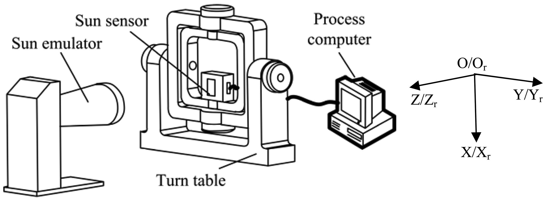
After the error compensation model is established, the model parameters can be calibrated with the equipment shown in Figure 9. The ESS is mounted on the inner-frame of a turntable, and sunlight is provided by a sun emulator. Rotating the inner-frame and external frame of the turn-table by angles α and β respectively have the same effect as sunlight projecting onto the ESS with an incident angle α and incoming angle β. Here, the incoming angle is the intersection angle between the sunlight and the YZ plane of the ESS. Measurement results will be sent to a computer for processing. The turntable will be rotated to m sets of predefined calibration angles. These m sets of angles (αi = 1∼m, βi = 1∼m) and its corresponding ESS outputs αci = 1∼m form an array of calibration data [8,9].
For convenience, the turntable reference frame Or-XrYrZr is defined in the following way: when the turntable is at the zero position, the inner-frame rotation axis is Xr, and the external-frame rotation axis is Yr. Axis Zr is defined by the right-hand rule. The ESS reference frame O-XYZ is defined in the following way: the center of the code dial is O, axis X is perpendicular to the code row direction; axis Y is parallel to the code row direction; and axis Z is defined by the right-hand rule.
Suppose the installation deviation is zero in the calibration system, that is: (a) verticality deviation between the optical axis of the solar simulator and the turntable reference frame Or-XrYrZr is zero; (b) deviation between O-XYZ and Or-XrYrZr is zero. Then, the incoming angle β has no relation with the incident angle α and can have any value. A series of predetermined calibration angles can be generated merely by rotating the inner frame at certain intervals, but in reality, installation deviation is unavoidable and incoming angle β and incident angle α are related. The calibration data has to be acquired for different incoming angles in order to guarantee the accuracy of parameter calibration. Furthermore, all calibration data should be acquired at the same initial zero position of the turntable [10,11].
On the other hand, because of the installation deviation of calibration equipment, the calibration accuracy for parameters will be decreased if the calibration is directly according to the ESS error compensation model. Those installation deviations get involved inevitably during the process of parameter calibration. As a result, these external installation errors have to be taken into account to establish the integrated ESS calibration model as shown in Figure 10.
The accurate calibration model for ESS can be expressed as a function containing installation deviation parameters V0 and Rrs as well as error compensation model parameters a, b, c, d, k and t:
In Equation (14), V0 is the verticality deviation vector between sunlight and the turntable reference frame, and is represented by a 3 × 1 vector. Rrs is the installation deviation matrix between the ESS and the turntable, and can be described by a 3 × 3 conversion matrix between the ESS and the turntable reference frame. Terms α and β are the known calibration angles (i.e., rotation angles of the inner and external frames of the turntable, respectively); R(α, β) is the corresponding rotation matrix of the turn-table. f1(a, b, c, d, k, t) is the ESS error compensation function shown in Equations (9) and (13). f2(Rrs, V0) is the function of installation deviation and equal to the product of Rrs and V0.
It can be seen in Equation (14) that there are eighteen parameters that need to be optimized for solutions, namely, (a, b, c, d, k, t, e1, e2, e3) and (r1–r9). Among them, (a, b, c, d, k, t) are the error compensation parameters of the ESS itself, which are defined as internal parameters of the ESS. (e1, e2, e3) and (r1–r9) are installation deviation parameters between the ESS and the calibration equipment, which are defined as external parameters of the ESS. α̅ is the estimated value of ESS output angle calculated by the calibration model.
The calibration data are substituted into the calibration model shown in Equation (14). All parameters (including installation deviation parameters and ESS error compensation parameters) can be optimized by the Least Squares method. The specific optimization procedure is as follows:
Rotated angles of the turntable (αi = 1∼m, βi = 1∼m) are substituted into the calibration model shown in Equation (14) to get the estimated value α̅i=1∼m of the ESS output angle. Combined with the actual value αci = 1∼m, of the ESS output angles, a system of equations containing m equations is formed, as shown in Equation (15).
It can be seen that the Equation (15) is an over-determined equation system involving eighteen parameters. The equation can only be solved by optimization. In the paper, s Nonlinear Least Squares iteration algorithm is used to solve the parameters. The detailed procedure is as follows:
Equation (15) can be expressed in the following vector form:
Based on the nonlinear least squares iteration algorithm, the following iteration equation can be established:
6. Experimental Results
Calibration and accuracy verification experiments are carried out on a large number of products. They are tested within different ranges of incident angles, tested at different sample intervals of incident angle and different installation deviations of the calibration system. The experimental results are shown in Tables 1, 2 and 3. Table 1 shows the statistical results for twenty products randomly selected, which are tested in different ranges of the incident angle.
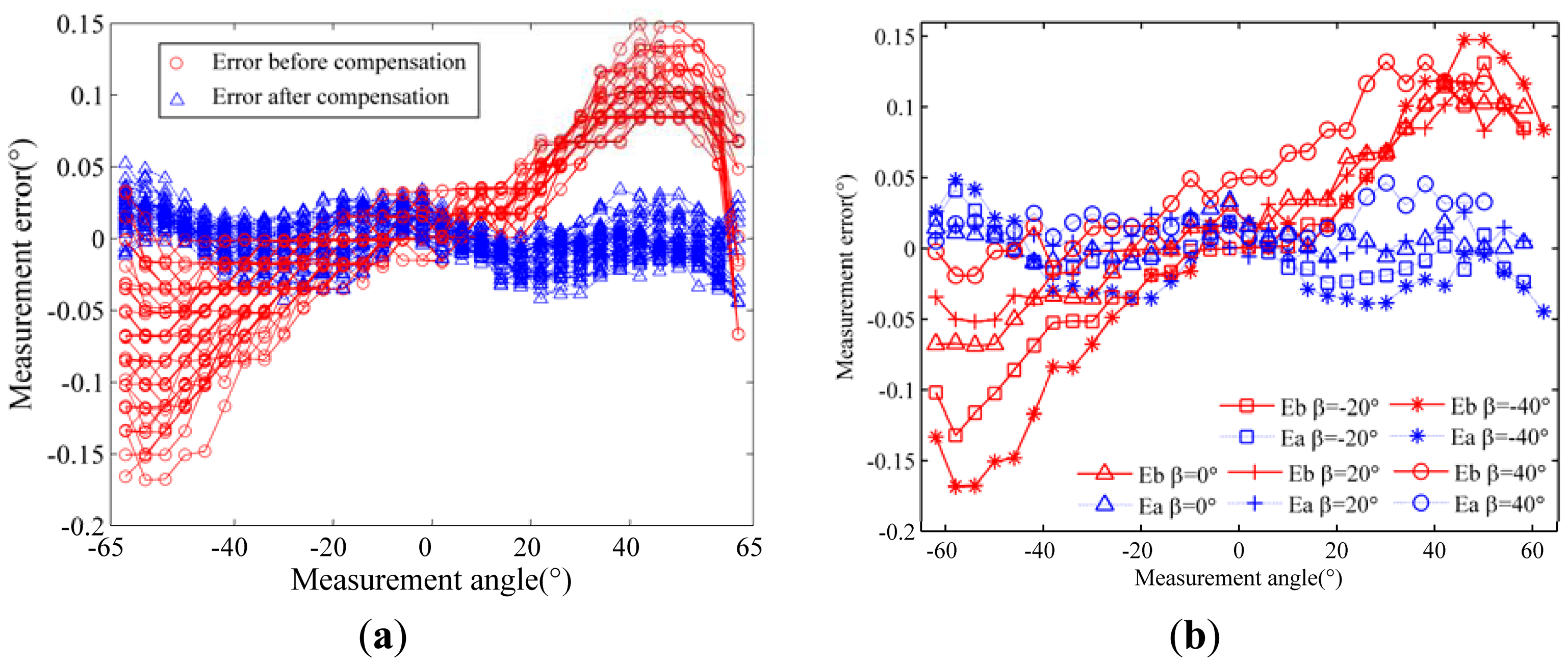
Table 2 shows the results for two products at different sample intervals of the incident angle. Table 3 shows the error compensation parameters calibrated for one product under different installation deviation between ESS and turntable. Figure 11 shows a typical result for one product of type B, whose RMS error is 0.0635° before compensation and 0.0157° after compensation, and whose calibrated parameters are shown in Table 4. Measurement errors before and after compensation are shown in Figure 11(a), in which each curve represents one set of measurement errors for different incoming angles β. For clarity, a few representative curves are selected from (a) and plotted in Figure 11(b), in which “Eb” represents “error before compensation” and “Ea” represents “error after compensation”.
Experimental results show the following:
From Table 1, it can be seen that accuracy improvement is greater within 30° ∼ 60° than that within ±30°, and the accuracy improvement for product A is greater than that for Product B. This is because measurement errors caused by structural errors increase when H decreases or the incident angle increases as analyzed in Section 3.
From Table 2, it can be seen that the compensation effect with a 0.25° sampling interval is better than that with a 1°sampling interval, but the improvement is limited. It agrees with our theoretical analysis, and here are reasons for that:
Because the fine-code algorithm compensation equation is a sine function with a period of 0.5°, the compensation effect is improved when the calibration data is sampled at an interval shorter than the period of 0.5°.
The solved parameter k is generally less than 0.03, which indicates that the impact of the fine-code algorithm error is relatively minor, so there is a limit on the improvement.
From Table 2, it can be seen that the error compensation parameters calibrated under different installation deviations are almost identical, which indicates that the calibration model and method proposed in the paper effectively avoid the impact of installation deviations of the calibration equipment.
From Table 1, it can also be seen that after compensation, the ESS measurement accuracy is improved by three times on average within ±60° of the incidence angle.
7. Conclusion
Various kinds of error in ESS are analyzed in this paper. The result shows that the structural errors which occurred during the manufacturing and assembly processes, together with the algorithm approximation errors of the fine-code, are the major factors which limit the measurement accuracy of ESS units. Based on the analyzed results, an error compensation model is established to compensate the errors mentioned above.
In addition, an accurate parameter calibration method is also proposed. To avoid the impact of installation deviations of the calibration system on the accuracy of parameter calibration, an accurate calibration model of ESS is established which takes the installation deviation of calibration equipment into consideration. The experimental results show that after compensation, the ESS measurement accuracy is improved by three times on average within ±60° of the incidence angle. The technology described in the paper has been successfully applied to sun sensor products of a certain research institute in China.
Acknowledgments
This project is supported by National Science Foundation of China (Grant No. 61008032) and certain research institute in China.
References
- Leijtens, J. Sunsensor Miniaturization Where is the End. Proceedings of IEEE Sensors Conference, Lecce, Italy, 26–29 October 2008; pp. 1348–1351.
- Hales, J.H.; Pedersen, M. Two-Axis MOEMS Sun Sensor for Pico Satellites. Proceedings of 16th Annual AIAA/USU Conference on Small Satellites, Logan, UT, USA, 12–15 August 2002; pp. 1–12.
- Li, W.Y.; Zhang, G.F.; You, Z.; Xing, F. Error compensation for area digital sun sensor. Sensors 2012, 12, 11798–11810. [Google Scholar]
- Wu, S.F.; Steyn, W. Modelling and in-orbit calibration practice of a miniature 2-axis analogue sun sensor. Aerosp. Sci. Technol. 2002, 6, 423–433. [Google Scholar]
- Yu, F.X.; Sun, L.L. Error analysis of pico-satellite attitude angle measurement based on sun vector. J. Jilin Univ. (Eng. Technol. Ed.) 2008, 4, 976–981. [Google Scholar]
- Chen, F.; Li, Y.; Shi, Y. New Sun Sensor and its Test. Proceedings of 2nd International Symposium on Instrumentation Science and Technology, Jinan, China, 18–22 August 2002; pp. 400–403.
- Cosner, C.M.; Barker, D.S. Modeling Analog Sun Sensor Current Output. Proceedings of the First IEEE Regional Conference on Aerospace Control Systems, Westlake Village, CA, USA, 25–27 May 1993; pp. 156–160.
- Yu, C.; Jia, J.; Lv, Z.; Lu, X. Study on Sun CCD Sensor Error Analysis and Calibration Method. Proceedings of 12th National Academic Annual of the Space and Mobile Control Technology, Guilin, China, 11–14 August 2006; pp. 495–499.
- Zhang, G.J.; Wei, X.G.; Fan, Q.Y.; Jiang, J. Method and Device for Calibration of Digital Celestial Sensor. Patent US7822572, 2010. [Google Scholar]
- Strietzel, R. Two-Dimensional Calibration of a Sun Attitude Sensor. Proceedings of 15th International Federation of Automatic Control Triennial World Congress on Automatic Control, Barcelona, Spain, 21–26 July 2002; pp. 259–264.
- Xiong, X.P.; Wang, C.K. Measuring device for output error of the solar sensor. Sci. Guide 2009, 19, 38–41. [Google Scholar]


| Product Type | Range of Incident Angle | RMS Error after Compensation | Times of Accuracy Improvement | |||
|---|---|---|---|---|---|---|
| Max | Min | Mean | Max | Min | ||
| Type A (H = 4.124 mm) | ±30° | 0.0113° | 0.0071° | 4.76 | 6.04 | 3.25 |
| ±30°∼±60° | 0.0229° | 0.0099° | 5.526 | 6.8 | 3.96 | |
| ±62° | 0.0245° | 0.0093° | 3.94 | 5.17 | 2.7 | |
| Type B (H = 6.584 mm) | ±30° | 0.010° | 0.005° | 2.88 | 4.5 | 1.49 |
| ±30°∼±60° | 0.0143° | 0.0073° | 4.47 | 5.18 | 3.07 | |
| ±62° | 0.157° | 0.0056° | 3.34 | 4.27 | 2.83 | |
| Product Type | Sample Interval | Range of Incident Angle | RMS Error before Compensation | RMS Error after Compensation |
|---|---|---|---|---|
| Type A (H = 4.124 mm) | 1° | ±62° | 0.0399° | 0.0141° |
| 0.25° | ±62° | 0.0296° | 0.0102° | |
| Type B (H = 6.584 mm) | 1° | ±62° | 0.020° | 0.007° |
| 0.25° | ±62° | 0.0191° | 0.0056° | |
| Deviation Between O-XYZ and Or-XrYrZr | Error Compensation Parameters | |||||||
|---|---|---|---|---|---|---|---|---|
| Axis X | Axis Y | Axis Z | a | b | c | d | k | t |
| 0 | 0 | 0 | 4.1289 | −0.0003 | −0.0003 | 4.1191 | −0.0225 | −0.7787 |
| 0 | 5′ | 38″ | 4.1292 | −0.0001 | −0.0002 | 4.1188 | −0.0164 | −0.8623 |
| 17″ | 1′34″ | 1′8″ | 4.1289 | −0.0003 | −0.0004 | 4.1191 | −0.0177 | −0.8005 |
| a | b | c | d | k | t | r1 | r2 | r3 |
|---|---|---|---|---|---|---|---|---|
| 6.5912 | −0.0005 | −0.0006 | 6.5759 | 0.0357 | 2.4558 | 1.0000 | 0.0004 | 0.0014 |
| r4 | r5 | r6 | r7 | r8 | r9 | e1 | e2 | e3 |
| −0.0004 | 1.0000 | −0.0003 | −0.0014 | 0.0003 | 1.0000 | −0.0066 | 0.0001 | 1.0000 |
© 2013 by the authors; licensee MDPI, Basel, Switzerland. This article is an open access article distributed under the terms and conditions of the Creative Commons Attribution license (http://creativecommons.org/licenses/by/3.0/).
Share and Cite
Fan, Q.; Zhang, G.; Li, J.; Wei, X.; Li, X. Error Modeling and Calibration for Encoded Sun Sensors. Sensors 2013, 13, 3217-3231. https://doi.org/10.3390/s130303217
Fan Q, Zhang G, Li J, Wei X, Li X. Error Modeling and Calibration for Encoded Sun Sensors. Sensors. 2013; 13(3):3217-3231. https://doi.org/10.3390/s130303217
Chicago/Turabian StyleFan, Qiaoyun, Guangjun Zhang, Jian Li, Xinguo Wei, and Xiaoyang Li. 2013. "Error Modeling and Calibration for Encoded Sun Sensors" Sensors 13, no. 3: 3217-3231. https://doi.org/10.3390/s130303217