As one important branch of modern array signal processing, the beamforming technique has been widely studied and applied in the radar, wireless communication, sonar, medical imaging, as well as astronomy domains. The standard beamforming approach, such as the minimum variance distortionless response (MVDR) beamformer [1], was usually established based on an ideal antenna array with exactly known array manifold. Thus, it is very sensitive to practical circumstances, and its performance would be seriously degraded by diverse factors, such as the steering vector mismatch, array calibration errors and snapshot number restrictions.

During the last decades, in order to resist the model mismatches and possible environment changes, the robust beamforming approach have been largely studied [2–5]. Among others, by introducing a penalty term into the objective function, the diagonal loading (DL) algorithm could effectively reduce the eigenvalue spread of the noise and prevent the distortion of beampattern [6]. Nevertheless, how to get the optimal loading factor for DL is still a serious issue when the desired steering vector and/or the available snapshot numbers are uncertain [7]. A robust adaptive beamforming, based on the worst-case performance optimization, would delimit the uncertainty set of steering vectors by upper bounding the norm of the steering vector mismatch [8]. However, neither the mismatch vector nor its upper bound is known in practice. To overcome this model defect in standard DL algorithm, an adaptive beamforming method was developed, which estimates iteratively the difference between the actual and presumed steering vectors in order to maximize the output signal-to-noise plus interference ratio (SINR) [9–11]. But this adaptive beamforming algorithm is not sufficiently reliable in the case when the snapshots are small.

In order to reject jamming signals, poor array calibration, signal wave-front distortions, the minimum-variance-distortionless-response (MVDR) beamforming is modified by the means of incorporating multiple linear constrains [12–14]. Whereas, the augmentation of constrains would reduce the array freedom degrees in the linear beamforming framework. Nonlinear beamforming approaches provide a novel idea to address this issue for they can adapt better to the statistical properties of the given data than linear ones [15]. Neural network has been applied to beamforming among other nonlinear array processing tasks. But this approach suffers from serious drawbacks such as over-fitting or local minima, which leads to suboptimal solutions [16].

Support Vector Machines (SVM), introduced by Vapnik [17], is an important new methodology for pattern classification and nonlinear function approximation. This method addresses the beamforming problem by means of incorporating additional inequality constrains to penalize sidelobe levels and allowing a certain error in the desired signal direction [18]. Thus the MVDR beamforming method is reformulated and the cost function turns out to be equivalent to SVM for regression. However, the time consumed to train SVM beamformer scales super linearly to the number of observations, and it leads to an insurmountable computational burden in online operation modes [19]. The least-squares support vector machine (LS-SVM) inherits the SVM's generalization capacity. By solving linear equations instead of a quadratic programming (QP) problem in the standard SVM, the training procedure and the computational complexity of the standard SVM would be effectively simplified [20]. The main drawback of LS-SVM is that it works in batch mode. Thus, it is difficult to be used in large-scale applications. Recent researches about LS-SVM continuously focus on the improvement of the training algorithms, model selection and sparseness [21,22].

This paper presents a new LS-SVR-based approach to address the robust beamforming issue. This approach alleviates the array output SINR degradation in the presence of steering vector mismatches, strict restrictions on the number of available snapshots, and numerous interferences by replacing the conventional linearly constrained minimum variance cost function with a squared-loss function, and achieves better generalization capacity by applying Gaussian kernels to the array observations. We also present a fast recursive procedure to estimate the weight vectors on real-time, and a novelty criterion to perform model reduction. The paper is organized as follows. The signal model, also the minimum mean square error (MMSE) and the MVDR-beamformer solutions are presented in Section 2. The basic principle of LS-SVR-based beamforming method is introduced in Section 3. In Section 4, a recursive procedure to calculate the regression parameters is provided. And a sparse mode is presented in Section 5. The simulation tests under different mismatch scenarios are illustrated in Section 6. A summary conclusion is given at the last of this paper.

Consider a linear array of M sensors receives signals from D narrowband source. The vector of array observations x(t) ∈ C^M×1 at time t could be modeled as: (1) x ( t ) = A s ( t ) + n ( t )where, θ = [θ₁, θ₂,…, θ_D]^T ∈ R^D×1 is the vector with the directions of arrival (DOA) and (·)^T stands for transpose, A = [a(θ₁), a(θ₂)…a(θ_D)] ∈ C^M×D is the matrix containing the array steering vectors a (θ_i) = [1,e^{−j2πsin(θi)d/λ}…e^{−j2πsin(θi)d/λ}]^T. The uncorrelated sources are represented by the vector s(t) = [s₁(k), s₂(k))…s_D(k)]^T ∈ C^M×1. The vector n(t) ∈ C^M×1 is the sensor noise, and it is assumed as complex Gaussian with zero-mean: (2) A = [ a ( θ 1 ) , a ( θ 2 ) ⋯ a ( θ D ) ]

The output of the beamformer is defined as: (3) y ( t ) = w H x ( t )where, w = [w₁, …, w_M]^T ∈ C^M×1 is the complex vector of beamformer weights, (·)^T denotes transpose, and (·)^H denotes Hermitian transpose.

If certain observations are known during the procedure of training parameters, then, according to the MMSE criterion, the complex vector of beamformer weights w can be described as: (4) w = R − 1 pwhere, R is M × M covariance matrix, and p is the cross-correlation between the desired output and the received signal.

The classical MVDR beamformer minimizes the array output energy, and the weights subject to a constraint of unity array response on the desired array steering vectors, that is: (5) min w w H R w s . t . w H a ( θ 1 ) = 1

The constraint w^Ha(θ₁) = 1 prevents the gain at the look direction from being reduced, and the solution of Equation (5) can be easily estimated by means of using Largrange multiplier method: (6) w = R − 1 a ( θ 1 ) a ( θ 1 ) H R − 1 a ( θ 1 )

In practice, it is not feasible to calculate the exact covariance matrix R and it would be estimated by the sample covariance matrix R ^ = 1 K ∑ k = 1 K x ( k ) x H ( k ) where K is the number of observed snapshots.

The performance of MVDR beamformer in Equation (5) is sensitive to mismatch between the presumed and actual steering vectors due to the uncertainty of the desired signal DOA, strict restrictions on the number of available snapshots, and numerous interferences.

From Equation (16), it could be known that once the regression parameters α_t and b_t are computed, the beamformer outputs can be obtained. Denoting U_t = H_t⁻¹ = (Q_t + C⁻¹I)⁻¹, the result of LS-SVR (Equation (14)) can be represented as: (17) [ 0 e ¯ T e ¯ U t − 1 ] [ b t α t ] = [ 0 y ¯ t ]

Then, we have: (18) b t = e T U t y t e T U t e α t = U t ( y t − e e T U t y t e T U t e )

As the number of snapshots increases, the dimension of Gramm matrix Q_i will be increasing because it is in proportional to the number of snapshots. Therefore, the computation for the regression parameters α_t and b_t would be very intensive as the snapshots increase, and it is key issue for LS-SVR beamformer to find out a fast algorithm to improve the computation efficiency of U_i.

At time step t, Q_i and H_i are the matrixes with dimension of 2N × 2N: (19) Q t = ( k ( x ¯ 1 , x ¯ 1 ) ⋯ k ( x ¯ t , x ¯ 1 ) ⋮ ⋮ ⋮ k ( x ¯ 1 , x ¯ t ) ⋯ k ( x ¯ t , x ¯ t ) ) H t = ( Q t + C − 1 I ) = ( k ( x ¯ 1 , x ¯ 1 ) + 1 / C … k ( x ¯ 2 N , x ¯ 1 ) ⋮ ⋱ ⋮ k ( x ¯ 1 , x ¯ 2 N ) ⋯ k ( x ¯ 2 N , x ¯ 2 N ) + 1 / C )

As time run to t + 1, new input snapshots x_t+1 and the corresponding desired array output y_t+1 are added to the current training set. So Q_t+1 and H_t+1 can be represented as: (20) Q t + 1 = ( k ( x ¯ 1 , x ¯ 1 ) … k ( x ¯ 2 N , x ¯ 1 ) k ( x ¯ 2 ( N + 1 ) , x ¯ 1 ) ⋮ ⋱ ⋮ ⋮ k ( x ¯ 1 , x ¯ 2 N ) ⋯ k ( x ¯ 2 N , x ¯ 2 N ) k ( x ¯ 2 ( N + 1 ) , x ¯ 1 ) k ( x ¯ 1 , x ¯ 2 ( N + 1 ) ) ⋯ k ( x ¯ 2 N , x ¯ 2 ( N + 1 ) ) k ( x ¯ 2 ( N + 1 ) , x ¯ 2 ( N + 1 ) ) ) H t + 1 = Q t + 1 + C − 1 I = ( k ( x ¯ 1 , x ¯ 1 ) + 1 / C ⋯ k ( x ¯ 2 N , x ¯ 1 ) k ( x ¯ 2 ( N + 1 ) , x ¯ 1 ) ⋮ ⋱ ⋮ ⋮ k ( x ¯ 1 , x ¯ 2 N ) ⋯ k ( x ¯ 2 N , x ¯ 2 N ) + 1 / C k ( x ¯ 2 ( N + 1 ) , x ¯ 1 ) k ( x ¯ 1 , x ¯ 2 ( N + 1 ) ) ⋯ k ( x ¯ 2 N , x ¯ 2 ( N + 1 ) ) k ( x ¯ 2 ( N + 1 ) , x ¯ 2 ( N + 1 ) ) + 1 / C )

Comparing the elements of H_t and H_t+1, the matrix H_t+1 could be reconstructed by the matrix H_t plus an additional row and column, i.e., (21) H t + 1 = ( H t v t + 1 v t + 1 T v t + 1 )where, v_t+1 = [k(x̄₁, (x̄_2(N+1)), … k(x̄_2N, (x̄_2(N+1))]^T, v_t+1 = k(x̄_2(N+1)), x̄_2(N+1)) + 1/C).

According to the theorem of inverting block matrix, the inverse of H_t+1 can be expressed by the inverse of H_t and the new column v_t+1 as: (22) H t + 1 − 1 = ( H t − 1 + β H t − 1 v t + 1 v t + 1 T H t − 1 − β H t − 1 v t + 1 − β v t + 1 T H t − 1 β )where, β = ( v t + 1 − v t + 1 T H t − 1 v t + 1 ). Thus the inverse of H_t+1,which is equal to U_t+1, can be calculated from the inverse of H_t, and it is not necessary to calculate the inverse of H_t when it has high dimension, so the computation complexity would be greatly reduced and the numerical stability problem arising from inverse matrix would be also avoided. When the set of snapshots is small, the U_t can be computed directly by matrix inverse theory.

The crucial drawback of LS-SVR beamformer is that it deals with high-dimension matrix, which is equal to the number of the snapshots due to the use of a quadratic constraint function. This would bring a big implementation problem to the proposed beamforming method since it is required to increase memory and computational resources as time evolves. Several methods have been proposed to cope with these problems [23,24]. The sliding-window approach [25] fixes the size of LS-SVR beamformer and allows it to be operated online in time-varying environments by keeping only the last N input snapshots in the sliding-window and simply abandoning those out of it. In [26], an exponential forgetting mechanism is introduced to describe the influence, which is imposed on the present situation by the past data [26]. This paper employs the novelty criterion, presented by Platt [27,28], to reduce the final size of the proposed beamformer, keep the algorithm complexity bounded and realize online sparsification. The basic idea of this approach is to construct a dictionary with center set C and update it appropriately according to the novelty criterion. The stages of the proposed specification are given as follows:

Step 1: Initialing an empty center set C₀;

Increasing δ₁ and δ₂, the final size of the LS-SVR beamformer will be decreased. But this will result to performance degradation. In practical applications, δ₁ is set to around one tenth of the kernel bandwidth, and δ₂ is around the square root of the steady-state mean square error (MSE). Cross-validation also can be used to select these appropriate thresholds.

Applying the above sparsification procedure, the computation complexity of the proposed beamformer will be reduced from O(N²) to O(K²), where K is the effective number of centers in the network at time t. As K is finite, the online real-time beamforming will be practical.

To evaluate the performance of the proposed LS-SVR-based beamformer, simulation tests are carried out. A 10 elements uniform linear array with half-wavelength spacing is taken into account. The desired signal comes from a presumed direction θ = 3° and two irrelevant interferences, with interference-to-noise ratio (INR) of 20 dB, impinge on the array from θ₂ = −32° and θ₃ = 17° respectively. The additive noise is assumed to be a 0-dB complex white Gaussian distributed random variable. For comparison purpose, the conventional MVDR, the diagonal loading MVDR (MVDR-DL), the ES [29], the SQP [9] and the RR [30] method are considered. The parameters of the proposed beamformer, σ, δ₁ and δ₂, are chosen as 1.0, 0.1 and 0.08 respectively. The load value of MVDR-DL beamformer is set to (P_e+10 dB), where P_e denotes the power of desired signal. All results are obtained from 100 independent simulation runs.

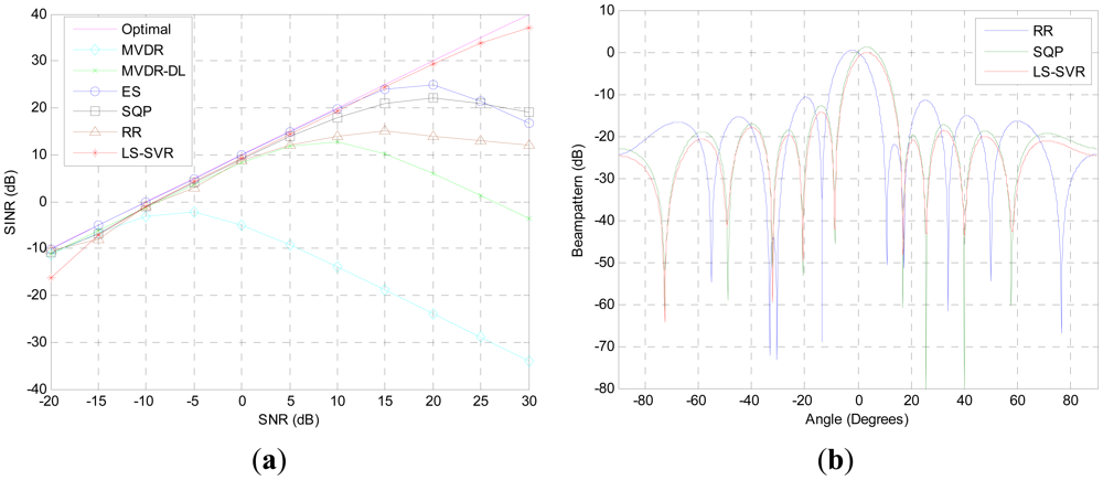
The first simulation aims to compare the performance of these beamformers when steering vector mismatch is presented. From Figure 1(a), we observe that the proposed LS-SVR beamformer consistently improves its output SINR as SNR increases and performs much closer as the idea one when the input SNR is varied from −20 dB to 30 dB. Due to the DOA mismatch, the interested signal is considered as interference and a null is allocated in the desired signal direction by the MVDR beamformer. As a result, the output SINR is decreased. When input SNR is larger than −5 dB, the output SINR of MVDR beamformer degrades seriously. In comparing with the MVDR beamformer, the MVDR-DL, ES, SQP and RR methods get more robustness against DOA mismatch. But they still suffer from a degradation of performance while the input SNR becomes higher.

Figure 1(b) shows the normali\zed beampattern plots when the input SNR is equal to 10 dB. As it is illustrated, all beam-patterns of the robust beamformers have nulls at the DOAs of the interferences. But the proposed LS-SVR still outperforms others by markedly lower sidelobe level, and maintaining distortionless response for the desired signal.

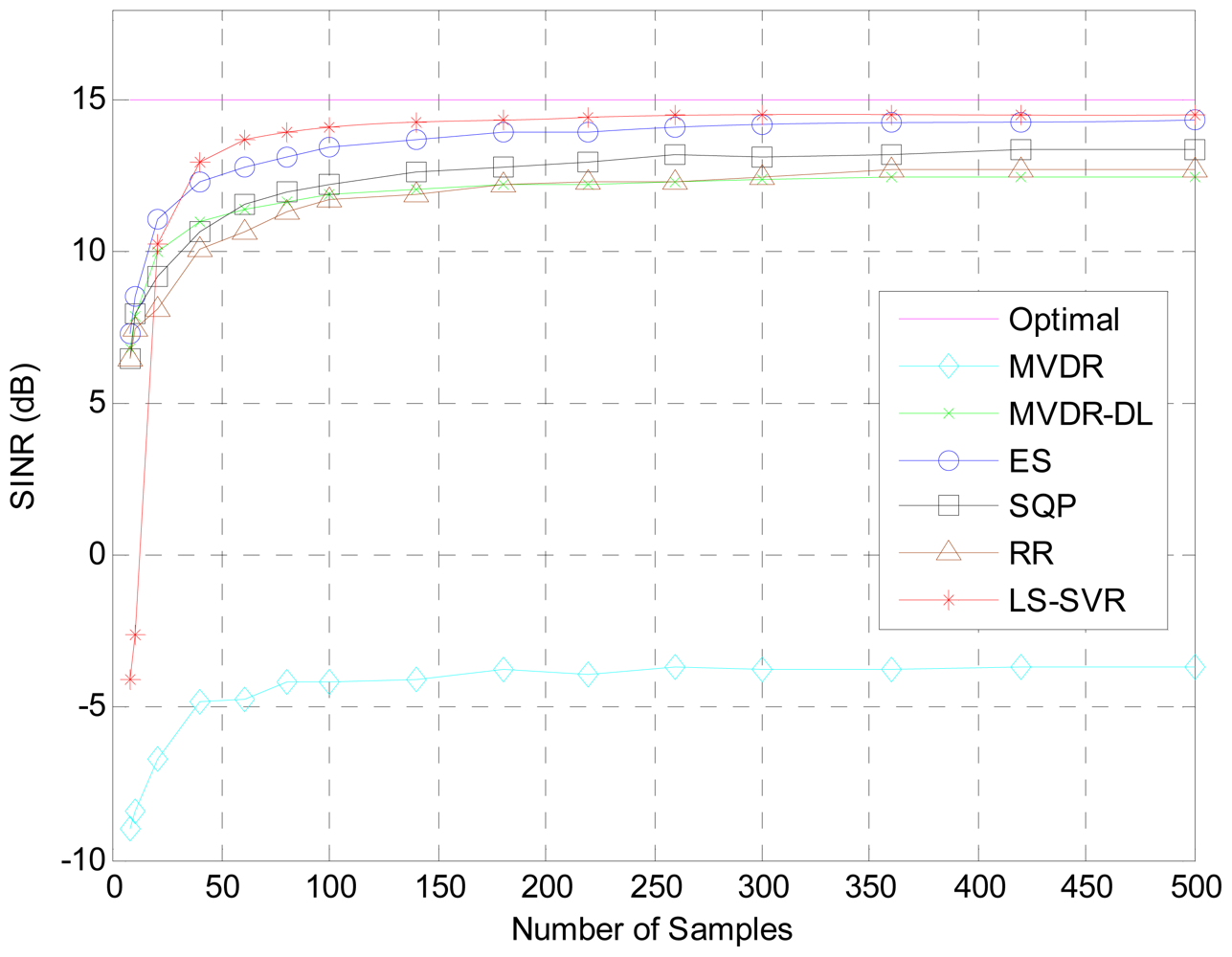
The covariance matrix would be inaccurately estimated owing to insufficient snapshots, DOA mismatch of desired signal and array calibration errors. This kind of inaccuracy may result in the degradation of array response. Hence, both the errors of insufficient snapshots and DOA mismatch are considered to verify the proposed beamformer in our second simulation tests. Figure 2 shows the resulting output SINRs versus the snapshot number K. When snapshots are over 20, the LS-SVR clearly outperforms other beamformers tested. Owing to the steering vector mismatch, the MVDR beamformer see the desired signal as interference and fails in its operation.

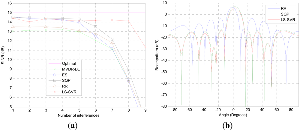
The performance of the proposed beamformer in the scenario with multiple interferences is demonstrated in the third test. The steering vector mismatch is also presented. As it can be seen from Figure 3(a), the proposed algorithm performs equally well as ES and SQP when the number of interferences less than 5. When the interference numbers is increased to 8, the output SINR of the proposed LS-SVR beamformer is only 1 dB lower than that of idea beamformer. In contrast, the output SINRs of other beamformers tested are dramatically decreased due to the decrease of the available freedom degrees which are devoted to suppress the interference.

The corresponding beampatterns of the beamformers are demonstrated in Figure 3(b), where the four interferences with DOAs of θ_i = [17.4°, −11.5°, 53.1°, −23.5°] are taken into account. It can be seen that the LS-SVR beamformer not only presents deep nulls at the DOAs of interference, but also achieves better sidelobe suppression than other beamformers tested. Thus, the proposed LS-SVR method can get better SINR performance than the usual robust linear beamforming algorithms in the case of numerous interferences.

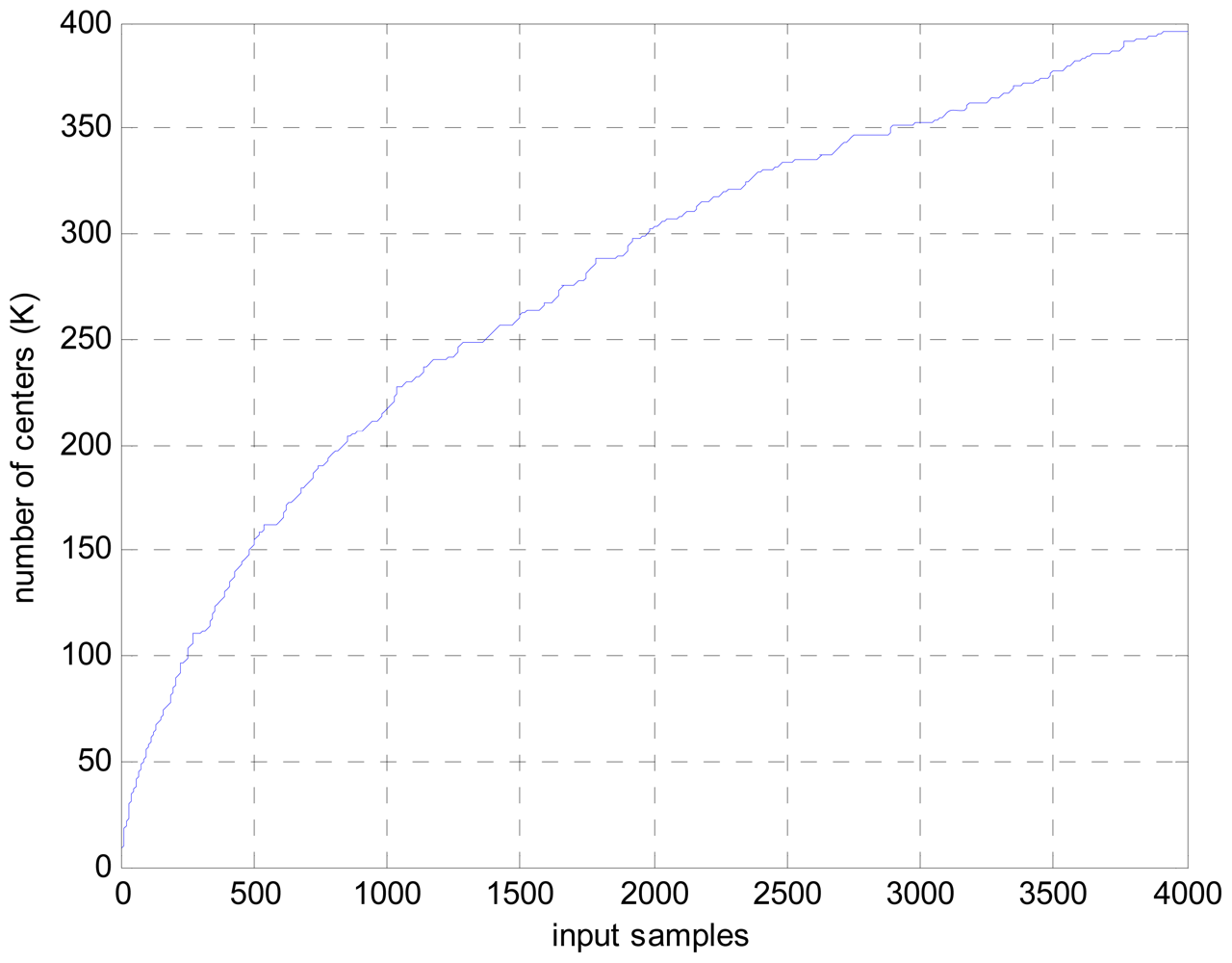
To show the computation complexity of the novel approach, the dictionary size growth with the input samples is given in Figure 4. As it can be seen in Figure 4, only 396 center numbers are needed to calculate the beamformed output for 4,000 input samples. In comparison with the original LS-SVR algorithm, in which 4,000 centers are needed for the same case. Thus, the computation cost is largely reduced.

We present a novel nonlinear LS-SVR-based beamforming approach in this paper. This approach first uses a squared-loss function to replace the conventional linearly constrained minimum variance cost function, which can significantly increase robustness against mismatch problems and provide additional control over the sidelobe level. The method also applies Gaussian kernels to the array observations to improve the generalization capacity. Finally, the method uses a recursive regression procedure to estimate the weight vectors on real-time and performs mode reduction to reduce the final size of the beamformer.

The simulation tests, with steering vector mismatch, numerous interferences and limited available snapshots, are carried out to verify the performance of the proposed beamforming algorithm in comparison with other recently proposed ones. The test results show that the proposed beamforming method significantly outperforms many other recently proposed linear robust beamforming techniques in terms of signal distortion in the desired signal and noise reduction in scenarios with DOA mismatch, limited observation samples, and numerous interferences.