<?xml version="1.0" encoding="UTF-8"?>
<!DOCTYPE article PUBLIC "-//NLM//DTD Journal Publishing DTD v2.3 20070202//EN" "journalpublishing.dtd">
<article xmlns:mml="http://www.w3.org/1998/Math/MathML" xmlns:xlink="http://www.w3.org/1999/xlink" xml:lang="en" article-type="research-article">
<front>
<journal-meta>
<journal-id journal-id-type="publisher-id">Sensors</journal-id>
<journal-title>Sensors</journal-title>
<issn pub-type="epub">1424-8220</issn>
<publisher>
<publisher-name>Molecular Diversity Preservation International (MDPI)</publisher-name></publisher></journal-meta>
<article-meta>
<article-id pub-id-type="doi">10.3390/s120811221</article-id>
<article-id pub-id-type="publisher-id">sensors-12-11221</article-id>
<article-categories>
<subj-group>
<subject>Article</subject></subj-group></article-categories>
<title-group>
<article-title>Complete Scene Recovery and Terrain Classification in Textured Terrain Meshes</article-title></title-group>
<contrib-group>
<contrib contrib-type="author">
<name><surname>Song</surname><given-names>Wei</given-names></name><xref ref-type="aff" rid="af1-sensors-12-11221"><sup>1</sup></xref></contrib>
<contrib contrib-type="author">
<name><surname>Cho</surname><given-names>Kyungeun</given-names></name><xref ref-type="aff" rid="af1-sensors-12-11221"><sup>1</sup></xref><xref ref-type="corresp" rid="c1-sensors-12-11221"><sup>*</sup></xref></contrib>
<contrib contrib-type="author">
<name><surname>Um</surname><given-names>Kyhyun</given-names></name><xref ref-type="aff" rid="af1-sensors-12-11221"><sup>1</sup></xref></contrib>
<contrib contrib-type="author">
<name><surname>Won</surname><given-names>Chee Sun</given-names></name><xref ref-type="aff" rid="af2-sensors-12-11221"><sup>2</sup></xref></contrib>
<contrib contrib-type="author">
<name><surname>Sim</surname><given-names>Sungdae</given-names></name><xref ref-type="aff" rid="af3-sensors-12-11221"><sup>3</sup></xref></contrib></contrib-group>
<aff id="af1-sensors-12-11221">
<label>1</label> Department of Multimedia Engineering, Dongguk University-Seoul, 26 Pildosng 3 Ga, Jung-gu, Seoul 100-715, Korea; E-Mails: <email>songwei@dongguk.edu</email> (S.W.); <email>khum@dongguk.edu</email> (K.U.)</aff>
<aff id="af2-sensors-12-11221">
<label>2</label> Division of Electronics and Electrical Engineering, Dongguk University-Seoul, 2 Pildong 3 Ga, Jung-gu, Seoul 100-715, Korea; E-Mail: <email>cswon@dongguk.edu</email></aff>
<aff id="af3-sensors-12-11221">
<label>3</label> Agency for Defense Development, Bugyuseong daero 488 beon gi, Yoseong, Daejeon 305-152, Korea; E-Mail: <email>sdsim@add.re.kr</email></aff>
<author-notes>
<corresp id="c1-sensors-12-11221">
<label>*</label>Author to whom correspondence should be addressed; E-Mail: <email>cke@dongguk.edu</email>; Tel.: +82-10-9070-9342; Fax: +82-2-2260-3766.</corresp></author-notes>
<pub-date pub-type="collection">
<year>2012</year></pub-date>
<pub-date pub-type="epub">
<day>13</day>
<month>08</month>
<year>2012</year></pub-date>
<volume>12</volume>
<issue>8</issue>
<fpage>11221</fpage>
<lpage>11237</lpage>
<history>
<date date-type="received">
<day>16</day>
<month>07</month>
<year>2012</year></date>
<date date-type="rev-recd">
<day>07</day>
<month>08</month>
<year>2012</year></date>
<date date-type="accepted">
<day>07</day>
<month>08</month>
<year>2012</year></date></history>
<permissions>
<copyright-statement>© 2012 by the authors; licensee MDPI, Basel, Switzerland.</copyright-statement>
<copyright-year>2012</copyright-year>
<license>
<p>This article is an open access article distributed under the terms and conditions of the Creative Commons Attribution license (http://creativecommons.org/licenses/by/3.0/).</p></license></permissions>
<abstract>
<p>Terrain classification allows a mobile robot to create an annotated map of its local environment from the three-dimensional (3D) and two-dimensional (2D) datasets collected by its array of sensors, including a GPS receiver, gyroscope, video camera, and range sensor. However, parts of objects that are outside the measurement range of the range sensor will not be detected. To overcome this problem, this paper describes an edge estimation method for complete scene recovery and complete terrain reconstruction. Here, the Gibbs-Markov random field is used to segment the ground from 2D videos and 3D point clouds. Further, a masking method is proposed to classify buildings and trees in a terrain mesh.</p></abstract>
<kwd-group>
<kwd>mobile robot</kwd>
<kwd>terrain reconstruction</kwd>
<kwd>multisensor integration</kwd>
<kwd>Gibbs-MRF</kwd>
<kwd>classification</kwd></kwd-group></article-meta></front>
<body>
<sec sec-type="intro">
<label>1.</label>
<title>Introduction</title>
<p>Object segmentation and classification are widely researched topics in surveying, mapping, and autonomous navigation by mobile robots [<xref ref-type="bibr" rid="b1-sensors-12-11221">1</xref>,<xref ref-type="bibr" rid="b2-sensors-12-11221">2</xref>]. These techniques allow a robot to navigate through and interact with its environment by providing quickly accessible and accurate information regarding the surrounding terrain [<xref ref-type="bibr" rid="b3-sensors-12-11221">3</xref>].</p>
<p>The multiple sensors mounted on such robots collect terrain information only in the form of three-dimensional (3D) point clouds and two-dimensional (2D) images [<xref ref-type="bibr" rid="b4-sensors-12-11221">4</xref>]. Then object classification methods are applied to these datasets to classify salient features [<xref ref-type="bibr" rid="b5-sensors-12-11221">5</xref>,<xref ref-type="bibr" rid="b6-sensors-12-11221">6</xref>].</p>
<p>When mobile robots, especially ground-based autonomous robots, detect surrounding terrain information, some parts of objects are outside the measurement of range sensors. Therefore the classification will be incomplete and inaccurate. This incompleteness can be addressed with video cameras, which can provide terrain scenes with complete scenes in the far field. However, it is difficult to estimate objects' surfaces using only video cameras. Thus, datasets from a multiple sensors [<xref ref-type="bibr" rid="b7-sensors-12-11221">7</xref>] must be integrated for a terrain classification system that allows accurate and reliable map annotation.</p>
<p>Here we propose a method of terrain classification, consisting of ground segmentation and building and tree classification, using complete scene recovery. We use 3D point clouds and 2D images for fast ground segmentation method using the Gibbs-Markov random field (MRF) method with a flood-fill algorithm. To recover complete scenes, we propose the Gibbs-MRF method that detects the boundary pixels between objects and background in order to recover the missing tops of objects.</p>
<p>Considering that trees have a porous surface and buildings have a uniform distribution, we classify buildings and trees based on the horizon spatial distribution using a masking method. Finally, the terrain classification results are used to create a 3D textured terrain mesh, which is compatible with global information database collection, semantic map generation, and augmented reality applications.</p>
<p>The present paper is organized as follows: in Section 2, we discuss related work on multisensor integration, interpolation, ground segmentation, and object classification in real-world applications. In Section 3, we describe our proposed framework for terrain reconstruction and object classification. In Section 4, we analyze the results of the proposed ground segmentation, height estimation, and object classification methods. In Section 5, we present our conclusions.</p></sec>
<sec>
<label>2.</label>
<title>Related Work</title>
<p>Real-world reconstruction involves several sub-processes, including terrain mesh generation, interpolation, traversable region assessment, and object classification.</p>
<sec>
<label>2.1.</label>
<title>Multisensor Integration</title>
<p>To represent a robot's surrounding terrain in a virtual environment, it is necessary to reconstruct a terrain model using an integrated dataset obtained from multiple sensors [<xref ref-type="bibr" rid="b8-sensors-12-11221">8</xref>–<xref ref-type="bibr" rid="b12-sensors-12-11221">12</xref>]. Rovira-Más [<xref ref-type="bibr" rid="b13-sensors-12-11221">13</xref>] proposed a density grid for 3D reconstruction from information obtained from stereo cameras, a localization sensor, and an inertial measurement unit. Sukumar [<xref ref-type="bibr" rid="b3-sensors-12-11221">3</xref>] provided a convenient visualization method by integrating sensed datasets into a textured terrain mesh. However, it is difficult for these systems to process the large datasets obtained in outdoor environments and achieve on-line rendering.</p>
<p>Other researchers have enhanced the performance of terrain reconstruction to provide on-line photo-realistic visualization. Kelly [<xref ref-type="bibr" rid="b9-sensors-12-11221">9</xref>] describes real-world representation methods using video-ranging modules. In the near field, 3D textured voxel grids are used to describe the surrounding terrain, whereas a billboard texture in front of the robot is used to show scenes in the far field. However, a range sensor cannot sense all terrain information, often leaving empty spaces in the terrain model in practice.</p></sec>
<sec>
<label>2.2.</label>
<title>Interpolation in Empty Regions</title>
<p>Recovery of these “unsensed” regions plays a major role in obstacle avoidance. Some researchers apply interpolation algorithms to fill empty holes and smooth terrain [<xref ref-type="bibr" rid="b14-sensors-12-11221">14</xref>–<xref ref-type="bibr" rid="b17-sensors-12-11221">17</xref>]. For example, to estimate such unobserved data, Douillard [<xref ref-type="bibr" rid="b18-sensors-12-11221">18</xref>] interpolates grids in empty regions in elevation maps in order to propagate label estimates. However, it is difficult to use these methods to recover missing information that is beyond the measurement range of the sensors.</p>
<p>Wellington [<xref ref-type="bibr" rid="b19-sensors-12-11221">19</xref>] applies a hidden semi-Markov model to classify terrain vertical structure into ground, trees, and free space classes for each cell of a voxel-based terrain model. Then an MRF algorithm is used to estimate ground and tree height. However, this height estimation process simply averages across cells using neighbor data and cannot estimate actual height values.</p>
<p>In hardware design research, Früh [<xref ref-type="bibr" rid="b7-sensors-12-11221">7</xref>] utilizes a vertical 2D laser scanner to measure large buildings and represent streetscapes in urban environments. When an object is located between the sensors and a building, some regions of the building cannot be sensed by the laser scanner as they are blocked by the object. These missing regions can be easily filled by planar or horizontal interpolation algorithm.</p></sec>
<sec>
<label>2.3.</label>
<title>Traversable Region Segmentation</title>
<p>Ground segmentation is a widely studied topic necessary to determine the traversable regions in a terrain. Pandian [<xref ref-type="bibr" rid="b2-sensors-12-11221">2</xref>] classifies terrain features into rocky, sandy, and smooth classes solely from 2D images. The segmented results take the form of a rectangular grid, instead of polygon shape. Therefore, this method lacks precision.</p>
<p>The MRF algorithm is effective in object segmentation from 2D images and 3D point clouds [<xref ref-type="bibr" rid="b20-sensors-12-11221">20</xref>–<xref ref-type="bibr" rid="b26-sensors-12-11221">26</xref>]. However, it is difficult to specify the probability density functions (PDF) in MRF. To solve this problem, the Hammersley-Clifford theorem proves an equivalence relationship between MRF and the Gibbs distribution [<xref ref-type="bibr" rid="b25-sensors-12-11221">25</xref>]. However, computation of the Gibbs-MRF is too complicated for real-time ground segmentation.</p></sec>
<sec>
<label>2.4.</label>
<title>Object Segmentation and Classification</title>
<p>Object segmentation is necessary to extract features, implement classification, and generate a semantic map. Weiss [<xref ref-type="bibr" rid="b27-sensors-12-11221">27</xref>] utilizes a RANSAC algorithm to detect the ground and organize a point cloud into several clusters by segmenting plants and measuring plant positions. Segmented plants are estimated with high accuracy. However, this method can only be used for small plants, because it cannot be applied to objects outside the sensor's measurement range.</p>
<p>Golovinskiy [<xref ref-type="bibr" rid="b28-sensors-12-11221">28</xref>] proposed a graph-based object segmentation method. The 3D points sensed by the range sensor are grouped into nodes of a graph using the k-nearest neighbor algorithm. The min-cut algorithm is then applied to segment the nodes into several objects. Lalonde [<xref ref-type="bibr" rid="b29-sensors-12-11221">29</xref>] segments 3D points into scatter-ness, linear-ness, and surface-ness saliency features. In this method, an object model with a special saliency feature distribution is trained off-line by fitting a Gaussian mixture model (GMM) using the expectation-maximization (EM) algorithm. New data can be classified on-line into the model with a Bayesian classifier.</p>
<p>Huber [<xref ref-type="bibr" rid="b30-sensors-12-11221">30</xref>] proposed a semantic representation method for building components. The floor and ceiling components are identified by finding the bottom-most and top-most local maxima in the height histogram. After low-density cells in the ground plane histogram are removed, the wall lines are detected using the Hough transform.</p>
<p>Nüchter [<xref ref-type="bibr" rid="b8-sensors-12-11221">8</xref>] described a feature-based object detection method for 3D point cloud classification. First, the plans are extracted from the 3D point cloud using the RANSAC algorithm. Then, the wall, floor, ceiling, and other objects are labeled according to the defined scene interpretation. Finally, the objects are detected from a 2D image taken from the 3D rendering result.</p>
<p>In this paper, we discuss a multisensor integration method. For ground segmentation, we use the Gibbs-MRF and a flood-fill algorithm. Further, in contrast to interpolation methods, we propose a height estimation algorithm to recover unsensed regions, especially for objects at a height and outside the sensor's range of measurement.</p></sec></sec>
<sec>
<label>3.</label>
<title>Terrain Reconstruction and Object Classification</title>
<p>
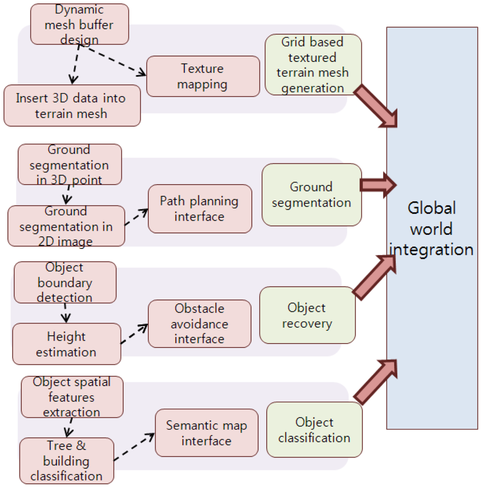
We describe a framework for outdoor terrain reconstruction and object classification, as shown in <xref ref-type="fig" rid="f1-sensors-12-11221">Figure 1</xref>. The integrated sensors provide a dataset of 2D images, 3D point clouds, and mobile robot navigation information. We integrate these dataset into a grid-based textured terrain mesh. Then, we describe a ground segmentation method that identifies the features such as the ground, obstacles, and the background.</p>
<p>As mentioned, for objects partially beyond the range of detection of the range sensor, we propose a height estimation method to recover the complete scene in the terrain mesh. Finally, we classify the objects into buildings and trees on the basis of their spatial distribution.</p>
<sec>
<label>3.1.</label>
<title>Grid-Based Textured Terrain Mesh</title>
<p>
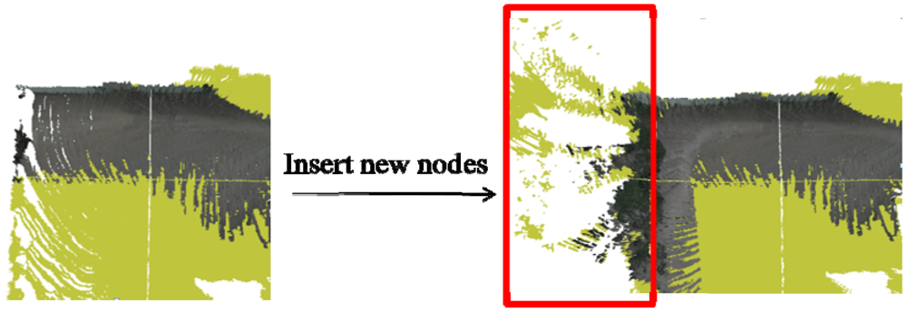
We integrate the sensed dataset into a grid-based textured terrain mesh. First, we project the 3D points onto the 2D image in front of the robot and get a coordinate in 2D image, named UV vector, for each 3D point. Then, we transform the local 3D points into global coordinates, and register them on the terrain mesh. The terrain mesh is generated using several grids, each with 151 × 151 textured vertices. In this application, the cell size is 0.125 × 0.125 m<sup>2</sup>. The height value of each cell is updated with the registered 3D points. If a new 3D point is to be inserted into the reconstructed terrain mesh but is outside the existing grids, we create a new grid to register this point, as shown in <xref ref-type="fig" rid="f2-sensors-12-11221">Figure 2</xref>.</p>
<p>After registration of all points, a ground segmentation algorithm is implemented to segment ground data and non-ground data in the 2D image. Then, a height estimation method is used to recover the missing regions outside the sensor's measurement range. Finally, the tree and building objects are classified using a classification operation. In our implementation, the user controls a virtual camera to study the reconstructed terrain from different viewpoints. A virtual robot model is loaded on the terrain to show the robot's navigation information in the real world.</p></sec>
<sec>
<label>3.2.</label>
<title>Ground Segmentation Method</title>
<p>We classify each pixel in the 2D image into ground and non-ground classes on the basis of the probability of it being in that configuration, which depends on its connected neighbors. Therefore, we can apply the MRF for ground segmentation. However, it is difficult to determine the probability because it must be computed from local and neighbor observations. According to the Hammersley-Clifford theorem, we can solve this problem using the Gibbs-MRF model.</p>
<p>Given observation <italic>d</italic> and configuration <italic>f</italic>, we find the best possible configuration <italic>f</italic>* for site <italic>s</italic> using the following optimum solution:
<disp-formula id="FD1">
<label>(1)</label>
<mml:math id="mm1" display="block">
<mml:semantics id="sm1">
<mml:mrow>
<mml:msup>
<mml:mi>f</mml:mi>
<mml:mo>∗</mml:mo></mml:msup>
<mml:mo stretchy="false">(</mml:mo>
<mml:mi>s</mml:mi>
<mml:mo stretchy="false">)</mml:mo>
<mml:mo>=</mml:mo>
<mml:mo>arg</mml:mo>
<mml:munder>
<mml:mrow>
<mml:mo>max</mml:mo></mml:mrow>
<mml:mi>f</mml:mi></mml:munder>
<mml:mi>p</mml:mi>
<mml:mo stretchy="false">(</mml:mo>
<mml:msub>
<mml:mi>X</mml:mi>
<mml:mi>s</mml:mi></mml:msub>
<mml:mo>=</mml:mo>
<mml:mi>f</mml:mi>
<mml:mo stretchy="false">|</mml:mo>
<mml:msub>
<mml:mi>X</mml:mi>
<mml:mi>t</mml:mi></mml:msub>
<mml:mo>=</mml:mo>
<mml:mi>d</mml:mi>
<mml:mo>,</mml:mo>
<mml:mo>∀</mml:mo>
<mml:mi>t</mml:mi>
<mml:mo>≠</mml:mo>
<mml:mi>s</mml:mi>
<mml:mo stretchy="false">)</mml:mo></mml:mrow></mml:semantics></mml:math></disp-formula></p>
<p>The probability of a site's configuration is calculated using the Gibbs distribution [<xref ref-type="bibr" rid="b22-sensors-12-11221">22</xref>]:
<disp-formula id="FD2">
<label>(2)</label>
<mml:math id="mm2" display="block">
<mml:semantics id="sm2">
<mml:mrow>
<mml:mi>p</mml:mi>
<mml:mo stretchy="false">(</mml:mo>
<mml:mi>f</mml:mi>
<mml:mo stretchy="false">)</mml:mo>
<mml:mo>=</mml:mo>
<mml:msup>
<mml:mi>Z</mml:mi>
<mml:mrow>
<mml:mo>−</mml:mo>
<mml:mn>1</mml:mn></mml:mrow></mml:msup>
<mml:msup>
<mml:mi>e</mml:mi>
<mml:mrow>
<mml:mo>−</mml:mo>
<mml:mfrac>
<mml:mn>1</mml:mn>
<mml:mi>T</mml:mi></mml:mfrac>
<mml:mi>U</mml:mi>
<mml:mo stretchy="false">(</mml:mo>
<mml:mi>f</mml:mi>
<mml:mo stretchy="false">)</mml:mo></mml:mrow></mml:msup></mml:mrow></mml:semantics></mml:math></disp-formula>
<disp-formula id="FD3">
<label>(3)</label>
<mml:math id="mm3" display="block">
<mml:semantics id="sm3">
<mml:mrow>
<mml:mi>U</mml:mi>
<mml:mo stretchy="false">(</mml:mo>
<mml:mi>f</mml:mi>
<mml:mo stretchy="false">)</mml:mo>
<mml:mo>=</mml:mo>
<mml:munder>
<mml:mo>∑</mml:mo>
<mml:mrow>
<mml:mi>c</mml:mi>
<mml:mo>∈</mml:mo>
<mml:mi>C</mml:mi></mml:mrow></mml:munder>
<mml:mrow>
<mml:msub>
<mml:mi>V</mml:mi>
<mml:mi>c</mml:mi></mml:msub>
<mml:mo stretchy="false">(</mml:mo>
<mml:mi>f</mml:mi>
<mml:mo stretchy="false">)</mml:mo></mml:mrow></mml:mrow></mml:semantics></mml:math></disp-formula>
<disp-formula id="FD4">
<label>(4)</label>
<mml:math id="mm4" display="block">
<mml:semantics id="sm4">
<mml:mrow>
<mml:mi>Z</mml:mi>
<mml:mo>=</mml:mo>
<mml:munder>
<mml:mo>∑</mml:mo>
<mml:mi>f</mml:mi></mml:munder>
<mml:mrow>
<mml:msup>
<mml:mi>e</mml:mi>
<mml:mrow>
<mml:mo>−</mml:mo>
<mml:mfrac>
<mml:mn>1</mml:mn>
<mml:mi>T</mml:mi></mml:mfrac>
<mml:mi>U</mml:mi>
<mml:mo stretchy="false">(</mml:mo>
<mml:mi>f</mml:mi>
<mml:mo stretchy="false">)</mml:mo></mml:mrow></mml:msup></mml:mrow></mml:mrow></mml:semantics></mml:math></disp-formula></p>
<p>We define a clique as a neighboring set, and a clique set <italic>C</italic> as a collection of single-site and pair-site cliques. A potential function <italic>V<sub>c</sub></italic>(<italic>f</italic>) is defined to evaluate the effect of neighbor sites in clique <italic>c</italic>.</p>
<p>According to the Bayes' rule, the solution of <xref rid="FD1" ref-type="disp-formula">Equation (1)</xref> is as follows:
<disp-formula id="FD5">
<label>(5)</label>
<mml:math id="mm5" display="block">
<mml:semantics id="sm5">
<mml:mrow>
<mml:msup>
<mml:mi>f</mml:mi>
<mml:mo>∗</mml:mo></mml:msup>
<mml:mo>=</mml:mo>
<mml:mo>arg</mml:mo>
<mml:munder>
<mml:mrow>
<mml:mo>max</mml:mo></mml:mrow>
<mml:mi>f</mml:mi></mml:munder>
<mml:mi>p</mml:mi>
<mml:mo stretchy="false">(</mml:mo>
<mml:mi>f</mml:mi>
<mml:mo stretchy="false">|</mml:mo>
<mml:mi>d</mml:mi>
<mml:mo stretchy="false">)</mml:mo>
<mml:mo>=</mml:mo>
<mml:mo>arg</mml:mo>
<mml:munder>
<mml:mrow>
<mml:mo>max</mml:mo></mml:mrow>
<mml:mi>f</mml:mi></mml:munder>
<mml:mi>p</mml:mi>
<mml:mo stretchy="false">(</mml:mo>
<mml:mi>d</mml:mi>
<mml:mo stretchy="false">|</mml:mo>
<mml:mi>f</mml:mi>
<mml:mo stretchy="false">)</mml:mo>
<mml:mi>p</mml:mi>
<mml:mo stretchy="false">(</mml:mo>
<mml:mi>f</mml:mi>
<mml:mo stretchy="false">)</mml:mo>
<mml:mo>=</mml:mo>
<mml:mo>arg</mml:mo>
<mml:munder>
<mml:mrow>
<mml:mo>min</mml:mo></mml:mrow>
<mml:mi>f</mml:mi></mml:munder>
<mml:mi>U</mml:mi>
<mml:mo stretchy="false">(</mml:mo>
<mml:mi>f</mml:mi>
<mml:mo stretchy="false">|</mml:mo>
<mml:mi>d</mml:mi>
<mml:mo stretchy="false">)</mml:mo>
<mml:mo>=</mml:mo>
<mml:mo>arg</mml:mo>
<mml:munder>
<mml:mrow>
<mml:mo>min</mml:mo></mml:mrow>
<mml:mi>f</mml:mi></mml:munder>
<mml:mo stretchy="false">{</mml:mo>
<mml:mi>U</mml:mi>
<mml:mo stretchy="false">(</mml:mo>
<mml:mi>d</mml:mi>
<mml:mo stretchy="false">|</mml:mo>
<mml:mi>f</mml:mi>
<mml:mo stretchy="false">)</mml:mo>
<mml:mo>+</mml:mo>
<mml:mi>U</mml:mi>
<mml:mo stretchy="false">(</mml:mo>
<mml:mi>f</mml:mi>
<mml:mo stretchy="false">)</mml:mo>
<mml:mo stretchy="false">}</mml:mo></mml:mrow></mml:semantics></mml:math></disp-formula></p>
<p>The energy function of <italic>U</italic>(<italic>d</italic>|<italic>f</italic>) + <italic>U</italic>(<italic>f</italic>) is defined to evaluate the effect of the neighbor sites in single-site and pair-site potential cliques, as follows:
<disp-formula id="FD6">
<label>(6)</label>
<mml:math id="mm6" display="block">
<mml:semantics id="sm6">
<mml:mrow>
<mml:mi>U</mml:mi>
<mml:mo stretchy="false">(</mml:mo>
<mml:mi>d</mml:mi>
<mml:mo stretchy="false">|</mml:mo>
<mml:mi>f</mml:mi>
<mml:mo stretchy="false">)</mml:mo>
<mml:mo>+</mml:mo>
<mml:mi>U</mml:mi>
<mml:mo stretchy="false">(</mml:mo>
<mml:mi>f</mml:mi>
<mml:mo stretchy="false">)</mml:mo>
<mml:mo>=</mml:mo>
<mml:munder>
<mml:mo>∑</mml:mo>
<mml:mrow>
<mml:mi>s</mml:mi>
<mml:mo>∈</mml:mo>
<mml:msub>
<mml:mi>C</mml:mi>
<mml:mn>1</mml:mn></mml:msub></mml:mrow></mml:munder>
<mml:mrow>
<mml:msub>
<mml:mi>V</mml:mi>
<mml:mn>1</mml:mn></mml:msub>
<mml:mo stretchy="false">(</mml:mo>
<mml:msub>
<mml:mi>f</mml:mi>
<mml:mi>s</mml:mi></mml:msub>
<mml:mo stretchy="false">)</mml:mo></mml:mrow>
<mml:mo>+</mml:mo>
<mml:munder>
<mml:mo>∑</mml:mo>
<mml:mrow>
<mml:mo stretchy="false">{</mml:mo>
<mml:mi>s</mml:mi>
<mml:mo>,</mml:mo>
<mml:mi>s</mml:mi>
<mml:mo>'</mml:mo>
<mml:mo stretchy="false">}</mml:mo>
<mml:mo>∈</mml:mo>
<mml:msub>
<mml:mi>C</mml:mi>
<mml:mn>2</mml:mn></mml:msub></mml:mrow></mml:munder>
<mml:mrow>
<mml:msub>
<mml:mi>V</mml:mi>
<mml:mn>2</mml:mn></mml:msub>
<mml:mo stretchy="false">(</mml:mo>
<mml:msub>
<mml:mi>f</mml:mi>
<mml:mi>s</mml:mi></mml:msub>
<mml:mo>,</mml:mo>
<mml:msub>
<mml:mi>f</mml:mi>
<mml:mrow>
<mml:mi>s</mml:mi>
<mml:mo>'</mml:mo></mml:mrow></mml:msub>
<mml:mo stretchy="false">)</mml:mo></mml:mrow>
<mml:mo>+</mml:mo>
<mml:munder>
<mml:mo>∑</mml:mo>
<mml:mrow>
<mml:mi>s</mml:mi>
<mml:mo>∈</mml:mo>
<mml:msub>
<mml:mi>C</mml:mi>
<mml:mn>1</mml:mn></mml:msub></mml:mrow></mml:munder>
<mml:mrow>
<mml:msub>
<mml:mi>V</mml:mi>
<mml:mn>1</mml:mn></mml:msub>
<mml:mo stretchy="false">(</mml:mo>
<mml:msub>
<mml:mi>d</mml:mi>
<mml:mi>s</mml:mi></mml:msub>
<mml:mo stretchy="false">|</mml:mo>
<mml:msub>
<mml:mi>f</mml:mi>
<mml:mi>s</mml:mi></mml:msub>
<mml:mo stretchy="false">)</mml:mo></mml:mrow>
<mml:mo>+</mml:mo>
<mml:munder>
<mml:mo>∑</mml:mo>
<mml:mrow>
<mml:mo stretchy="false">{</mml:mo>
<mml:mi>s</mml:mi>
<mml:mo>,</mml:mo>
<mml:mi>s</mml:mi>
<mml:mo>'</mml:mo>
<mml:mo stretchy="false">}</mml:mo>
<mml:mo>∈</mml:mo>
<mml:msub>
<mml:mi>C</mml:mi>
<mml:mn>2</mml:mn></mml:msub></mml:mrow></mml:munder>
<mml:mrow>
<mml:msub>
<mml:mi>V</mml:mi>
<mml:mn>2</mml:mn></mml:msub>
<mml:mo stretchy="false">(</mml:mo>
<mml:msub>
<mml:mi>d</mml:mi>
<mml:mi>s</mml:mi></mml:msub>
<mml:mo>,</mml:mo>
<mml:msub>
<mml:mi>d</mml:mi>
<mml:mrow>
<mml:mi>s</mml:mi>
<mml:mo>'</mml:mo></mml:mrow></mml:msub>
<mml:mo stretchy="false">|</mml:mo>
<mml:msub>
<mml:mi>f</mml:mi>
<mml:mi>s</mml:mi></mml:msub>
<mml:mo>,</mml:mo>
<mml:msub>
<mml:mi>f</mml:mi>
<mml:mrow>
<mml:mi>s</mml:mi>
<mml:mo>'</mml:mo></mml:mrow></mml:msub>
<mml:mo stretchy="false">)</mml:mo></mml:mrow></mml:mrow></mml:semantics></mml:math></disp-formula></p>
<p>The evaluations of the clique potential functions <italic>V</italic><sub>1</sub>(<italic>f<sub>s</sub></italic>) and <italic>V</italic><sub>1</sub>(<italic>d<sub>s</sub></italic>|<italic>f<sub>s</sub></italic>) depend on the local configuration and observations of clique <italic>C</italic><sub>1</sub>. The clique potential functions <italic>V</italic><sub>2</sub>(<italic>f<sub>s</sub></italic>, <italic>f<sub>s'</sub></italic>) and <italic>V</italic><sub>2</sub>(<italic>d<sub>s</sub></italic>, <italic>d<sub>s'</sub></italic>|<italic>f<sub>s</sub></italic>, <italic>f<sub>s'</sub></italic>) are evaluations of the pair-site consistency of clique <italic>C</italic><sub>2</sub>.</p>
<p>
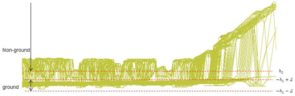
When we apply the Gibbs-MRF to ground segmentation in a 2D image, we first determine a set of pixels whose configurations are in the ground class with high confidence. We initially segment the 3D points as ground data using the robot vehicle's height <italic>h</italic><sub>1</sub> as the standard. We assume that if the y coordinate of a 3D point is ranging from −<italic>h</italic><sub>1</sub> − Δ to −<italic>h</italic><sub>1</sub> + Δ, then this point is ground data, as shown in <xref ref-type="fig" rid="f3-sensors-12-11221">Figure 3</xref>. This step is a rough ground segmentation process, which produces a dataset <italic>G</italic><sub>1</sub>.</p>
<p>Then we find the projected pixels in the 2D image from the points in <italic>G</italic><sub>1</sub>, using the projection matrix as follows:
<disp-formula id="FD7">
<label>(7)</label>
<mml:math id="mm7" display="block">
<mml:semantics id="sm7">
<mml:mrow>
<mml:mi>t</mml:mi>
<mml:mo>=</mml:mo>
<mml:mi>K</mml:mi>
<mml:mi>R</mml:mi>
<mml:mo stretchy="false">[</mml:mo>
<mml:mi>I</mml:mi>
<mml:mo stretchy="false">|</mml:mo>
<mml:mo>−</mml:mo>
<mml:mtext mathvariant="italic">Cam</mml:mtext>
<mml:mo stretchy="false">]</mml:mo>
<mml:mi>T</mml:mi></mml:mrow></mml:semantics></mml:math></disp-formula>where the homogeneous coordinates of image pixel <italic>t</italic> are projected from the homogeneous coordinates of the 3D point <italic>T</italic>. Cam is defined as the vector of the camera's position, the matrix <italic>R</italic> is defined as the mobile rotation matrix, and <italic>I</italic> is an identity matrix. The camera calibration matrix <italic>K</italic> is defined as follows:
<disp-formula id="FD8">
<label>(8)</label>
<mml:math id="mm8" display="block">
<mml:semantics id="sm8">
<mml:mrow>
<mml:mi>K</mml:mi>
<mml:mo>=</mml:mo>
<mml:mrow>
<mml:mo>[</mml:mo>
<mml:mrow>
<mml:mtable>
<mml:mtr>
<mml:mtd>
<mml:mi>l</mml:mi></mml:mtd>
<mml:mtd>
<mml:mn>0</mml:mn></mml:mtd>
<mml:mtd>
<mml:mrow>
<mml:msub>
<mml:mi>p</mml:mi>
<mml:mi>x</mml:mi></mml:msub></mml:mrow></mml:mtd></mml:mtr>
<mml:mtr>
<mml:mtd>
<mml:mn>0</mml:mn></mml:mtd>
<mml:mtd>
<mml:mi>l</mml:mi></mml:mtd>
<mml:mtd>
<mml:mrow>
<mml:msub>
<mml:mi>p</mml:mi>
<mml:mi>y</mml:mi></mml:msub></mml:mrow></mml:mtd></mml:mtr>
<mml:mtr>
<mml:mtd>
<mml:mn>0</mml:mn></mml:mtd>
<mml:mtd>
<mml:mn>0</mml:mn></mml:mtd>
<mml:mtd>
<mml:mn>1</mml:mn></mml:mtd></mml:mtr></mml:mtable></mml:mrow>
<mml:mo>]</mml:mo></mml:mrow></mml:mrow></mml:semantics></mml:math></disp-formula>where <italic>l</italic> is the focal length of the camera, and the 2D coordinate (<italic>p<sub>x</sub></italic>, <italic>p<sub>y</sub></italic>) is the center position of the captured image. As shown in <xref ref-type="fig" rid="f4-sensors-12-11221">Figure 4</xref>, the 2D pixel dataset 
<inline-formula>
<mml:math id="mm9" display="inline">
<mml:semantics id="sm9">
<mml:mrow>
<mml:msubsup>
<mml:mi>G</mml:mi>
<mml:mn>1</mml:mn>
<mml:mo>'</mml:mo></mml:msubsup></mml:mrow></mml:semantics></mml:math></inline-formula> is mapped from the dataset <italic>G</italic><sub>1</sub>. We determine the configuration of site 
<inline-formula>
<mml:math id="mm10" display="inline">
<mml:semantics id="sm10">
<mml:mrow>
<mml:mi>s</mml:mi>
<mml:mo>∈</mml:mo>
<mml:msubsup>
<mml:mi>G</mml:mi>
<mml:mn>1</mml:mn>
<mml:mo>'</mml:mo></mml:msubsup></mml:mrow></mml:semantics></mml:math></inline-formula> as ground.</p>
<p>We apply the Gibbs-MRF algorithm to classify the configurations of other pixels into the ground or non-ground classes. We consider that:
<list list-type="alpha-lower">
<list-item>
<p>If the configuration of site <italic>s</italic> is same as its observation, the probability of this configuration is high.</p></list-item>
<list-item>
<p>If the configuration of site <italic>s</italic> is same as the configuration of its neighboring site <italic>s'</italic>, the probability of this configuration is high.</p></list-item>
<list-item>
<p>If the configuration of site <italic>s</italic> is same as the configuration of its neighboring site <italic>s'</italic>, and the difference between these observations <italic>d<sub>s</sub></italic> and <italic>d<sub>s</sub></italic><sub>′</sub> is low, the probability of this configuration is high.</p></list-item></list></p>
<p>The clique potential functions are formulated as follows:
<disp-formula id="FD9">
<label>(9)</label>
<mml:math id="mm11" display="block">
<mml:semantics id="sm11">
<mml:mrow>
<mml:msub>
<mml:mi>V</mml:mi>
<mml:mn>1</mml:mn></mml:msub>
<mml:mo stretchy="false">(</mml:mo>
<mml:msub>
<mml:mi>f</mml:mi>
<mml:mi>s</mml:mi></mml:msub>
<mml:mo stretchy="false">)</mml:mo>
<mml:mo>=</mml:mo>
<mml:mrow>
<mml:mo stretchy="true">{</mml:mo>
<mml:mrow>
<mml:mtable>
<mml:mtr>
<mml:mtd>
<mml:mrow>
<mml:mo>−</mml:mo>
<mml:mi>α</mml:mi></mml:mrow></mml:mtd>
<mml:mtd>
<mml:mrow>
<mml:mi>i</mml:mi>
<mml:mi>f</mml:mi>
<mml:mo stretchy="false">(</mml:mo>
<mml:mi>s</mml:mi>
<mml:mo>∈</mml:mo>
<mml:msub>
<mml:mi>G</mml:mi>
<mml:mn>1</mml:mn></mml:msub></mml:mrow></mml:mtd>
<mml:mtd>
<mml:mrow>
<mml:mtext mathvariant="italic">and</mml:mtext></mml:mrow></mml:mtd>
<mml:mtd>
<mml:mrow>
<mml:msub>
<mml:mi>f</mml:mi>
<mml:mi>s</mml:mi></mml:msub>
<mml:mo>=</mml:mo>
<mml:mtext mathvariant="italic">ground</mml:mtext>
<mml:mo stretchy="false">)</mml:mo></mml:mrow></mml:mtd></mml:mtr>
<mml:mtr>
<mml:mtd/>
<mml:mtd>
<mml:mrow>
<mml:mi>o</mml:mi>
<mml:mi>r</mml:mi>
<mml:mo stretchy="false">(</mml:mo>
<mml:mi>s</mml:mi>
<mml:mo>∉</mml:mo>
<mml:msub>
<mml:mi>G</mml:mi>
<mml:mn>1</mml:mn></mml:msub></mml:mrow></mml:mtd>
<mml:mtd>
<mml:mrow>
<mml:mtext mathvariant="italic">and</mml:mtext></mml:mrow></mml:mtd>
<mml:mtd>
<mml:mrow>
<mml:msub>
<mml:mi>f</mml:mi>
<mml:mi>s</mml:mi></mml:msub>
<mml:mo>=</mml:mo>
<mml:mtext mathvariant="italic">nonground</mml:mtext>
<mml:mo stretchy="false">)</mml:mo></mml:mrow></mml:mtd></mml:mtr>
<mml:mtr>
<mml:mtd>
<mml:mrow>
<mml:mo>+</mml:mo>
<mml:mi>α</mml:mi></mml:mrow></mml:mtd>
<mml:mtd>
<mml:mrow>
<mml:mi>i</mml:mi>
<mml:mi>f</mml:mi>
<mml:mo stretchy="false">(</mml:mo>
<mml:mi>s</mml:mi>
<mml:mo>∉</mml:mo>
<mml:msub>
<mml:mi>G</mml:mi>
<mml:mn>1</mml:mn></mml:msub></mml:mrow></mml:mtd>
<mml:mtd>
<mml:mrow>
<mml:mtext mathvariant="italic">and</mml:mtext></mml:mrow></mml:mtd>
<mml:mtd>
<mml:mrow>
<mml:msub>
<mml:mi>f</mml:mi>
<mml:mi>s</mml:mi></mml:msub>
<mml:mo>=</mml:mo>
<mml:mtext mathvariant="italic">ground</mml:mtext>
<mml:mo stretchy="false">)</mml:mo></mml:mrow></mml:mtd></mml:mtr>
<mml:mtr>
<mml:mtd/>
<mml:mtd>
<mml:mrow>
<mml:mi>o</mml:mi>
<mml:mi>r</mml:mi>
<mml:mo stretchy="false">(</mml:mo>
<mml:mi>s</mml:mi>
<mml:mo>∈</mml:mo>
<mml:msub>
<mml:mi>G</mml:mi>
<mml:mn>1</mml:mn></mml:msub></mml:mrow></mml:mtd>
<mml:mtd>
<mml:mrow>
<mml:mtext mathvariant="italic">and</mml:mtext></mml:mrow></mml:mtd>
<mml:mtd>
<mml:mrow>
<mml:msub>
<mml:mi>f</mml:mi>
<mml:mi>s</mml:mi></mml:msub>
<mml:mo>=</mml:mo>
<mml:mtext mathvariant="italic">nonground</mml:mtext>
<mml:mo stretchy="false">)</mml:mo></mml:mrow></mml:mtd></mml:mtr></mml:mtable></mml:mrow></mml:mrow></mml:mrow></mml:semantics></mml:math></disp-formula>
<disp-formula id="FD10">
<label>(10)</label>
<mml:math id="mm12" display="block">
<mml:semantics id="sm12">
<mml:mrow>
<mml:msub>
<mml:mi>V</mml:mi>
<mml:mn>1</mml:mn></mml:msub>
<mml:mo stretchy="false">(</mml:mo>
<mml:msub>
<mml:mi>d</mml:mi>
<mml:mi>s</mml:mi></mml:msub>
<mml:mo stretchy="false">|</mml:mo>
<mml:msub>
<mml:mi>f</mml:mi>
<mml:mi>s</mml:mi></mml:msub>
<mml:mo stretchy="false">)</mml:mo>
<mml:mo>=</mml:mo>
<mml:mrow>
<mml:mo stretchy="true">{</mml:mo>
<mml:mrow>
<mml:mtable>
<mml:mtr>
<mml:mtd>
<mml:mrow>
<mml:mo>−</mml:mo>
<mml:mi>α</mml:mi></mml:mrow></mml:mtd>
<mml:mtd>
<mml:mrow>
<mml:mi>i</mml:mi>
<mml:mi>f</mml:mi>
<mml:mo stretchy="false">(</mml:mo>
<mml:msub>
<mml:mi>d</mml:mi>
<mml:mi>s</mml:mi></mml:msub>
<mml:mo>=</mml:mo>
<mml:msub>
<mml:mi>f</mml:mi>
<mml:mi>s</mml:mi></mml:msub>
<mml:mo stretchy="false">)</mml:mo></mml:mrow></mml:mtd></mml:mtr>
<mml:mtr>
<mml:mtd>
<mml:mrow>
<mml:mo>+</mml:mo>
<mml:mi>α</mml:mi></mml:mrow></mml:mtd>
<mml:mtd>
<mml:mrow>
<mml:mi>i</mml:mi>
<mml:mi>f</mml:mi>
<mml:mo stretchy="false">(</mml:mo>
<mml:msub>
<mml:mi>d</mml:mi>
<mml:mi>s</mml:mi></mml:msub>
<mml:mo>≠</mml:mo>
<mml:msub>
<mml:mi>f</mml:mi>
<mml:mi>s</mml:mi></mml:msub>
<mml:mo stretchy="false">)</mml:mo></mml:mrow></mml:mtd></mml:mtr></mml:mtable></mml:mrow></mml:mrow></mml:mrow></mml:semantics></mml:math></disp-formula>
<disp-formula id="FD11">
<label>(11)</label>
<mml:math id="mm13" display="block">
<mml:semantics id="sm13">
<mml:mrow>
<mml:msub>
<mml:mi>V</mml:mi>
<mml:mn>1</mml:mn></mml:msub>
<mml:mo stretchy="false">(</mml:mo>
<mml:msub>
<mml:mi>f</mml:mi>
<mml:mi>s</mml:mi></mml:msub>
<mml:mo>,</mml:mo>
<mml:msub>
<mml:mi>f</mml:mi>
<mml:mrow>
<mml:mi>s</mml:mi>
<mml:mo>'</mml:mo></mml:mrow></mml:msub>
<mml:mo stretchy="false">)</mml:mo>
<mml:mo>=</mml:mo>
<mml:mrow>
<mml:mo stretchy="true">{</mml:mo>
<mml:mrow>
<mml:mtable>
<mml:mtr>
<mml:mtd>
<mml:mrow>
<mml:mo>−</mml:mo>
<mml:mi>β</mml:mi></mml:mrow></mml:mtd>
<mml:mtd>
<mml:mrow>
<mml:mi>i</mml:mi>
<mml:mi>f</mml:mi>
<mml:mo stretchy="false">(</mml:mo>
<mml:msub>
<mml:mi>f</mml:mi>
<mml:mi>s</mml:mi></mml:msub>
<mml:mo>=</mml:mo>
<mml:msub>
<mml:mi>f</mml:mi>
<mml:mi>s</mml:mi></mml:msub>
<mml:mo stretchy="false">)</mml:mo></mml:mrow></mml:mtd></mml:mtr>
<mml:mtr>
<mml:mtd>
<mml:mrow>
<mml:mo>+</mml:mo>
<mml:mi>β</mml:mi></mml:mrow></mml:mtd>
<mml:mtd>
<mml:mrow>
<mml:mi>i</mml:mi>
<mml:mi>f</mml:mi>
<mml:mo stretchy="false">(</mml:mo>
<mml:msub>
<mml:mi>f</mml:mi>
<mml:mi>s</mml:mi></mml:msub>
<mml:mo>≠</mml:mo>
<mml:msub>
<mml:mi>f</mml:mi>
<mml:mi>s</mml:mi></mml:msub>
<mml:mo stretchy="false">)</mml:mo></mml:mrow></mml:mtd></mml:mtr></mml:mtable></mml:mrow></mml:mrow></mml:mrow></mml:semantics></mml:math></disp-formula>
<disp-formula id="FD12">
<label>(12)</label>
<mml:math id="mm14" display="block">
<mml:semantics id="sm14">
<mml:mrow>
<mml:msub>
<mml:mi>V</mml:mi>
<mml:mn>1</mml:mn></mml:msub>
<mml:mo stretchy="false">(</mml:mo>
<mml:msub>
<mml:mi>d</mml:mi>
<mml:mi>s</mml:mi></mml:msub>
<mml:mo>,</mml:mo>
<mml:msub>
<mml:mi>d</mml:mi>
<mml:mrow>
<mml:mi>s</mml:mi>
<mml:mo>'</mml:mo></mml:mrow></mml:msub>
<mml:mo stretchy="false">|</mml:mo>
<mml:msub>
<mml:mi>f</mml:mi>
<mml:mi>s</mml:mi></mml:msub>
<mml:mo>,</mml:mo>
<mml:msub>
<mml:mi>f</mml:mi>
<mml:mrow>
<mml:mi>s</mml:mi>
<mml:mo>'</mml:mo></mml:mrow></mml:msub>
<mml:mo stretchy="false">)</mml:mo>
<mml:mo>=</mml:mo>
<mml:mrow>
<mml:mo stretchy="true">{</mml:mo>
<mml:mrow>
<mml:mtable>
<mml:mtr>
<mml:mtd>
<mml:mrow>
<mml:mo>−</mml:mo>
<mml:mi>γ</mml:mi>
<mml:msup>
<mml:mi>e</mml:mi>
<mml:mrow>
<mml:mo>−</mml:mo>
<mml:mo stretchy="false">‖</mml:mo>
<mml:msub>
<mml:mi>d</mml:mi>
<mml:mi>s</mml:mi></mml:msub>
<mml:mo>−</mml:mo>
<mml:msub>
<mml:mi>d</mml:mi>
<mml:mrow>
<mml:mi>s</mml:mi>
<mml:mo>'</mml:mo></mml:mrow></mml:msub>
<mml:mo stretchy="false">‖</mml:mo></mml:mrow></mml:msup></mml:mrow></mml:mtd>
<mml:mtd>
<mml:mrow>
<mml:mi>i</mml:mi>
<mml:mi>f</mml:mi>
<mml:mo stretchy="false">(</mml:mo>
<mml:msub>
<mml:mi>f</mml:mi>
<mml:mi>s</mml:mi></mml:msub>
<mml:mo>=</mml:mo>
<mml:msub>
<mml:mi>f</mml:mi>
<mml:mrow>
<mml:mi>s</mml:mi>
<mml:mo>'</mml:mo></mml:mrow></mml:msub>
<mml:mo stretchy="false">)</mml:mo></mml:mrow></mml:mtd></mml:mtr>
<mml:mtr>
<mml:mtd>
<mml:mrow>
<mml:mo>+</mml:mo>
<mml:mi>γ</mml:mi>
<mml:msup>
<mml:mi>e</mml:mi>
<mml:mrow>
<mml:mo>−</mml:mo>
<mml:mo stretchy="false">‖</mml:mo>
<mml:msub>
<mml:mi>d</mml:mi>
<mml:mi>s</mml:mi></mml:msub>
<mml:mo>−</mml:mo>
<mml:msub>
<mml:mi>d</mml:mi>
<mml:mrow>
<mml:mi>s</mml:mi>
<mml:mo>'</mml:mo></mml:mrow></mml:msub>
<mml:mo stretchy="false">‖</mml:mo></mml:mrow></mml:msup></mml:mrow></mml:mtd>
<mml:mtd>
<mml:mrow>
<mml:mi>i</mml:mi>
<mml:mi>f</mml:mi>
<mml:mo stretchy="false">(</mml:mo>
<mml:msub>
<mml:mi>f</mml:mi>
<mml:mi>s</mml:mi></mml:msub>
<mml:mo>≠</mml:mo>
<mml:msub>
<mml:mi>f</mml:mi>
<mml:mrow>
<mml:mi>s</mml:mi>
<mml:mo>'</mml:mo></mml:mrow></mml:msub>
<mml:mo stretchy="false">)</mml:mo></mml:mrow></mml:mtd></mml:mtr></mml:mtable></mml:mrow></mml:mrow></mml:mrow></mml:semantics></mml:math></disp-formula></p>
<p>Here, the constants <italic>α</italic>, <italic>β</italic>, and <italic>γ</italic> are positive numerical values. The configuration <italic>f<sub>s</sub></italic> depends on whether the pixel <italic>s</italic> belongs to the ground dataset 
<inline-formula>
<mml:math id="mm15" display="inline">
<mml:semantics id="sm15">
<mml:mrow>
<mml:msubsup>
<mml:mi>G</mml:mi>
<mml:mn>1</mml:mn>
<mml:mo>'</mml:mo></mml:msubsup></mml:mrow></mml:semantics></mml:math></inline-formula>. The formula ‖<italic>d<sub>s</sub></italic> – <italic>d<sub>s'</sub></italic>‖ is defined as the color difference between observations <italic>d<sub>s</sub></italic> and <italic>d<sub>s'</sub></italic>.</p>
<p>We derive <xref rid="FD5" ref-type="disp-formula">Equation (5)</xref> using the potential functions defined in Equations (9–12), and label the configuration of each pixel.</p>
<p>To reduce the computation load of Gibbs-MRF, we apply a flood-fill algorithm to compute the configurations of pixels inside the boundary between ground and non-ground. The pseudocode for ground segmentation using the flood-fill algorithm is as follows:
<array>
<tbody>
<tr>
<td align="left" valign="top">for each site <italic>s</italic> in 
<inline-formula>
<mml:math id="mm16" display="inline">
<mml:semantics id="sm16">
<mml:mrow>
<mml:msubsup>
<mml:mi>G</mml:mi>
<mml:mn>1</mml:mn>
<mml:mo>'</mml:mo></mml:msubsup></mml:mrow></mml:semantics></mml:math></inline-formula></td></tr>
<tr>
<td align="left" valign="top"> configuration <italic>f</italic>(<italic>s</italic>) = ground;</td></tr>
<tr>
<td align="left" valign="top"> enqueue neighbour sites of <italic>s</italic> into a queue Q;</td></tr>
<tr>
<td align="left" valign="top"> while (Q is not empty)</td></tr>
<tr>
<td align="left" valign="top">  dequeue a site <italic>s′</italic> from the Q;</td></tr>
<tr>
<td align="left" valign="top">  if (<italic>f</italic>* (<italic>s</italic>′) =ground)</td></tr>
<tr>
<td align="left" valign="top">   enqueue neighbor sites of <italic>s′</italic> into Q;</td></tr>
<tr>
<td align="left" valign="top">  endif;</td></tr>
<tr>
<td align="left" valign="top"> endwhile;</td></tr>
<tr>
<td align="left" valign="top">endfor;</td></tr></tbody></array></p>
<p>Starting with the pixel set 
<inline-formula>
<mml:math id="mm17" display="inline">
<mml:semantics id="sm17">
<mml:mrow>
<mml:msubsup>
<mml:mi>G</mml:mi>
<mml:mn>1</mml:mn>
<mml:mo>'</mml:mo></mml:msubsup></mml:mrow></mml:semantics></mml:math></inline-formula>, we estimate the configurations of the neighboring pixels. We apply the Gibbs-MRF algorithm to classify the configurations of other pixels into the ground or non-ground classes.</p>
<p>The pixels with a ground configuration are grouped into dataset 
<inline-formula>
<mml:math id="mm18" display="inline">
<mml:semantics id="sm18">
<mml:mrow>
<mml:msubsup>
<mml:mi>G</mml:mi>
<mml:mn>2</mml:mn>
<mml:mo>'</mml:mo></mml:msubsup></mml:mrow></mml:semantics></mml:math></inline-formula>, which is shown as the blue region. The other regions contain objects and background textures. We classify the ground vertices in the 3D terrain mesh, which are mapped to the pixels in the dataset 
<inline-formula>
<mml:math id="mm19" display="inline">
<mml:semantics id="sm19">
<mml:mrow>
<mml:msubsup>
<mml:mi>G</mml:mi>
<mml:mn>2</mml:mn>
<mml:mo>'</mml:mo></mml:msubsup></mml:mrow></mml:semantics></mml:math></inline-formula>, as shown in <xref ref-type="fig" rid="f11-sensors-12-11221">Figure 11(b)</xref>.</p></sec>
<sec>
<label>3.3.</label>
<title>Complete Scene Recovery</title>
<p>
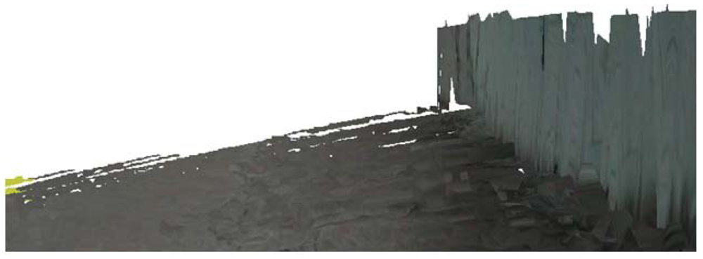
When mobile robots detect surrounding terrain information, some parts of objects are outside the measurement of range sensors. We see that the top of the building is missing in the terrain reconstruction result, shown as <xref ref-type="fig" rid="f5-sensors-12-11221">Figure 5</xref>.</p>
<p>We propose a height estimation method to solve the problem of missing regions by estimating the y coordinate of an object's top boundary.</p>
<p>
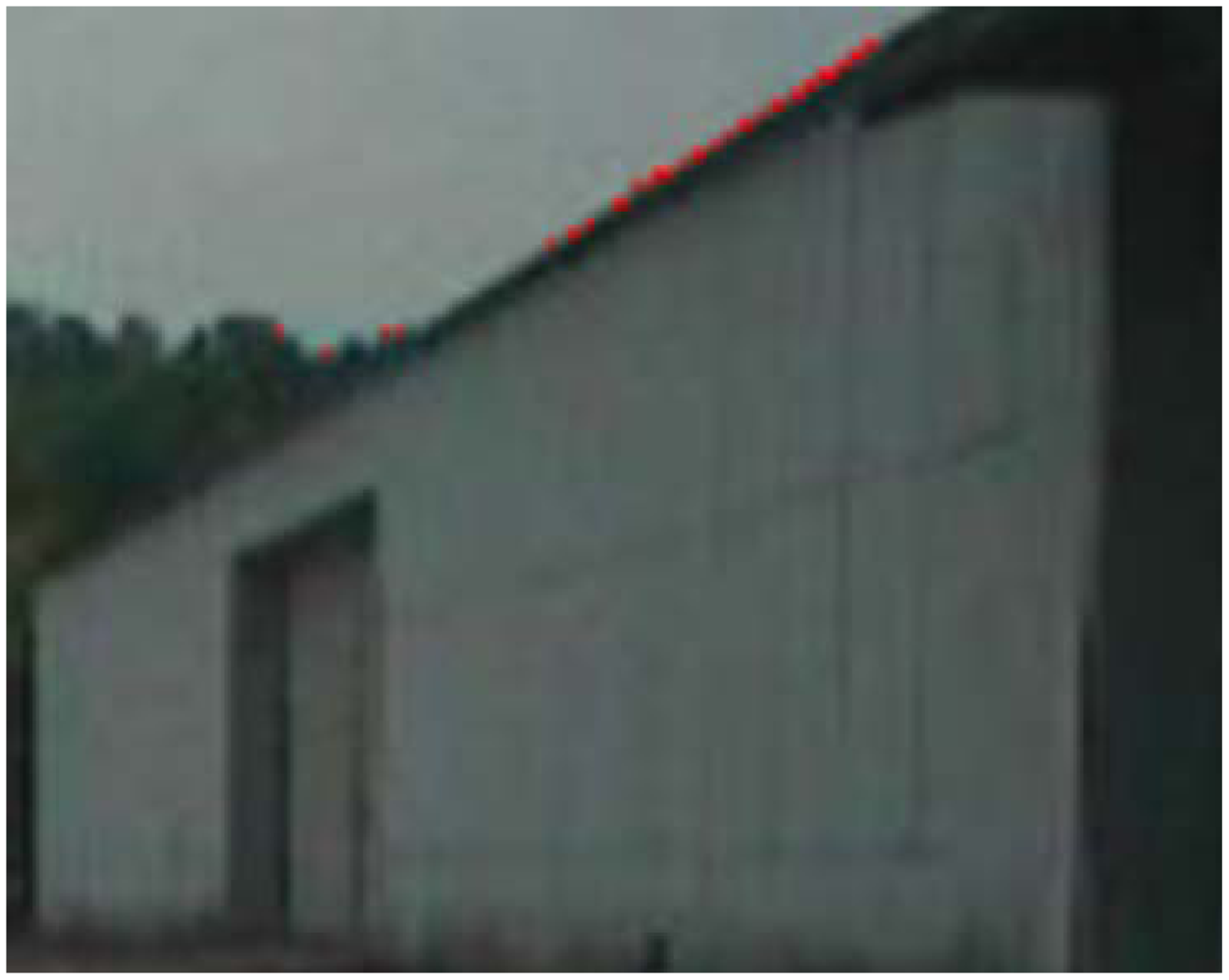
Using the ground data segmentation result, we assume that the non-ground vertices in the terrain mesh belong to objects, because background data, such as the sky, cannot be sensed by the range sensor. Next, we project these vertices onto pixels in a 2D image, whose configuration is determined as being part of an object. We apply the Gibbs-MRF method to classify the non-ground pixels into objects and background classes, in order to detect the boundary pixels between objects and background. The boundary detection results are shown as red pixels in <xref ref-type="fig" rid="f6-sensors-12-11221">Figure 6</xref>.</p>
<p>
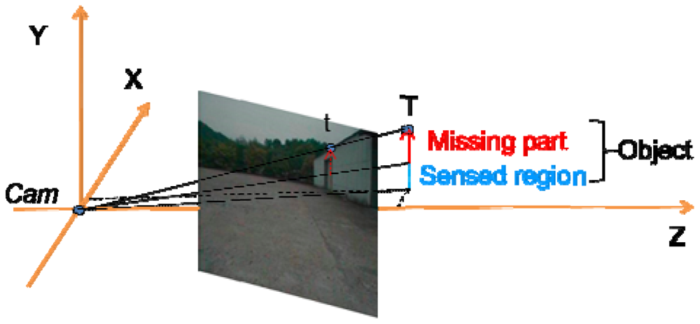
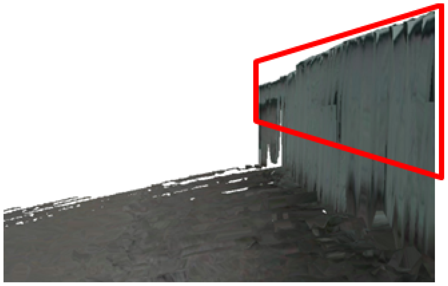
We find the boundary's y coordinates using an inverse process of projection from 2D pixels to 3D points. We place the camera centre at the origin. The projection ray from the origin to the object vertex gives an estimate of the height of that object vertex, as shown in <xref ref-type="fig" rid="f7-sensors-12-11221">Figure 7</xref>. Because the horizon coordinates of the 3D object vertex in the terrain mesh are fixed, we update the elevation value of each object vertex in the terrain mesh to obtain the results shown in <xref ref-type="fig" rid="f8-sensors-12-11221">Figure 8</xref>.</p></sec>
<sec>
<label>3.4.</label>
<title>Building and Tree Classification</title>
<p>
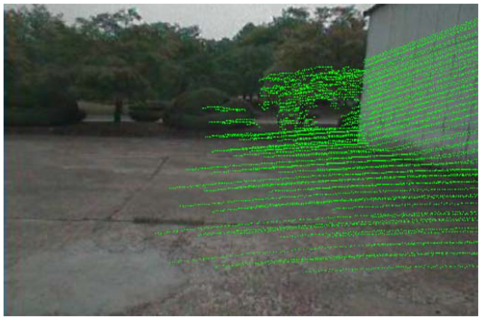
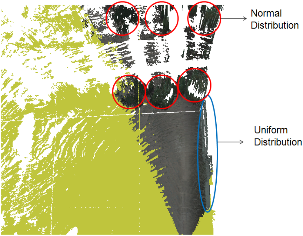
We consider tree objects, including both grass and trees, to have a porous surface that allows rays from the range finder to pierce through to the inside. This is in contrast to buildings, for which the 3D range finder only detects points on the outer surface. Therefore, the horizon shape of a building has a uniform distribution, whereas that for a tree has a normal distribution. As shown in <xref ref-type="fig" rid="f9-sensors-12-11221">Figure 9</xref>, we can see that the horizon structure of the buildings consists of the line-like components. We classify buildings by detecting these lines using the masks described in <xref ref-type="fig" rid="f10-sensors-12-11221">Figure 10</xref>.</p>
<p>The convolution function for the masking method is:
<disp-formula id="FD13">
<label>(13)</label>
<mml:math id="mm20" display="block">
<mml:semantics id="sm20">
<mml:mrow>
<mml:mi>U</mml:mi>
<mml:mo stretchy="false">(</mml:mo>
<mml:mi>i</mml:mi>
<mml:mo>,</mml:mo>
<mml:mi>j</mml:mi>
<mml:mo stretchy="false">)</mml:mo>
<mml:mo>=</mml:mo>
<mml:munderover>
<mml:mo>∑</mml:mo>
<mml:mrow>
<mml:mi>n</mml:mi>
<mml:mo>=</mml:mo>
<mml:mo>−</mml:mo>
<mml:mi>s</mml:mi></mml:mrow>
<mml:mi>s</mml:mi></mml:munderover>
<mml:mrow>
<mml:munderover>
<mml:mo>∑</mml:mo>
<mml:mrow>
<mml:mi>m</mml:mi>
<mml:mo>=</mml:mo>
<mml:mo>−</mml:mo>
<mml:mi>s</mml:mi></mml:mrow>
<mml:mi>s</mml:mi></mml:munderover>
<mml:mrow>
<mml:mi>h</mml:mi>
<mml:mo stretchy="false">(</mml:mo>
<mml:mi>i</mml:mi>
<mml:mo>−</mml:mo>
<mml:mi>m</mml:mi>
<mml:mo>,</mml:mo>
<mml:mi>j</mml:mi>
<mml:mo>−</mml:mo>
<mml:mi>n</mml:mi>
<mml:mo stretchy="false">)</mml:mo>
<mml:mi>f</mml:mi>
<mml:mo stretchy="false">(</mml:mo>
<mml:mi>m</mml:mi>
<mml:mo>,</mml:mo>
<mml:mi>n</mml:mi>
<mml:mo stretchy="false">)</mml:mo></mml:mrow></mml:mrow></mml:mrow></mml:semantics></mml:math></disp-formula>where <italic>h</italic>(<italic>i</italic>, <italic>j</italic>) is the elevation value of a vertex in the terrain mesh, <italic>f</italic>(<italic>m</italic>, <italic>n</italic>) is the value in a mask cell, and s is the size of the mask. If <italic>U</italic>(<italic>i</italic>, <italic>j</italic>) is larger than a threshold, we determine the vertex (<italic>i</italic>, <italic>j</italic>) belongs to a building. If not, we determine the vertex belongs to a tree. After classifying buildings in the terrain mesh, we map the building vertices onto the 2D images in order to identify the sensed buildings in the 2D images.</p></sec></sec>
<sec>
<label>4.</label>
<title>Experiments</title>
<p>Experiments were carried out using a mobile robot with integrated sensors, including a GPS receiver, gyroscope, video camera, and range sensor. We utilized HDL-32E Velodyne sensor to scan 3D points in an unknown environment. It provides approximately 694,292 laser shots per second. The Valid Data Range is approximately 70 m. The proposed algorithms were implemented by the laptop with an 2.82 GHz Intel(R) Core(TM)2 Quad CPU, a GeForce GTX 275 graphics card and 4 GB RAM. We drove the robot around an outdoor area of 104 square meters, including buildings and trees. The upper parts of these objects were outside the range of sensor, but were captured in the 2D images.</p>
<p>The final terrain classification result, as shown in <xref ref-type="fig" rid="f11-sensors-12-11221">Figure 11</xref>, is obtained in five steps: first, we reconstruct a textured terrain mesh in a virtual environment by integrating the packages. Then, we segment the ground vertices in the terrain mesh and map them onto 2D pixels. Next, we segment all the ground pixels using the Gibbs-MRF model with the flood-fill algorithm. Then, we estimate object boundaries in the 2D images using the object vertices in the terrain mesh and evaluate the height of each object cell in the terrain mesh. Finally, we classify buildings and trees in the terrain mesh based on the proposed masking method. Because we classify building objects in x-z plane, some pixels of trees exist above the buildings in <xref ref-type="fig" rid="f11-sensors-12-11221">Figure 11(d)</xref>.</p>
<p>We discuss the ground segmentation results by using a confusion matrix, which is shown in <xref ref-type="table" rid="t1-sensors-12-11221">Table 1</xref>. The <italic>ground</italic> and <italic>non</italic> – <italic>ground</italic> rows represent the actual ground and non-ground classes respectively. The 
<inline-formula>
<mml:math id="mm21" display="inline">
<mml:semantics id="sm21">
<mml:mrow>
<mml:mover accent="true">
<mml:mrow>
<mml:mtext mathvariant="italic">ground</mml:mtext></mml:mrow>
<mml:mo>¯</mml:mo></mml:mover></mml:mrow></mml:semantics></mml:math></inline-formula> and 
<inline-formula>
<mml:math id="mm22" display="inline">
<mml:semantics id="sm22">
<mml:mrow>
<mml:mover accent="true">
<mml:mrow>
<mml:mtext mathvariant="italic">non</mml:mtext>
<mml:mo>−</mml:mo>
<mml:mtext mathvariant="italic">ground</mml:mtext></mml:mrow>
<mml:mo>¯</mml:mo></mml:mover></mml:mrow></mml:semantics></mml:math></inline-formula> columns represent the inferred ground and non-ground classes respectively.</p>
<p>We segment the ground data in a 2D image with 512 × 256 pixels. The confusion matrix is computed by a supervised method. We group the pixels into ground and non-ground classes manually. If an actual ground pixel is grouped under the ground class, the inferred class 
<inline-formula>
<mml:math id="mm23" display="inline">
<mml:semantics id="sm23">
<mml:mrow>
<mml:mover accent="true">
<mml:mrow>
<mml:mtext mathvariant="italic">ground</mml:mtext></mml:mrow>
<mml:mo>¯</mml:mo></mml:mover></mml:mrow></mml:semantics></mml:math></inline-formula> increases by one. If not, 
<inline-formula>
<mml:math id="mm24" display="inline">
<mml:semantics id="sm24">
<mml:mrow>
<mml:mover accent="true">
<mml:mrow>
<mml:mtext mathvariant="italic">non</mml:mtext>
<mml:mo>−</mml:mo>
<mml:mtext mathvariant="italic">ground</mml:mtext></mml:mrow>
<mml:mo>¯</mml:mo></mml:mover></mml:mrow></mml:semantics></mml:math></inline-formula> increases by one.</p>
<p><xref ref-type="table" rid="t1-sensors-12-11221">Table 1</xref> indicates that 97.68% of the ground region has been segmented on average. The ratio of the inferred errors to the actual classes, including ground and non-ground, is 3.19% on average.</p>
<p>
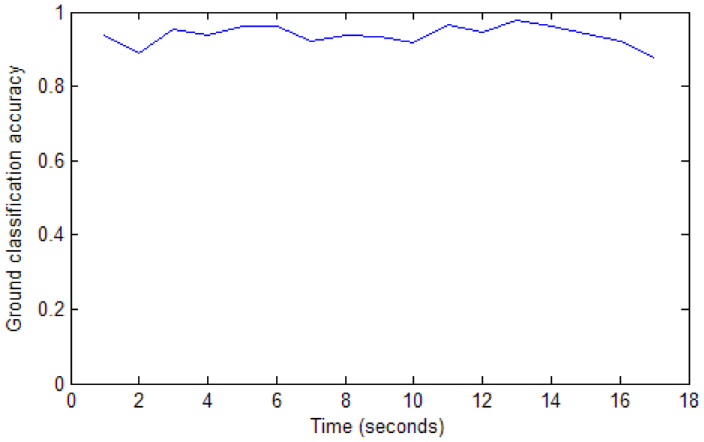
We implement the ground segmentation in 2D image every second. <xref ref-type="fig" rid="f12-sensors-12-11221">Figure 12</xref> shows the ground classification accuracy samples during the robot navigated in an unknown environment. The accuracy value is calculated as the ratio between the inferred ground pixels and the actual ground pixels.</p>
<p>
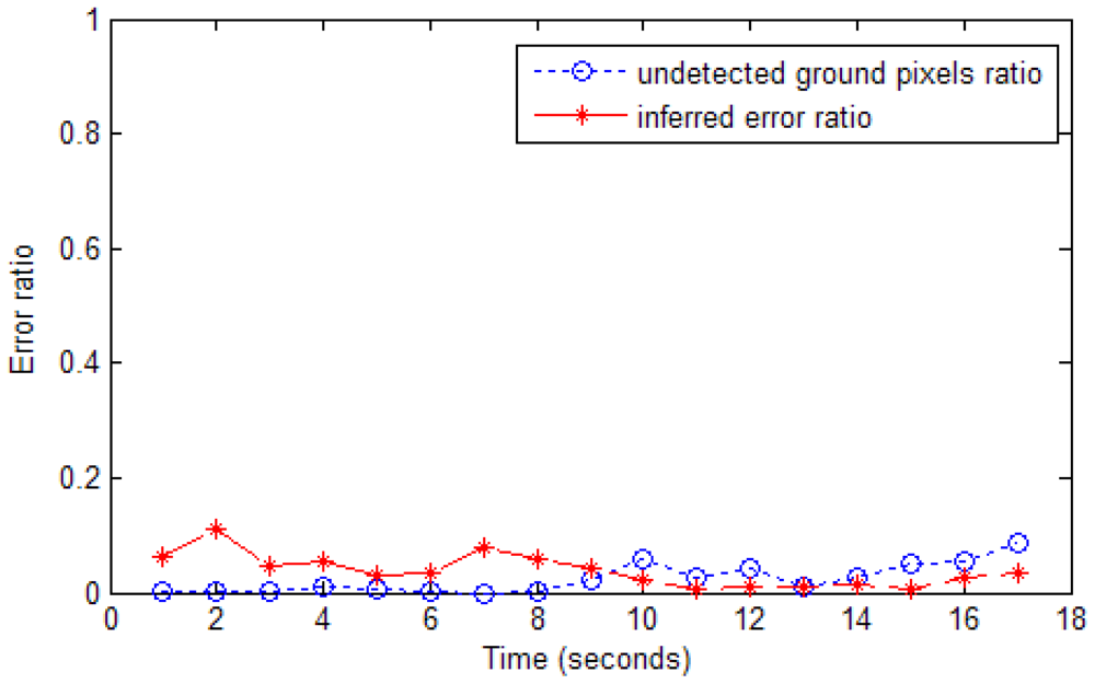
We define two types of classification errors in this project. One of them results from undetected ground pixels. If ground pixels are inferred as non-ground pixels, we define them as inferred errors. <xref ref-type="fig" rid="f13-sensors-12-11221">Figure 13</xref> shows samples of undetected ground pixel ratio and inferred error ratio.</p>
<p>
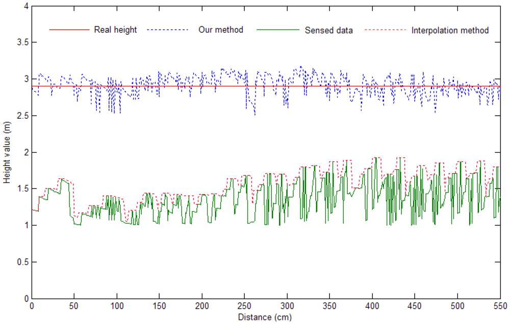
We then detect the edge of objects by using the non-ground classification result. We investigate the performance of the proposed height estimation method by comparing the obtained values with the actual heights (2.90 m on average). Since the range sensor scans objects only up to a height of 1.8 m, the upper parts of buildings cannot be sensed. However, as shown in <xref ref-type="fig" rid="f14-sensors-12-11221">Figure 14</xref>, we recover the missing parts from the incomplete terrain mesh, and the average estimated height value is 2.92 ± 0.11 m. In <xref ref-type="fig" rid="f14-sensors-12-11221">Figure 14</xref>, the <italic>x</italic>-axis represents the distance between the estimated vertices with the first estimated vertex.</p>
<p>The previously proposed interpolation algorithms average the empty region using the surrounding 3D points. These methods do not recover the actual shape of the unsensed region. However, using our proposed height estimation method, we successfully recover the actual shape of the missing parts.</p>
<p>
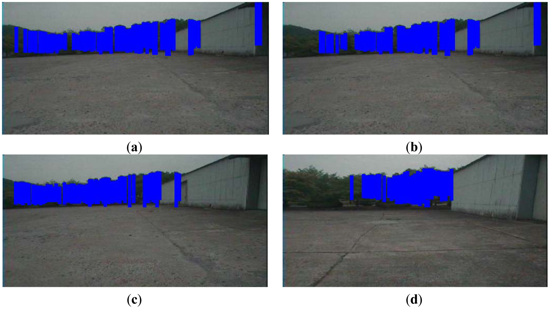
We render the textured terrain mesh and represent the texture of the ground, trees, and buildings at an average of 11.43 frames per second (FPS) using the Gibbs-MRF model along with the flood-fill algorithm. This is faster than the case where only the Gibbs-MRF model is used (8.37 FPS). After recovering complete scenes in the terrain mesh, we classify objects into tree and building classes. The tree classification results are indicated in blue color in the 2D images in <xref ref-type="fig" rid="f15-sensors-12-11221">Figure 15</xref>. In the 50th and 100th frames, the objects are located far from the robot, so that noise exists in the sensed objects, especially at the corners. When the robot moves closer to the building in the 200th frame, the corner shape is detected accurately. The corner pixels are grouped in the building class. When the robot is located near the trees in the 800th frame, the accuracy of the range sensor is higher than that when the robot is far from the trees. Finally, the noise in the spaces between the trees is removed in the reconstructed terrain mesh.</p>
<p>We use a manual supervised method to classify the pixels in the 2D images of <xref ref-type="fig" rid="f15-sensors-12-11221">Figure 15(a–d)</xref> into tree and building objects. By using the inferred results and through manual classification, the confusion matrices in <xref ref-type="table" rid="t2-sensors-12-11221">Tables 2</xref>–<xref ref-type="table" rid="t5-sensors-12-11221">5</xref> are obtained. When the robot moves closer to the objects, the spatial distribution of the objects is detected with low noise; in this case, object classification is performed correctly and the error ratio is low.</p></sec>
<sec sec-type="conclusions">
<label>5.</label>
<title>Conclusions</title>
<p>This paper described a method of effective segmentation of ground, buildings, and trees for automated surveying and mapping by mobile robots. The method was found effective in an outdoor environment for a mobile robot with a range sensor, video camera, GPS receiver, and a gyroscope.</p>
<p>The complete shape of objects that are partly outside sensors' range of measurement is accurately recovered. The accurate height estimation allowed successful classification of buildings and trees on the basis of their spatial distribution. However, the height estimation algorithm does not work well for recovering the buildings which are not uniform in color or have overhanging roofs. In future, we will improve the system to deal with these problems.</p></sec></body>
<back>
<ack>
<p>This work was supported by the Agency for Defense Development, South Korea.</p></ack>
<ref-list>
<title>References</title>
<ref id="b1-sensors-12-11221"><label>1.</label><citation citation-type="journal"><person-group person-group-type="author"><name><surname>Matsushita</surname><given-names>Y.</given-names></name><name><surname>Miura</surname><given-names>J.</given-names></name></person-group><article-title>On-line road boundary modeling with multiple sensory features, flexible road model, and particle filter</article-title><source>Robot. Auton. Syst.</source><year>2011</year><volume>59</volume><fpage>274</fpage><lpage>284</lpage><pub-id pub-id-type="doi">10.1016/j.robot.2011.02.009</pub-id></citation></ref>
<ref id="b2-sensors-12-11221"><label>2.</label><citation citation-type="confproc"><person-group person-group-type="author"><name><surname>SoundraPandian</surname><given-names>K.K.</given-names></name><name><surname>Mathur</surname><given-names>P.</given-names></name></person-group><article-title>Traversability Assessment of Terrain for Autonomous Robot Navigation</article-title><conf-name>Proceedings of the International MultiConference of Engineers and Computer Scientists</conf-name><conf-loc>Hong Kong, China</conf-loc><conf-date>17–19 March 2010</conf-date><comment>Volume 2</comment><fpage>17</fpage><lpage>20</lpage></citation></ref>
<ref id="b3-sensors-12-11221"><label>3.</label><citation citation-type="confproc"><person-group person-group-type="author"><name><surname>Sukumar</surname><given-names>S.R.</given-names></name><name><surname>Yu</surname><given-names>S.J.</given-names></name><name><surname>Page</surname><given-names>D.L.</given-names></name><name><surname>Koschan</surname><given-names>A.F.</given-names></name><name><surname>Abidi</surname><given-names>M.A.</given-names></name></person-group><article-title>Multi-Sensor Integration for Unmanned Terrain Modeling</article-title><conf-name>Proceedings of the SPIE Unmanned Systems Technology VIII</conf-name><conf-loc>Orlando, FL, USA</conf-loc><conf-date>17– 20 April 2006</conf-date><comment>Volume 6230</comment><fpage>65</fpage><lpage>74</lpage></citation></ref>
<ref id="b4-sensors-12-11221"><label>4.</label><citation citation-type="confproc"><person-group person-group-type="author"><name><surname>Huber</surname><given-names>D.</given-names></name><name><surname>Herman</surname><given-names>H.</given-names></name><name><surname>Kelly</surname><given-names>A.</given-names></name><name><surname>Rander</surname><given-names>P.</given-names></name><name><surname>Ziglar</surname><given-names>J.</given-names></name></person-group><article-title>Real-Time Photo-realistic Visualization of 3D Environments for Enhanced Tele-operation of Vehicles</article-title><conf-name>Proceedings of the International Conference on 3D Digital Imaging and Modeling (3DIM)</conf-name><conf-loc>Kyoto, Japan</conf-loc><conf-date>3–4 October 2009</conf-date><fpage>1518</fpage><lpage>1525</lpage></citation></ref>
<ref id="b5-sensors-12-11221"><label>5.</label><citation citation-type="journal"><person-group person-group-type="author"><name><surname>Saxena</surname><given-names>A.</given-names></name><name><surname>Chung</surname><given-names>S.H.</given-names></name><name><surname>Ng</surname><given-names>A.Y.</given-names></name></person-group><article-title>3-D depth reconstruction from a single still image</article-title><source>Int. J. Comput. Vis.</source><year>2008</year><volume>76</volume><fpage>53</fpage><lpage>69</lpage></citation></ref>
<ref id="b6-sensors-12-11221"><label>6.</label><citation citation-type="confproc"><person-group person-group-type="author"><name><surname>Kim</surname><given-names>G.H.</given-names></name><name><surname>Huber</surname><given-names>D.</given-names></name><name><surname>Hebert</surname><given-names>M.</given-names></name></person-group><article-title>Segmentation of Salient Regions in Outdoor Scenes Using Imagery and 3D Data</article-title><conf-name>Proceedings of the IEEE Workshop on Applications of Computer Vision (WACV08)</conf-name><conf-loc>Copper Mountain Resort, CO, USA</conf-loc><conf-date>7– 9 January 2008</conf-date><fpage>1</fpage><lpage>8</lpage></citation></ref>
<ref id="b7-sensors-12-11221"><label>7.</label><citation citation-type="journal"><person-group person-group-type="author"><name><surname>Früh</surname><given-names>C.</given-names></name><name><surname>Zakhor</surname><given-names>A.</given-names></name></person-group><article-title>Data processing algorithms for generating textured 3D building facade meshes from laser scans and camera images</article-title><source>Int. J. Comput. Vis.</source><year>2005</year><volume>61</volume><fpage>159</fpage><lpage>184</lpage><pub-id pub-id-type="doi">10.1023/B:VISI.0000043756.03810.dd</pub-id></citation></ref>
<ref id="b8-sensors-12-11221"><label>8.</label><citation citation-type="journal"><person-group person-group-type="author"><name><surname>Nüchter</surname><given-names>A.</given-names></name><name><surname>Hertzberg</surname><given-names>J.</given-names></name></person-group><article-title>Towards semantic maps for mobile robots</article-title><source>Robot. Auton. Syst.</source><year>2008</year><volume>56</volume><fpage>915</fpage><lpage>926</lpage><pub-id pub-id-type="doi">10.1016/j.robot.2008.08.001</pub-id></citation></ref>
<ref id="b9-sensors-12-11221"><label>9.</label><citation citation-type="journal"><person-group person-group-type="author"><name><surname>Kelly</surname><given-names>A.</given-names></name><name><surname>Chan</surname><given-names>N.</given-names></name><name><surname>Herman</surname><given-names>H.</given-names></name><name><surname>Huber</surname><given-names>D.</given-names></name><name><surname>Meyers</surname><given-names>R.</given-names></name><name><surname>Rander</surname><given-names>P.</given-names></name><name><surname>Warner</surname><given-names>R.</given-names></name><name><surname>Ziglar</surname><given-names>J.</given-names></name><name><surname>Capstick</surname><given-names>E.</given-names></name></person-group><article-title>Real-time photorealistic virtualized reality interface for remote mobile robot control</article-title><source>Int. J. Robot. Res.</source><year>2011</year><volume>30</volume><fpage>384</fpage><lpage>404</lpage><pub-id pub-id-type="doi">10.1177/0278364910383724</pub-id></citation></ref>
<ref id="b10-sensors-12-11221"><label>10.</label><citation citation-type="journal"><person-group person-group-type="author"><name><surname>Yu</surname><given-names>S.J.</given-names></name><name><surname>Sukumar</surname><given-names>S.R.</given-names></name><name><surname>Koschan</surname><given-names>A.F.</given-names></name><name><surname>Page</surname><given-names>D.L.</given-names></name><name><surname>Abidi</surname><given-names>M.A.</given-names></name></person-group><article-title>3D reconstruction of road surfaces using an integrated multi-sensory approach</article-title><source>Opt. Lasers Eng.</source><year>2007</year><volume>45</volume><fpage>808</fpage><lpage>818</lpage><pub-id pub-id-type="doi">10.1016/j.optlaseng.2006.12.007</pub-id></citation></ref>
<ref id="b11-sensors-12-11221"><label>11.</label><citation citation-type="journal"><person-group person-group-type="author"><name><surname>Schiewe</surname><given-names>J.</given-names></name></person-group><article-title>Integration of multi-sensor data for landscape modeling using a region-based approach</article-title><source>ISPRS J. Photogram. Remote Sens.</source><year>2003</year><volume>57</volume><fpage>371</fpage><lpage>379</lpage><pub-id pub-id-type="doi">10.1016/S0924-2716(02)00165-X</pub-id></citation></ref>
<ref id="b12-sensors-12-11221"><label>12.</label><citation citation-type="journal"><person-group person-group-type="author"><name><surname>Sequeira</surname><given-names>V.</given-names></name><name><surname>Ng</surname><given-names>K.</given-names></name><name><surname>Wolfart</surname><given-names>E.</given-names></name><name><surname>Gonçalves</surname><given-names>J.G.M.</given-names></name><name><surname>Hogg</surname><given-names>D.</given-names></name></person-group><article-title>Automated reconstruction of 3D models from real environments</article-title><source>J. Photogramm. Remote Sens.</source><year>1999</year><volume>54</volume><fpage>1</fpage><lpage>22</lpage><pub-id pub-id-type="doi">10.1016/S0924-2716(98)00026-4</pub-id></citation></ref>
<ref id="b13-sensors-12-11221"><label>13.</label><citation citation-type="journal"><person-group person-group-type="author"><name><surname>Rovira-Más</surname><given-names>F.</given-names></name><name><surname>Zhang</surname><given-names>Q.</given-names></name><name><surname>Reid</surname><given-names>J.F.</given-names></name></person-group><article-title>Stereo vision three-dimensional terrain maps for precision agriculture</article-title><source>Comput. Electron. Agric.</source><year>2008</year><volume>60</volume><fpage>133</fpage><lpage>143</lpage><pub-id pub-id-type="doi">10.1016/j.compag.2007.07.007</pub-id></citation></ref>
<ref id="b14-sensors-12-11221"><label>14.</label><citation citation-type="journal"><person-group person-group-type="author"><name><surname>Kraus</surname><given-names>K.</given-names></name><name><surname>Pfeifer</surname><given-names>N.</given-names></name></person-group><article-title>Determination of terrain models in wooded areas with airborne laser scanner data</article-title><source>J. Photogramm. Remote Sens.</source><year>1998</year><volume>53</volume><fpage>193</fpage><lpage>203</lpage><pub-id pub-id-type="doi">10.1016/S0924-2716(98)00009-4</pub-id></citation></ref>
<ref id="b15-sensors-12-11221"><label>15.</label><citation citation-type="journal"><person-group person-group-type="author"><name><surname>Huang</surname><given-names>Y.M.</given-names></name><name><surname>Chen</surname><given-names>C.J.</given-names></name></person-group><article-title>3D fractal reconstruction of terrain profile data based on digital elevation model</article-title><source>Chaos Soliton. Fractal.</source><year>2009</year><volume>40</volume><fpage>1741</fpage><lpage>1749</lpage><pub-id pub-id-type="doi">10.1016/j.chaos.2007.09.091</pub-id></citation></ref>
<ref id="b16-sensors-12-11221"><label>16.</label><citation citation-type="journal"><person-group person-group-type="author"><name><surname>Kobler</surname><given-names>A.</given-names></name><name><surname>Pfeifer</surname><given-names>N.</given-names></name><name><surname>Ogrinc</surname><given-names>P.</given-names></name><name><surname>Todorovski</surname><given-names>L.</given-names></name><name><surname>Oštir</surname><given-names>K.</given-names></name><name><surname>D(x0017E)eroski</surname><given-names>S.</given-names></name></person-group><article-title>Repetitive interpolation: A robust algorithm for DTM generation from aerial laser scanner data in forested terrain</article-title><source>Remote Sens. Environ.</source><year>2007</year><volume>108</volume><fpage>9</fpage><lpage>23</lpage><pub-id pub-id-type="doi">10.1016/j.rse.2006.10.013</pub-id></citation></ref>
<ref id="b17-sensors-12-11221"><label>17.</label><citation citation-type="journal"><person-group person-group-type="author"><name><surname>Hugentobler</surname><given-names>M.</given-names></name><name><surname>Schneider</surname><given-names>B.</given-names></name></person-group><article-title>Breaklines in Coons surfaces over triangles for the use in terrain modeling</article-title><source>Comput. Geosci.</source><year>2005</year><volume>31</volume><fpage>45</fpage><lpage>54</lpage><pub-id pub-id-type="doi">10.1016/j.cageo.2004.09.006</pub-id></citation></ref>
<ref id="b18-sensors-12-11221"><label>18.</label><citation citation-type="confproc"><person-group person-group-type="author"><name><surname>Douillard</surname><given-names>B.</given-names></name><name><surname>Brooks</surname><given-names>A.</given-names></name><name><surname>Ramos</surname><given-names>F.</given-names></name></person-group><article-title>A 3D Laser and Vision Based Classifier</article-title><conf-name>Proceedings of the Fifth International Conference on Intelligent Sensors, Sensor Networks and Information Processing</conf-name><conf-loc>Melbourne, Australia</conf-loc><conf-date>7–10 December 2009</conf-date><fpage>295</fpage><lpage>300</lpage></citation></ref>
<ref id="b19-sensors-12-11221"><label>19.</label><citation citation-type="journal"><person-group person-group-type="author"><name><surname>Wellington</surname><given-names>C.</given-names></name><name><surname>Courville</surname><given-names>A.</given-names></name><name><surname>Stentz</surname><given-names>A.</given-names></name></person-group><article-title>A generative model of terrain for autonomous navigation in vegetation</article-title><source>Int. J. Robot. Res.</source><year>2006</year><volume>25</volume><fpage>1287</fpage><lpage>1304</lpage><pub-id pub-id-type="doi">10.1177/0278364906072769</pub-id></citation></ref>
<ref id="b20-sensors-12-11221"><label>20.</label><citation citation-type="book"><person-group person-group-type="author"><name><surname>Kindermann</surname><given-names>R.</given-names></name><name><surname>Snell</surname><given-names>J.L.</given-names></name></person-group><source>Markov Random Fields and Their Applications</source><publisher-name>American Mathematical Society (AMS)</publisher-name><publisher-loc>Providence, RI, USA</publisher-loc><year>1980</year></citation></ref>
<ref id="b21-sensors-12-11221"><label>21.</label><citation citation-type="journal"><person-group person-group-type="author"><name><surname>Besag</surname><given-names>J.</given-names></name></person-group><article-title>Spatial interaction and the statistical analysis of lattice systems</article-title><source>J. R. Statist. Soc.</source><year>1974</year><volume>36</volume><fpage>192</fpage><lpage>236</lpage></citation></ref>
<ref id="b22-sensors-12-11221"><label>22.</label><citation citation-type="journal"><person-group person-group-type="author"><name><surname>Geman</surname><given-names>S.</given-names></name><name><surname>Geman</surname><given-names>D.</given-names></name></person-group><article-title>Stochastic relaxation, Gibbs distribution, and the Bayesian restoration of images</article-title><source>J. Appl. Statist.</source><year>1984</year><volume>6</volume><fpage>721</fpage><lpage>741</lpage></citation></ref>
<ref id="b23-sensors-12-11221"><label>23.</label><citation citation-type="confproc"><person-group person-group-type="author"><name><surname>Zeng</surname><given-names>W.</given-names></name><name><surname>Gao</surname><given-names>W.</given-names></name></person-group><article-title>Semantic Object Segmentation by a Spatio-Temporal MRF Model</article-title><conf-name>Proceedings of the International Conference on Pattern Recognition</conf-name><conf-loc>Cambridge, UK</conf-loc><conf-date>23–26 August 2004</conf-date><fpage>775</fpage><lpage>778</lpage></citation></ref>
<ref id="b24-sensors-12-11221"><label>24.</label><citation citation-type="journal"><person-group person-group-type="author"><name><surname>Perez</surname><given-names>P.</given-names></name></person-group><article-title>Markov random fields and images</article-title><source>CWI Q.</source><year>1998</year><volume>11</volume><fpage>413</fpage><lpage>437</lpage></citation></ref>
<ref id="b25-sensors-12-11221"><label>25.</label><citation citation-type="journal"><person-group person-group-type="author"><name><surname>Szirányi</surname><given-names>T.</given-names></name><name><surname>Zerubia</surname><given-names>J.</given-names></name><name><surname>Czúni</surname><given-names>L.</given-names></name><name><surname>Geldreich</surname><given-names>D.</given-names></name><name><surname>Kato</surname><given-names>Z.</given-names></name></person-group><article-title>Image segmentation using Markov random field model in fully parallel cellular network architectures</article-title><source>Real Time Imaging</source><year>2000</year><volume>6</volume><fpage>195</fpage><lpage>211</lpage><pub-id pub-id-type="doi">10.1006/rtim.1998.0159</pub-id></citation></ref>
<ref id="b26-sensors-12-11221"><label>26.</label><citation citation-type="confproc"><person-group person-group-type="author"><name><surname>Anguelov</surname><given-names>D.</given-names></name><name><surname>Taskarf</surname><given-names>B.</given-names></name><name><surname>Chatalbashev</surname><given-names>V.</given-names></name><name><surname>Koller</surname><given-names>D.</given-names></name><name><surname>Gupta</surname><given-names>D.</given-names></name><name><surname>Heitz</surname><given-names>G.</given-names></name><name><surname>Ng</surname><given-names>A.</given-names></name></person-group><article-title>Discriminative Learning of Markov Random Fields for Segmentation of 3D Scan Data</article-title><conf-name>Proceedings of the IEEE Computer Society Conference on Computer Vision and Pattern Recognition</conf-name><conf-loc>San Diego, CA, USA</conf-loc><conf-date>20– 25 June 2005</conf-date><fpage>169</fpage><lpage>176</lpage></citation></ref>
<ref id="b27-sensors-12-11221"><label>27.</label><citation citation-type="journal"><person-group person-group-type="author"><name><surname>Weiss</surname><given-names>U.</given-names></name><name><surname>Biber</surname><given-names>P.</given-names></name></person-group><article-title>Plant detection and mapping for agricultural robots using a 3D LIDAR sensor</article-title><source>Robot. Auton. Syst.</source><year>2011</year><volume>59</volume><fpage>265</fpage><lpage>273</lpage><pub-id pub-id-type="doi">10.1016/j.robot.2011.02.011</pub-id></citation></ref>
<ref id="b28-sensors-12-11221"><label>28.</label><citation citation-type="confproc"><person-group person-group-type="author"><name><surname>Golovinskiy</surname><given-names>A.</given-names></name><name><surname>Funkhouser</surname><given-names>T.</given-names></name></person-group><article-title>Min-Cut Based Segmentation of Point Clouds</article-title><conf-name>Proceedings of the IEEE 12th International Conference on Computer Vision Workshops (ICCV Workshops)</conf-name><conf-loc>Kyoto, Japan</conf-loc><conf-date>27 September– 4 October 2009</conf-date><fpage>39</fpage><lpage>46</lpage></citation></ref>
<ref id="b29-sensors-12-11221"><label>29.</label><citation citation-type="journal"><person-group person-group-type="author"><name><surname>Lalonde</surname><given-names>J.-F.</given-names></name><name><surname>Vandapel</surname><given-names>N.</given-names></name><name><surname>Hebert</surname><given-names>M.</given-names></name></person-group><article-title>Natural terrain classification using three-dimensional ladar data for ground robot mobility</article-title><source>J. Field Robot.</source><year>2006</year><volume>3</volume><fpage>839</fpage><lpage>861</lpage></citation></ref>
<ref id="b30-sensors-12-11221"><label>30.</label><citation citation-type="confproc"><person-group person-group-type="author"><name><surname>Huber</surname><given-names>D.</given-names></name><name><surname>Akinci</surname><given-names>B.</given-names></name><name><surname>Oliver</surname><given-names>A.A.</given-names></name><name><surname>Anil</surname><given-names>E.</given-names></name><name><surname>Okorn</surname><given-names>B.E.</given-names></name><name><surname>Xiong</surname><given-names>X.H.</given-names></name></person-group><article-title>Methods for Automatically Modeling and Representing As-Built Building Information Models</article-title><conf-name>Proceedings of the NSF CMMI Research Innovation Conference</conf-name><conf-loc>Atlanta, GA, USA</conf-loc><conf-date>4–7 January 2011</conf-date></citation></ref></ref-list>
<sec sec-type="display-objects">
<title>Figures and Tables</title>
<fig id="f1-sensors-12-11221" position="float">
<label>Figure 1.</label>
<caption>
<p>Framework for outdoor terrain reconstruction and object classification.</p></caption>
<graphic xlink:href="sensors-12-11221f1.gif"/></fig>
<fig id="f2-sensors-12-11221" position="float">
<label>Figure 2.</label>
<caption>
<p>Grid-based ground modeling.</p></caption>
<graphic xlink:href="sensors-12-11221f2.gif"/></fig>
<fig id="f3-sensors-12-11221" position="float">
<label>Figure 3.</label>
<caption>
<p>Rough segmentation of 3D ground data.</p></caption>
<graphic xlink:href="sensors-12-11221f3.gif"/></fig>
<fig id="f4-sensors-12-11221" position="float">
<label>Figure 4.</label>
<caption>
<p>Projection results as green pixels in an image.</p></caption>
<graphic xlink:href="sensors-12-11221f4.gif"/></fig>
<fig id="f5-sensors-12-11221" position="float">
<label>Figure 5.</label>
<caption>
<p>Terrain reconstruction results.</p></caption>
<graphic xlink:href="sensors-12-11221f5.gif"/></fig>
<fig id="f6-sensors-12-11221" position="float">
<label>Figure 6.</label>
<caption>
<p>Boundary searching in 2D image.</p></caption>
<graphic xlink:href="sensors-12-11221f6.gif"/></fig>
<fig id="f7-sensors-12-11221" position="float">
<label>Figure 7.</label>
<caption>
<p>Height estimation process.</p></caption>
<graphic xlink:href="sensors-12-11221f7.gif"/></fig>
<fig id="f8-sensors-12-11221" position="float">
<label>Figure 8.</label>
<caption>
<p>Reconstruction result after complete scene recovery. The recovered parts are indicated by the red rectangle.</p></caption>
<graphic xlink:href="sensors-12-11221f8.gif"/></fig>
<fig id="f9-sensors-12-11221" position="float">
<label>Figure 9.</label>
<caption>
<p>Spatial distributions of buildings and trees.</p></caption>
<graphic xlink:href="sensors-12-11221f9.gif"/></fig>
<fig id="f10-sensors-12-11221" position="float">
<label>Figure 10.</label>
<caption>
<p>Line detector masks.</p></caption>
<graphic xlink:href="sensors-12-11221f10.gif"/></fig>
<fig id="f11-sensors-12-11221" position="float">
<label>Figure 11.</label>
<caption>
<p>Segmentation and classification results. (<bold>a</bold>) Complete scene recovery. (<bold>b</bold>) Ground segmentation in the terrain mesh. (<bold>c</bold>) Tree classification in the terrain mesh. (<bold>d</bold>) Building classification in the terrain mesh.</p></caption>
<graphic xlink:href="sensors-12-11221f11.gif"/></fig>
<fig id="f12-sensors-12-11221" position="float">
<label>Figure 12.</label>
<caption>
<p>Ground classification accuracy.</p></caption>
<graphic xlink:href="sensors-12-11221f12.gif"/></fig>
<fig id="f13-sensors-12-11221" position="float">
<label>Figure 13.</label>
<caption>
<p>Errors in ground classification.</p></caption>
<graphic xlink:href="sensors-12-11221f13.gif"/></fig>
<fig id="f14-sensors-12-11221" position="float">
<label>Figure 14.</label>
<caption>
<p>Height estimation result.</p></caption>
<graphic xlink:href="sensors-12-11221f14.gif"/></fig>
<fig id="f15-sensors-12-11221" position="float">
<label>Figure 15.</label>
<caption>
<p>Tree classification results: (<bold>a</bold>) frame 50; (<bold>b</bold>) frame 100; (<bold>c</bold>) frame 200; and (<bold>d</bold>) frame 800.</p></caption>
<graphic xlink:href="sensors-12-11221f15.gif"/></fig>
<table-wrap id="t1-sensors-12-11221" position="float">
<label>Table 1.</label>
<caption>
<p>Ground segmentation performance.</p></caption>
<table frame="hsides" rules="groups">
<thead>
<tr>
<th align="center" valign="top"><bold>Truth/Inferred</bold></th>
<th align="center" valign="top">
<mml:math id="mm25" display="inline">
<mml:semantics id="sm25">
<mml:mrow>
<mml:mover accent="true">
<mml:mrow>
<mml:mtext mathvariant="italic">ground</mml:mtext></mml:mrow>
<mml:mo>¯</mml:mo></mml:mover></mml:mrow></mml:semantics></mml:math></th>
<th align="center" valign="top">
<mml:math id="mm26" display="inline">
<mml:semantics id="sm26">
<mml:mrow>
<mml:mover accent="true">
<mml:mrow>
<mml:mtext mathvariant="italic">non</mml:mtext>
<mml:mo>−</mml:mo>
<mml:mtext mathvariant="italic">ground</mml:mtext></mml:mrow>
<mml:mo>¯</mml:mo></mml:mover></mml:mrow></mml:semantics></mml:math></th></tr></thead>
<tbody>
<tr>
<td align="center" valign="top"><italic>ground</italic></td>
<td align="center" valign="top">67977</td>
<td align="center" valign="top">1611</td></tr>
<tr>
<td align="center" valign="top"><italic>non</italic> – <italic>ground</italic></td>
<td align="center" valign="top">2580</td>
<td align="center" valign="top">58904</td></tr></tbody></table></table-wrap>
<table-wrap id="t2-sensors-12-11221" position="float">
<label>Table 2.</label>
<caption>
<p>Tree classification result for <xref ref-type="fig" rid="f15-sensors-12-11221">Figure 15(a)</xref>.</p></caption>
<table frame="hsides" rules="groups">
<thead>
<tr>
<th align="center" valign="top"><bold>Truth/Inferred</bold></th>
<th align="center" valign="top">
<mml:math id="mm27" display="inline">
<mml:semantics id="sm27">
<mml:mrow>
<mml:mover accent="true">
<mml:mrow>
<mml:mtext mathvariant="italic">tree</mml:mtext></mml:mrow>
<mml:mo>¯</mml:mo></mml:mover></mml:mrow></mml:semantics></mml:math></th>
<th align="center" valign="top">
<mml:math id="mm28" display="inline">
<mml:semantics id="sm28">
<mml:mrow>
<mml:mover accent="true">
<mml:mrow>
<mml:mtext mathvariant="italic">building</mml:mtext></mml:mrow>
<mml:mo>¯</mml:mo></mml:mover></mml:mrow></mml:semantics></mml:math></th></tr></thead>
<tbody>
<tr>
<td align="center" valign="top"><italic>tree</italic></td>
<td align="center" valign="top">9918</td>
<td align="center" valign="top">3026</td></tr>
<tr>
<td align="center" valign="top"><italic>building</italic></td>
<td align="center" valign="top">2828</td>
<td align="center" valign="top">10235</td></tr></tbody></table></table-wrap>
<table-wrap id="t3-sensors-12-11221" position="float">
<label>Table 3.</label>
<caption>
<p>Tree classification result for <xref ref-type="fig" rid="f15-sensors-12-11221">Figure 15(b)</xref>.</p></caption>
<table frame="hsides" rules="groups">
<thead>
<tr>
<th align="center" valign="top"><bold>Truth/Inferred</bold></th>
<th align="center" valign="top">
<mml:math id="mm29" display="inline">
<mml:semantics id="sm29">
<mml:mrow>
<mml:mover accent="true">
<mml:mrow>
<mml:mtext mathvariant="italic">tree</mml:mtext></mml:mrow>
<mml:mo>¯</mml:mo></mml:mover></mml:mrow></mml:semantics></mml:math></th>
<th align="center" valign="top">
<mml:math id="mm30" display="inline">
<mml:semantics id="sm30">
<mml:mrow>
<mml:mover accent="true">
<mml:mrow>
<mml:mtext mathvariant="italic">building</mml:mtext></mml:mrow>
<mml:mo>¯</mml:mo></mml:mover></mml:mrow></mml:semantics></mml:math></th></tr></thead>
<tbody>
<tr>
<td align="center" valign="top"><italic>tree</italic></td>
<td align="center" valign="top">11983</td>
<td align="center" valign="top">3106</td></tr>
<tr>
<td align="center" valign="top"><italic>building</italic></td>
<td align="center" valign="top">1749</td>
<td align="center" valign="top">9847</td></tr></tbody></table></table-wrap>
<table-wrap id="t4-sensors-12-11221" position="float">
<label>Table 4.</label>
<caption>
<p>Tree classification result for <xref ref-type="fig" rid="f15-sensors-12-11221">Figure 15(c)</xref>.</p></caption>
<table frame="hsides" rules="groups">
<thead>
<tr>
<th align="center" valign="top"><bold>Truth/Inferred</bold></th>
<th align="center" valign="top">
<mml:math id="mm31" display="inline">
<mml:semantics id="sm31">
<mml:mrow>
<mml:mover accent="true">
<mml:mrow>
<mml:mtext mathvariant="italic">tree</mml:mtext></mml:mrow>
<mml:mo>¯</mml:mo></mml:mover></mml:mrow></mml:semantics></mml:math></th>
<th align="center" valign="top">
<mml:math id="mm32" display="inline">
<mml:semantics id="sm32">
<mml:mrow>
<mml:mover accent="true">
<mml:mrow>
<mml:mtext mathvariant="italic">building</mml:mtext></mml:mrow>
<mml:mo>¯</mml:mo></mml:mover></mml:mrow></mml:semantics></mml:math></th></tr></thead>
<tbody>
<tr>
<td align="center" valign="top"><italic>tree</italic></td>
<td align="center" valign="top">11536</td>
<td align="center" valign="top">905</td></tr>
<tr>
<td align="center" valign="top"><italic>building</italic></td>
<td align="center" valign="top">1238</td>
<td align="center" valign="top">14652</td></tr></tbody></table></table-wrap>
<table-wrap id="t5-sensors-12-11221" position="float">
<label>Table 5.</label>
<caption>
<p>Tree classification result for <xref ref-type="fig" rid="f15-sensors-12-11221">Figure 15(d)</xref>.</p></caption>
<table frame="hsides" rules="groups">
<thead>
<tr>
<th align="center" valign="top"><bold>Truth/Inferred</bold></th>
<th align="center" valign="top">
<mml:math id="mm33" display="inline">
<mml:semantics id="sm33">
<mml:mrow>
<mml:mover accent="true">
<mml:mrow>
<mml:mtext mathvariant="italic">tree</mml:mtext></mml:mrow>
<mml:mo>¯</mml:mo></mml:mover></mml:mrow></mml:semantics></mml:math></th>
<th align="center" valign="top">
<mml:math id="mm34" display="inline">
<mml:semantics id="sm34">
<mml:mrow>
<mml:mover accent="true">
<mml:mrow>
<mml:mtext mathvariant="italic">building</mml:mtext></mml:mrow>
<mml:mo>¯</mml:mo></mml:mover></mml:mrow></mml:semantics></mml:math></th></tr></thead>
<tbody>
<tr>
<td align="center" valign="top"><italic>tree</italic></td>
<td align="center" valign="top">17196</td>
<td align="center" valign="top">33</td></tr>
<tr>
<td align="center" valign="top"><italic>building</italic></td>
<td align="center" valign="top">340</td>
<td align="center" valign="top">17771</td></tr></tbody></table></table-wrap></sec></back></article>
