The probability of a successful reception of a packet is the probability of successfully receiving all its bits, assuming that there is no error correction. It is well known that the probability of bit error depends on the encoding and modulation of the radio signal, thus, the packet reception probability will also depend on them. For example, for QPSK and BPSK modulation schemes, the packet reception probability in presence of additive white Gaussian noise and in absence of interferers is given by [24]: (1) PRP = ( 1 − BER ) 8 l = ( 1 − Q ( 2 E b N 0 ) ) 8 l = ( 1 − Q ( 2 snr ⋅ W v b ) ) 8 lwhere l is the length of the packet (in bytes), BER is the bit error rate, E_b/N₀ is the signal to noise ratio per bit, snr is the signal to noise ratio (in natural units), W is the channel bandwidth, v_b is the bit rate and the function Q(x) is the tail probability of the standard normal distribution.

More complete models have been proposed [25] to take into account complex phenomena such as asymmetry, interference, different quality of receivers and transmitters, correlations between reception rate of links, etc. However, this simpler model has been selected for this work because it enables a closed-form mathematical formulation and also fits quite well to experimental data (see Section 5.1).

On the other hand, a model of the channel that relates the transmission power to the received power is needed, as it will provide a relation between transmission power P_TX and SNR at the receiver for a certain distance between them. Many channel models have been proposed for outdoor and indoor environments [26] (e.g., Nakagami fading model, Rayleigh fading, Ricean fading, etc.) but one of the most popular, due to its simplicity, is the log-normal shadowing path loss model [27], which establishes the following relation between the received power (P_RX) and the distance (d) between transmitter and receiver: (2) P RX ( dBm ) = p TX ( dBm ) + A − 10 η log d d 0 + 𝒱where P_TX is the transmission power, A is a constant term, η is the path loss exponent, and ∼ (0, σ²) is a zero-mean Gaussian random variable with standard deviation σ. The constant term A depends on the transmitter's and receiver's antenna gains and on the power loss for a reference distance d₀, and has to be experimentally determined. On the other hand, the path loss exponent η typically ranges between 2 and 4 depending on the environment, and it has to be experimentally determined too. The random variable models the effects of shadowing and considers the randomness across an ensemble of many deployment environments. As the experiments in [28] indicate, if the environment is static and the transmitter and receiver stay at fixed positions, the standard deviation of the measured received power is lower than σ, whereas if a node moves or the environment changes (due to people movement or long lags of time) the standard deviation of the measured received power is σ. For this reason, if a channel model like Equation (2) is used to estimate distances, averaging a number of received signal strength measurements in a static situation does not significantly reduce the estimation errors, whereas averaging measurements taken at slightly different positions or in a changing environment is more effective to reduce estimation errors [29].

As previously said, this channel model provides a relation between the transmitted power (P_TX), the SNR at the receiver and the distance (d) between transmitter and receiver, i.e.,: (3) SNR ( d B ) = P TX ( dBm ) + A − 10 η log d d 0 − N RX ( dBm ) + 𝒱where SNR, which is a random variable, is the signal to noise ratio at the receiver expressed in decibels and N_RX is the noise level at the receiver.

Let us consider a certain link of a network like the one described in Section 3, consisting of a transmitter node, which will periodically send packets, and a receiver node, which will measure the RSS or the TOA of all received packets. The receiver will average all the measurements (n) obtained during the localization period T₀, so that the standard deviation of the measurements can be reduced by a factor of n. Therefore, a desired accuracy in the measurement of the RSS or the TOA imposes a minimum number of received packets n_obj.

On the other hand, when k packets are transmitted, the average number of packets that are finally received is: (4) n = k ⋅ PRP = T 0 T ⋅ PRPwhere T is the time interval between consecutive transmitted packets. Consequently, a desired accuracy in the RSS or the TOA imposes a relationship between T and PRP, given T₀. As shown in Section 3.1, the PRP depends on the snr at the receiver. As a result, a desired accuracy imposes a relationship between snr and T. Among all snr-T pairs that ensure the required number of received packets, we want to find the one with the lowest energy consumption.

The consumed energy at transmission during T₀ is given by: (5) E TX = k ⋅ E p = k ⋅ p tx ⋅ T p = n ⋅ p tx ⋅ T p PRPwhere k is the number of transmitted packets during the period T₀, E_p is the consumed energy when transmitting a single packet, p_tx is the transmission power (in natural units), T_p is the time it takes to send a packet and n is the average number of received packets. Since the localization procedure is periodic with period T₀, this consumed energy is an appropriate parameter to analyze the energy efficiency.

If we assume that the receiver is awake and listening to possible receptions only at given periods (previously negotiated with the transmitter), the consumed energy at reception during T₀ is given by: (6) E RX = C rx ⋅ T rwhere T_r is the reception period and C_rx is the consumption when the node is in receiving mode. E_RX is constant, as C_rx is a constant value that depends on the hardware characteristics. Therefore, in order to minimize the total energy consumption, we will only need to minimize the energy consumption during transmission.

Using Equations (1) and (3), E_TX can be expressed as a function of the signal to noise ratio at the receiver: (7) E TX = n T p v b d η n rx 2 W a ⋅ x 2 ( 1 − Q ( x ) ) 8 l ⋅ χwhere n_rx and a are N_RX and A expressed in natural units, χ is a log-normal random variable with parameters μ_χ = 0 and σ_χ = σ · ln 10/10, and x is given by: (8) x = 2 snr W v bwhere snr is the mean value of the SNR expressed in natural units.

It can be obviously noticed that, for a given distance, the greater the required accuracy (described by n), the more energy will be consumed. On the other hand, as the distance between transmitter and receiver increases, the consumed energy increases as well, for a given desired accuracy. Finally, note that E_TX is a random variable composed of a constant multiplied by a log-normal random variable, therefore, it is itself another log-normal random variable, with parameters μ E = ln ( n T p v b d η n rx 2 W a x 2 ( 1 − Q ( x ) ) 8 l ), σ_E = σ_χ and mean value given by: (9) E ¯ TX = n T p v b d η n rx 2 W a ⋅ x 2 ( 1 − Q ( x ) ) 8 l ⋅ e 1 2 ( σ ⋅ ln 10 10 ) 2

Deriving Equation (9) with respect to the snr at the receiver, it can be obtained that the value of x (or snr) for which the average energy consumption reaches a minimum (x*) satisfies the following expression: (10) x ∗ e − x ∗ 2 / 2 ( 1 − Q ( x ∗ ) ) = 2 π 4 l

In conclusion, if we manage to achieve the snr* corresponding to this x*, the energy consumption will be minimized.

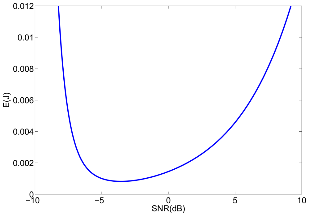
To provide some illustrative results, Figure 1 shows the energy consumption as a function of the SNR for the parameters of our sensor network, which performs a localization once a second, that is, T₀ = 1 s, and uses 8-bytes packets, with T_p = 256 μs. The estimated values of the channel parameters are η = 2.5 and A = −80 dBm and the noise level at the receiver is N_RX = −87 dBm. The energy consumption was calculated for n = 5 and d = 2 m. We can see in Figure 1 that if the optimum SNR value is not achievable, it would be better to use a higher transmission power, as the increase of power consumption with the SNR is slower for higher values of SNR.

On the other hand, note that the desired accuracy imposed a relationship between snr and T, thus, there is an optimum value of T corresponding to snr*, which can be calculated from Equations (1) and (4): (11) T ∗ = T 0 n ⋅ ( 1 − Q ( 2 snr ∗ ⋅ W v b ) ) 8 l

In conclusion, among the pairs snr-T that satisfy a desired accuracy, there is a pair snr*-T* for which the energy consumption is minimum. For that reason, in order to measure the RSS or the TOA with certain accuracy, the strategy that we propose consists in transmitting packets with a packet rate of 1/T* and such a transmission power P_TX that the snr at the receiver is equal to snr*. As the snr at the receiver is proportional to the transmission power for a given distance d between transmitter and receiver (see Section 3.2), in order to calculate the optimum value of P_TX, an estimate of the distance between transmitter and receiver is needed. In practice, this distance estimation can be obtained from the RSS or TOA measurements of the previous localization period.

Note (from Equation (10)) that the optimum value x* only depends on the packet length, therefore, the optimum value of snr at the receiver to achieve the lowest energy consumption does not depend on the accuracy we want to obtain or on the propagation characteristics, it only depends on the packet length and on the W/v_b ratio, i.e., its value is constant for a given network. This is an interesting result from a practical point of view, as it implies that the value of snr* does not need to be calculated in real time, which would be costly from a computational point of view, as it involves solving expression (10) iteratively. Therefore, the proposed strategy only involves very simple operations to calculate the optimum values of T* and P TX ∗ from the known value of snr* and, yet, guarantees the desired accuracy in the measurements while achieving the minimum energy consumption. This results in a very useful and attractive technique for battery-powered wireless devices that are deployed to perform the localization of people or objects. Although we have derived here the particular expressions for the specific case of our channel and receiver models, the strategy is directly extendable to other models.

Let us also remark that the value of the localization period T₀ does not have any influence on the applicability of our strategy as long as it is big enough to send the required number of packets, which is usually the case in practice. Furthermore, the value of T₀ does not need to be constant in time. In fact, it can be optimized to adapt to the mobility characteristics of the mobile node [15–18]. The combination of the proposed optimization with the optimization of the localization period may lead to further energy savings.

Note that as we have assumed that there is a synchronization schedule known by all the nodes, the localization messages should be sent within the assigned periods. In principle, this does not affect the localization accuracy or the proposed strategy, as long as the required number of packets can be transmitted.

Finally, we would like to point out that in practice, the synchronization of the network may not be perfect. In this case, the nodes should be listening to possible transmissions also during the idle periods in order not to lose packets, so the energy consumption in reception mode would increase. The proposed strategy is not directly affected, as it optimizes the energy consumption in transmission mode, but the energy savings, relative to the total energy consumption, would not be as high as in the ideal synchronization case. Another effect of an imperfect synchronization is that TOA measurements will not be so accurate, so its standard deviation will increase and the distance estimation errors will be higher. This does not affect the performance of the proposed strategy, as it was formulated in terms of the desired number of packets. But clearly, the desired number of packets to achieve a certain accuracy will increase with respect to the ideal case (see Equation (25) in Appendix A: if σ_t increases, n has to increase to achieve the same σ), and the energy consumption will increase accordingly.

In a real environment, the random nature of the propagation channel will have some effects on the proposed strategy that should be overcome. In particular, both the transmission power and the packet transmission rate need to be modified in order to maintain the desired accuracy when real propagation conditions are considered. In the rest of this section, we explain how and why these two parameters of the transmission strategy have to be corrected.

On one hand, the proposed strategy relies on the calculation of the transmission power that is necessary to reach the receiver with the optimum snr. As commented previously, an estimation of the distance between the nodes is necessary for this calculation. In real deployments, the distance estimations calculated from TOA or RSS measurements are affected by errors (see Appendix A and B), so the transmission power that is used to reach the receiver with the desired snr may be different from the optimum (see Section 4.3 for an analysis of how this fact affects the consumed energy). For example, in the case of RSS-based localization, in which distances are estimated from the received signal strength of the received packets, distances are usually underestimated. The reason is that the packets with low snr suffer from a higher loss probability and, thus, it is more probable to estimate the distance from higher-power packets, which will yield shorter distance estimations. If the transmission power corresponding to this underestimated distances is used, the packets will arrive at the receiver with a snr lower than snr*, and consequently, there will be more packet losses than desired. In order to avoid this effect, the transmission power has to be corrected.

According to Equation (3), the SNR (in decibels) of the packets that arrive at the receiver follows a normal distribution with mean SNR ¯ = P TX + A − 10 η log d / d 0 − N RX and standard deviation σ. Therefore, in natural units, the snr of these packets will be a log-normal random variable with parameters μ snr = SNR ¯ ⋅ ln 10 / 10 = ln 10 SNR ¯ / 10 and σ_snr = σ · ln 10/10. Among all the packets that reach the receiver, some are successfully received but some are not and the probability of a successful reception depends on the value of the snr, according to Equation (1). Thus, the probability density function of the snr given that the packet has been received can be expressed by: (12) f snr / rx ( snr ) = f snr ( snr ) ⋅ PRP ( snr ) ∫ − ∞ + ∞ f snr ( snr ) ⋅ PRP ( snr ) ⋅ d snr = 1 snr ⋅ σ snr 2 π ⋅ e − ( ln snr − μ snr ) 2 2 σ snr 2 ⋅ ( 1 − Q ( 2 snr ⋅ W v b ) ) 8 l ∫ − ∞ + ∞ 1 snr ⋅ σ snr 2 π ⋅ e − ( ln snr − μ snr ) 2 2 σ snr 2 ⋅ ( 1 − Q ( 2 snr ⋅ W v b ) ) 8 l d snr

If one of the received packets is used to estimate the distance, the difference between the transmission power necessary to reach the receiver with the desired snr* calculated from it (P̃_TX) and the optimum transmission power (given by the true distance) ( P TX ∗ ) can be expressed as: (13) P TX ∗ − P ∼ TX = SNR − SNR ∗where SNR refers here to the SNR of the successfully received packet, whose probability density function can be calculated from Equation (12), knowing that SNR = 10 · log snr: (14) f SNR / rx ( SNR ) = f SNR / rx ( SNR ) ∂ SNR ∂ snr = ln 10 10 ⋅ 10 SNR / 10 ⋅ f snr / rx ( SNR )

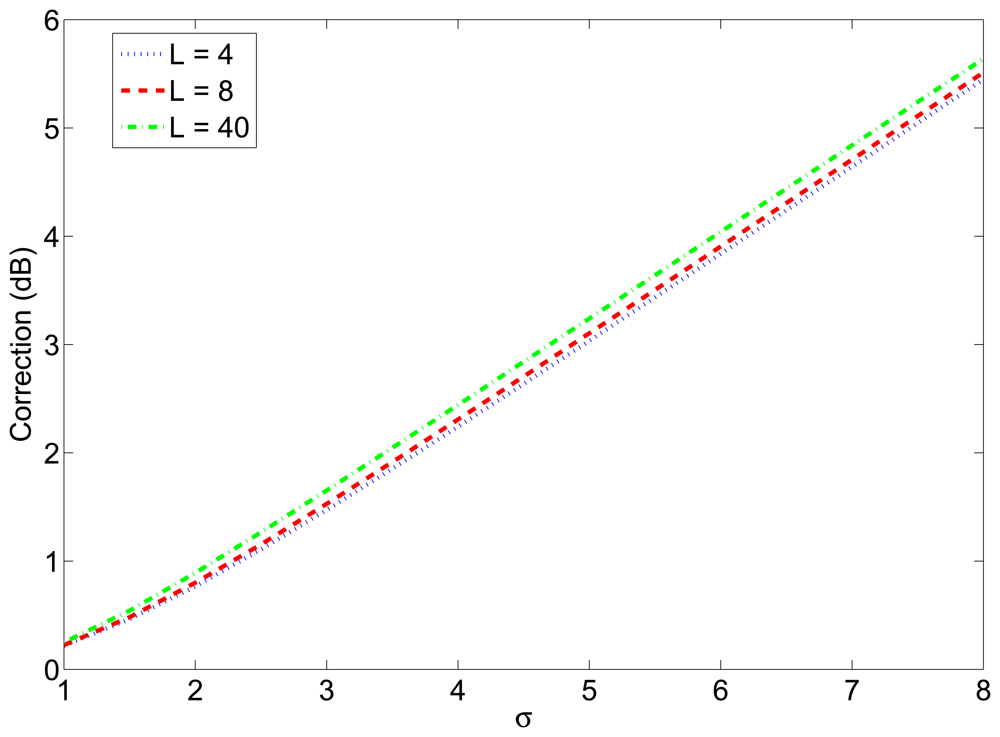
As a consequence, the estimated transmission power has to be corrected by adding a margin equal to the mean value of Equation (13). In other words, this margin must be calculated as the difference between the mean value of the SNR of the successfully received packets (which can be calculated numerically using Equation (14)) and SNR*. Figure 2 shows the value of this margin as a function of the standard deviation of the shadowing for different packet lengths. This margin was seen to be independent of the value of W/v_b, and nearly independent of the packet length, as it can be seen in the figure.

On the other hand, even when the optimum transmission power is used, the final snr at the receiver may not be the desired one, as the propagation is again affected by random shadowing. In fact, the snr at the receiver will be a log-normal random variable and, therefore, the PRP and n will also be random variables and their probability density functions can be calculated easily according to Equations (1) and (4). In particular, the probability density function of the PRP can be calculated as: (15) f PRP = f snr ∂ PRP ∂ snr = 2 π v b 8 l W ⋅ x ( 1 − Q ( x ) ) PRP ⋅ e x 2 / 2 ⋅ 1 snr ⋅ σ snr 2 π ⋅ e − ( ln snr − μ snr ) 2 2 σ snr 2where μ SNR = ln 10 SNR ¯ / 10 = ln snr ∗, σ_snr = σ · ln 10/10, x = 2 snr ⋅ W / v b and snr = v_b/2W · (Q⁻¹ (1 − PRP^1/8l)). Thus, knowing that n = k · PRP, the probability density function of n can be calculated as: (16) f n ( n ) = k ⋅ f PRP ( n ) = n obj PRP ∗ ⋅ f PRP ( n )where n_obj is the desired number of received packets and PRP* is the value of the packet reception probability corresponding to the optimum snr: PRP ∗ = ( 1 − Q ( 2 snr ∗ ⋅ W v b ) ) 8 l. The mean value of n can be then calculated numerically, resulting that this value is lower than the desired one n_obj. The difference between the two depends on l and W/v_b: the mean value of n is lower when the packet is longer or when W/v_b is higher. Figure 3 shows the relation between these two values for different values of l and W/vb for the case of RSS-based localization as a function of the standard deviation of the SNR distribution. This factor must be used to correct the number of transmitted packets, in order to counteract the effects of the propagation in real deployments. Thus, the estimated value of T* calculated from Equation (11) must be divided by this factor.

Although the energy consumption will increase when these two corrections are included in the transmission strategy, they are necessary to achieve the desired number of received packets in real environments and, therefore, to achieve the desired accuracy; otherwise, the accuracy would not be guaranteed. Nevertheless, the final energy consumption is very small and still entails significant savings with respect to other transmission strategies.

It is interesting to analyze how much energy will be consumed if the best transmission strategy is not perfectly achieved, due to an error in the estimated transmission power. As it has been mentioned above, the error in the estimated transmission power is due to an error in the distance estimation, which depends itself on the RSS or TOA measurement errors and on the number of packets that are averaged at the receiver. In this section, we first evaluate how the energy consumption is affected by the errors in the estimated transmission power and then we study how the distance estimation errors propagate to errors in the estimated transmission power, and therefore affect the energy consumption.

Let us suppose a transmitter node X that has to send packets to another node Y, so that Y receives in average n_obj packets during the period T₀. As the optimum snr at receiver node Y is known, node X can calculate the optimum value of T (T*) that satisfies the desired accuracy using Equation (11). On the other hand, the optimum transmission power P TX ∗ can be obtained from Equation (3), assuming that the distance between transmitter node X and receiver node Y is known. An error in the distance estimation will produce an error in the estimated optimum transmission power, which will lead to the use of a transmission power P TX ′ different from the optimum P TX ∗. If the estimated transmission power is greater than P TX ∗, the energy consumption will increase with respect to the minimum E_min and the number of received packets will increase as well with respect to n_obj, although it is not necessary. If the estimated transmission power is lower than P TX ∗, the energy consumption will diminish, but the number of received packets will not be sufficient.

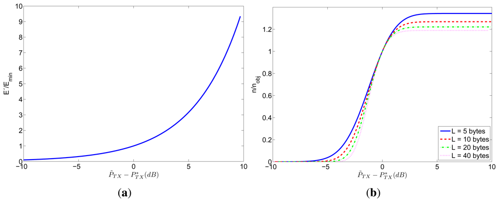
Figure 4 shows how the errors in the transmission power affect the consumed energy and the number of received packets. In particular, Figure 4(a) represents the ratio between the energy consumption E′ corresponding to the estimated transmission power P TX ′ and E_min (corresponding to the optimum transmission power P TX ∗) as a function of the error in the transmission power ( P TX ′ − P TX ∗ ). This relation is valid for any value of n_obj, for any W/v_b ratio for any packet length l and for any distance between transmitter and receiver. On the other hand, Figure 4(b) shows the relation between the number of received packets n corresponding to the estimated transmission power P TX ′ and the desired number of received packets n_obj (corresponding to the optimum transmission power P TX ∗) as a function of the error in the transmission power. This relation is valid for any value of n_obj, for any W/v_b ratio and for any distance between transmitter and receiver, but depends on the packet length l.

As shown in Figure 4(a), the consumed energy E′ will be greater than the minimum value (E_min) if the transmission power is overestimated. Furthermore, the relation between the error in the transmission power ( P ∼ TX − P TX ∗ ) and the corresponding energy consumption is exponential. For example, if the transmission power is overestimated in 1 dB the energy consumption will be a 26% higher than E_min, if it is overestimated in 2 dB the energy consumption will be a 59% higher than E_min, and if it is overestimated in 3 dB the energy consumption will be doubled with respect to E_min. On the other hand, as shown in Figure 4(b), the number of received packets n will be lower than the desired n_obj if the transmission power is underestimated. Notice that the behavior is quite sharp, especially for longer packets. For example, for 40-bytes packets, if the transmission power is underestimated in only 1.4 dB, the number of received packets will be halved with respect to the objective n_obj, and if the transmission power is underestimated in more than 4 dB, the number of received packets will be practically zero.

The behavior shown in these figures is valid for both TOA-based and RSS-based localization schemes, but as the probability distribution of the distance estimation is different for the two localization schemes (see Appendix A and B), the probability distribution of P ∼ TX − P TX ∗ will also be different. Therefore, the frequency of underestimations and overestimations of the transmission power will depend on the distance estimation method, and this will affect the probability distribution of the energy consumption and the number of received packets, as we will see next.

This error in the transmission power can be calculated as: (17) P TX ′ − P TX ∗ ( d B ) = 10 η log d ∼ dwhere d̃ is the estimated distance. Appendix A and B derive the expressions of d̃ for TOA-based and RSS-based localization respectively. In a TOA-based localization scheme the distance estimation is given by Equation (24), therefore the difference between calculated and optimum transmission power will be given by: (18) P TX ′ − P TX ∗ = 10 η log d + 𝒩 ( 0 , σ ) d = 10 η log 𝒩 ( 1 , σ / d )where σ = c ⋅ σ t / n or σ = c ⋅ σ t / 2 n, as explained in Appendix A. On the other hand, in a RSS-based localization scheme the distance estimation is given by Equation (28), thus the difference between calculated and optimum transmission power will be given by: (19) P TX ′ − P TX ∗ = 𝒩 ( 0 , σ )with σ = σ RSS / n.

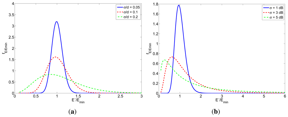
Figure 5 shows the probability density function of the relative energy consumption (E′/E_min) for the cases of TOA-based and RSS-based localization. The different curves correspond to different values of σ/d and σ respectively. Notice that in the TOA case the individual values of σ and d do not have any influence, as long as the relation σ/d remains the same. This can be easily understand from Equation (18). In both cases, the probability of consuming more energy increases with σ. Furthermore, the mean value of E′/E_min also increases when the standard deviation increases.

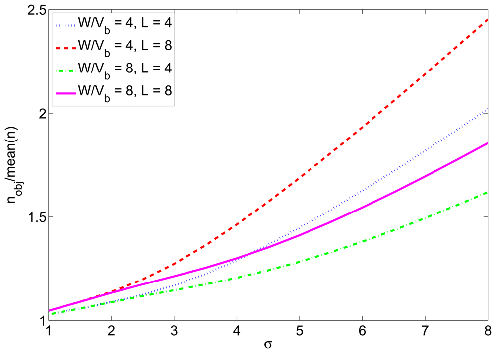
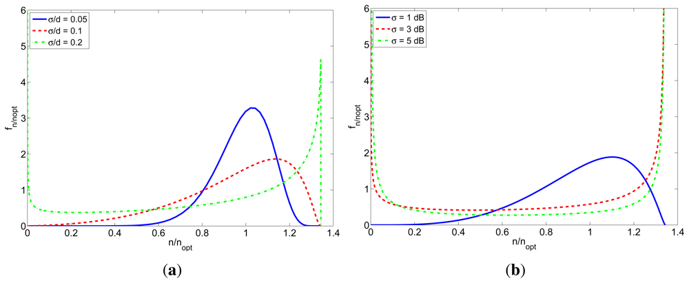
Figure 6 shows the probability density function of the relative number of received packets (n/n_obj) for TOA-based and RSS-based localization. The different curves correspond to different values of σ/d and σ respectively, and were calculated for a packet length of l = 5 bytes (different packet lengths produce similar results, but a little more sharper as the packet length increases). In both cases, when the standard deviation is bigger, the probability of not receiving the desired number of packets is higher. It can be also seen that if the standard deviation is over a certain threshold, the pdf begins to be bimodal. This is because the margin of SNR for which the PRP takes intermediate values is small, so if the standard deviation is big enough, the probability of receiving packets with a very low or very high SNR (enough to make PRP = 0 or PRP = 1 respectively) is significant.

In conclusion, for both TOA and RSS-based localization methods, a greater variance in the measurements will produce a greater variance in the optimum transmission power estimation and thus, more energy consumption and a higher probability of losing packets.

The proposed strategy has been derived from the assumption that the power consumption of the transmitter is equal to the transmitted power. However, for real devices, this assumption may not be true due to the inefficiencies of the hardware. In this case, the theoretical strategy previously proposed has to be slightly modified, by substituting the transmission power p_tx in Equation (5) by the power consumption at transmission p_T, which in general may depend on the transmission power in a non-linear way. Therefore, the real energy consumption is related to the ideal one, given by Equation (5), by the following expression: (20) E real = E TX ⋅ p T p tx = E TX ⋅ g ( p tx )where g(p_tx) = p_T/p_tx is a nonlinear function of p_tx that will be different for each type of hardware.

Similarly to the ideal case, we can minimize this energy consumption with respect to the snr by setting the derivative equal to zero (and working with the mean values of the random variables). After some algebraic calculations, we finally obtain the following expression: (21) ∂ E real ∂ snr | x = x ∗ = 0 ⇒ g ( p tx ) ⋅ ( 2 − 8 l x ⋅ e − x 2 2 ( 1 − Q ( x ) ) ⋅ 2 π ) + v b W ⋅ x 2 ⋅ ∂ g ( p tx ) ∂ p tx ⋅ d η n rx a ⋅ e 1 2 ( σ ⋅ ln 10 10 ) 2 = 0

The value of x (and therefore, the value of snr) for which this expression is equal to 0 gives the minimum average energy consumption. Clearly, the result will depend on the hardware characteristics.

As an illustration, we next apply this method for two common radio chips used in wireless sensor networks devices: the ChipCon chips CC1000 and CC2420. Clearly, real devices also include other components apart from the radio chip, which will also affect the energy consumption. However, this example illustrates how to proceed in a general case where there is a nonlinear relationship between transmission power and consumption. Several values of p_T as a function of p_tx can be obtained from the datasheets of the two chips [30,31]. In order to have an approximate expression of g(p_tx) and its derivative, we approximated these sets of points by an analytical expression of the form g ( p tx ) = U ⋅ p tx V. Table 1 shows the values of U and V for the two chips and the correlation coefficient of the fitting. As it can be seen, there is a high correlation in both cases, which means that the considered expression fits well to the data.

Introducing this expression and its derivative in Equation (21), and after some algebraic manipulation, we finally obtain that the value of x for which the average energy consumption reaches a minimum (x*) satisfies the following expression: (22) x ∗ e − x ∗ 2 / 2 ( 1 − Q ( x ∗ ) ) = 2 π 4 l ⋅ ( 1 + V )

Thus, if we manage to achieve at the receiver the corresponding value of signal to noise ratio snr* (using Equation (8)), the real energy consumption will be minimized. Similarly to the ideal case, the optimum value of the snr at the receiver to achieve the lowest energy consumption does not depend on the accuracy we want to obtain or on the propagation characteristics, it only depends on the packet length l and on the W/v_b ratio, i.e., its value is constant for a given network and does not need to be calculated in real time. Again, as in the ideal case, there is an optimum value of T corresponding to snr*, which can be calculated from Equation (11). Finally, the corrections for the transmission power and the packet transmission rate can be calculated similarly to the ideal case.

In conclusion, the general receipt to apply the proposed method for a specific device is:

Characterize the energy consumption of the device as a function of the transmission power

In order to simulate a realistic situation, we carried out some experiments to characterize the propagation environment of our laboratory using Memsic's MICAz motes [32]. The objective was to check that the models proposed in Section 3 approximately reflect the behavior of our wireless network and, at the same time, to extract the values of some of the model parameters that we need for the simulations.

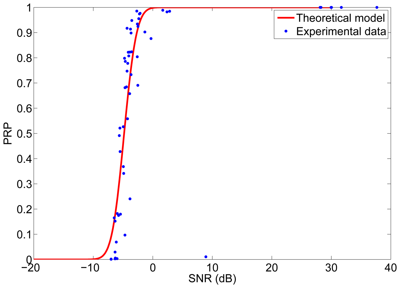
The first set of experiments were carried out to determine the PRP as a function of the snr. These experiments were made with Memsic's MICAz motes. The MICAz is a 2.4 GHz mote with direct sequence spread spectrum radio, which uses an O-QPSK modulation scheme. Two motes were used for the experiments, one as transmitter and one as receiver. The experiments were carried out in a laboratory environment in which there were obstacles and people sitting or walking and interfering signals from other motes and other wireless systems working at the same frequency (WiFi). In each experiment, the transmitter node transmitted a packet of 8 bytes every second and the receiver node measured the RSS of the received packets, from which we obtained the snr at the receiver. The experiment was repeated for different distances between transmitter and receiver and for different transmission powers in order to have different values of snr at the receiver. The experimental results are shown in Figure 7, together with the theoretical model given by Equation (1). As it can be noticed in Figure 7, the experimental data adjust quite well to the model, with the exception of some outliers. From this experiment we obtained a value of N_RX = −87 dBm for the noise level at the receiver.

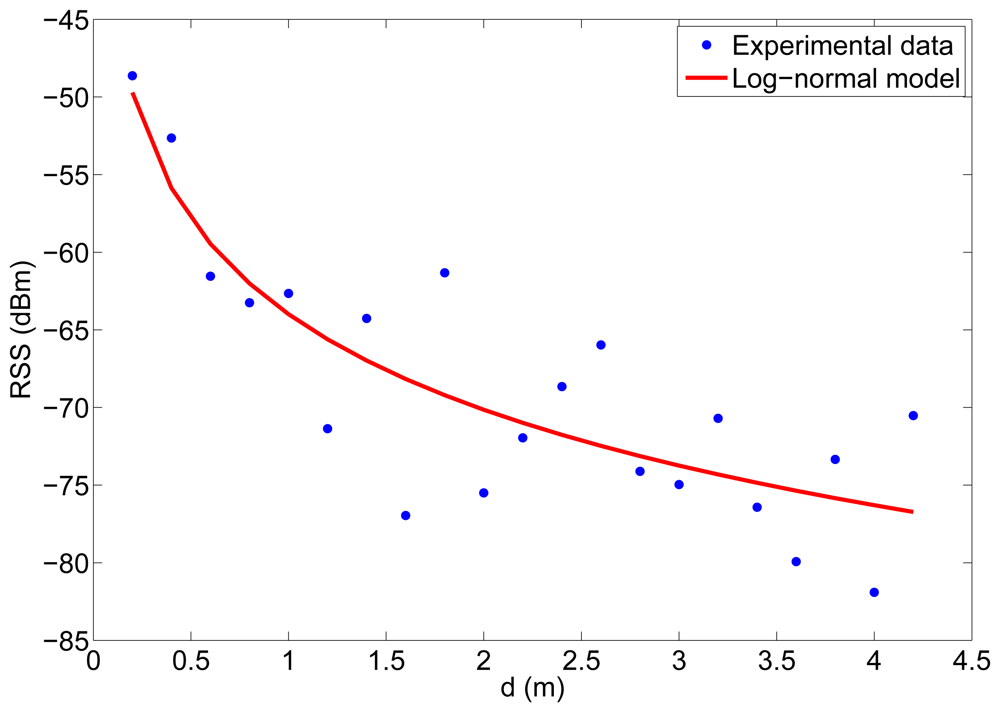
We also made some experiments to characterize our radio channel, that is, to establish a relation between transmission and received power in terms of the distance. In these experiments, two MICAz motes were used again, with the same configuration as in the PRP experiments, and the tests were carried out in different rooms. The RSS of the received packets was measured for different distances between transmitter and receiver. At each position, several measurements of RSS were obtained, in order to average their values. In these experiments the transmitter used P_TX = 0 dBm. The results from one of the experiments are shown in Figure 8. The curve in Figure 8 represents the fitting of the mean of Equation (2) to these experimental data and was calculated using the Levenberg–Marquardt algorithm, taking d₀ = 1 m, P_TX = 0 dBm and η and A as free parameters. From this experiment we obtained a value for the path loss exponent and the constant A (η = 2 and A = −64 dB). For other experiments, the estimated values of A were between −60 dB and −70 dB and the estimated values of η were between 2 and 3.

We have run a set of simulations to evaluate the energy consumption of the proposed strategy in several scenarios. In these simulations, the performance of the proposed strategy is also compared with other two strategies: (1) sending n packets with the highest transmission power available by hardware and (2) sending n packets with a transmission power that depends on the estimated inter-node distance: P_TX(dBm) = −A + 10η logd̃/d₀ + N_RX(dBm), which is the most common strategy when power adaptation is used (note that this is equivalent to using a transmission power such that the SNR at the receiver is 0 dB).

In these simulations, we considered networks composed of reference nodes and mobile nodes. In order to estimate the position of the mobile nodes, each reference node transmits packets to them. These nodes measure the RSS of the received packets and calculate their distance to each of the reference nodes. With these range estimations and the known positions of the reference nodes, the mobile nodes are able to calculate their own positions. As soon as they have an estimated value of their physical position, they can send packets to other nodes with the information about their estimated position and act themselves as reference nodes. Consequently, every node of the network will transmit packets to and receive packets from every other node within its communications range. Considering the transmission strategy proposed in the previous section for a single link, we applied it to the whole network by finding at each node the optimum transmission strategy ( P TX ∗ and T ∗ ) for its furthest neighbor (closer neighbors will be guaranteed to receive at least the same average number of packets). The transmission power P_TX is adaptively modified, by estimating from Equation (3) the value necessary to achieve the desired SNR* at the furthest neighbor. As an estimate of the distance between the transmitter and its furthest neighbor is needed, the method is refined iteratively: first, the transmission power is set to an initial (high) value and a preliminary distance estimation is obtained; then, the transmission power is modified according to the distance estimation.

First, we simulated a network composed of four reference nodes deployed randomly in a 15 × 15 m² room and one mobile node that stays in the center of the room during 20 seconds. The localization is done every second (T₀ = 1 s) and the desired accuracy is such that n = 5. The communication channel was simulated using the log-normal model in Equation (2) with A = −65 dB, η = 2.5, d₀ = 1 m and σ = 0 dB (ideal channel without shadowing). Packet reception was modeled with Equation (1), using W = 2 Mhz and v_b = 250 kbps. The average energy consumption of 5000 simulations (50 different node placements, 100 simulations for each placement), which stays constant after the first localization interval, is shown in Table 2 for different values of the packet length. On the other hand, in this ideal simulation environment, the three strategies guarantee that the average number of received packets is n = 5 at the furthest node during the whole simulation. It can be seen that the proposed strategy gives the lowest energy consumption (about 47% the energy consumption of strategy #2 for l = 4) and, at the same time, guarantees that the average number of received packets is n = 5 at the furthest node. The length of the localization packets also has an influence in the energy consumption: the gain of the proposed method with respect to the other two is higher for lower values of l.

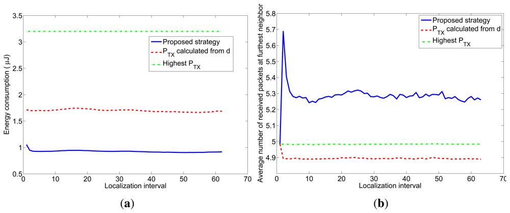
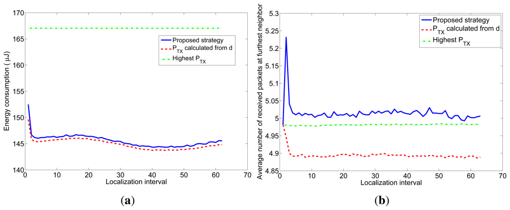
Next, to simulate a more realistic scenario, we added shadowing with σ = 2 dB and node movement to the previous simulation. We simulated a 7m-radius circular trajectory centered in the simulated area. The influence of the shadowing is twofold, as explained in Section 4.2. On one hand, the distances are usually underestimated, so the transmission power calculated from them to reach the receiver with the desired snr has to be corrected with the correction margin given at Figure 2. On the other hand, even when the optimum transmission power is used, the final snr at the receiver may not be the desired one due to the effects of shadowing. To counteract this effect, we have corrected the number of transmitted packets with the factor given at Figure 3. The average results of 5000 simulations are shown in Figure 9. Figure 9(a) shows the average energy consumption of the three strategies for each localization interval and Figure 9(b) shows the average number of received packets at the furthest node. It can be seen that the proposed strategy gives the lowest energy consumption (about 54% the energy consumption of strategy #2) and, at the same time, guarantees that, at least, the average number of received packets at the furthest node is n = 5. These results were obtained for localization packets of length l = 4 bytes. Table 3 shows the energy consumption of the proposed strategy for other values of l and Table 4 shows the average number of received packets at the furthest neighbor. It can be seen that the length of the localization packets has an effect on the performance of the proposed strategy: the longer the packet is, the lower is the gain in energy consumption with respect to other strategies. This is because when l increases, the optimum snr increases as well and gets closer to 1 (SNR = 0 dB), so the difference in energy consumption with respect to strategy #2 decreases. In any case, the proposed strategy always assures a given number of received packets, in contrast to strategy #2 and, moreover, entails energy savings with respect to other strategies.

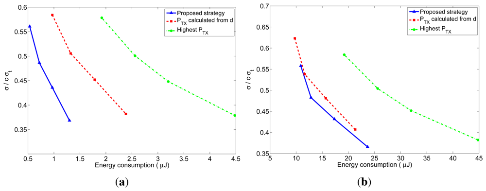
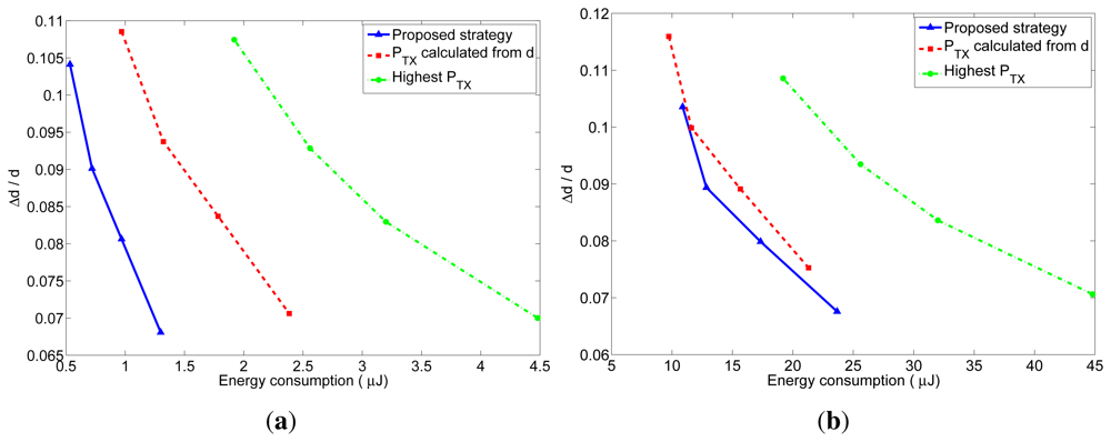
As explained before, the number of received packets at the furthest neighbor determines the accuracy of the distance estimation at these nodes. The accuracy of the distance estimations in closer neighbors will be at least as good as the one at the furthest neighbor. In order to better understand the behavior of the proposed transmission strategy, we have represented in Figures 10 and 11 the relation between the average energy consumption and the accuracy of the distance estimations for TOA and RSS measurements respectively, obtained from the previous realistic simulations for different values of n. The x-axis represents the average energy consumption of the whole network at each localization interval, which was calculated by summing up the energy consumption of all the nodes at each localization interval, and averaging the result over time (excluding the first localization intervals, in order to eliminate the initialization effects) and over the 5000 simulations. The y-axis represents the distance estimation accuracy at the furthest neighbor, which was calculated from the average number of received packets at the furthest neighbors. This value was obtained by taking, at each localization interval, the furthest neighbor for each node of the network, and averaging the number of packets received by these nodes. Then the results were averaged over time (excluding the first localization intervals) and over the 5000 simulations. From the number of received packets, the accuracy of the distance estimation was calculated according to the expressions of the TOA-based and RSS-based distance estimations which are derived in Appendix A and B. In the TOA case, the estimated distance is a Gaussian random variable given by Equation (24) with mean equal to the real distance and standard deviation given by Equation (25) for one-way TOA measurements or by Equation (26) for two-way TOA measurements. Figure 10 represents the accuracy as the ratio between the standard deviation of the distance estimation (σ) and the factor c · σ_t, which is the standard deviation corresponding to one one-way TOA measurement. Therefore, the accuracy in this figure should be read as relative to the accuracy of one TOA measurement. In the RSS case, the estimated distance is a log-normal random variable with variance given by Equation (32). Figure 11 represents the accuracy as the ratio between the standard deviation of the distance estimation (Δd) and the real distance d, where the distance estimation variance was calculated for a channel with σ_RSS = 2 dB (for other values of σ_RSS the particular values of the relative accuracy change: they get bigger for bigger values of σ_RSS, but the relation between the three strategies remains the same). Therefore, the accuracy in this figure should be read as a relative error in the distance (a percentage of the real distance). From these figures, it can be clearly noticed that the proposed method has a better performance regarding both the energy consumption and the accuracy of the distance estimations. The gain with respect to the other strategies is especially noticeable for short localization packets, which is the usual situation, as these packets do not carry any data information.

Finally, we have evaluated the performance of the proposed strategy for a case in which the power consumption is not equal to the transmitted power (which is usually the case for real devices). To this end, we repeated the previous simulation experiments considering the energy model for the CC2420 radio chip described in Section 4.4 and following the steps described in that section to adjust the proposed strategy. Figure 12 shows the results for n = 5 and l = 4 bytes.

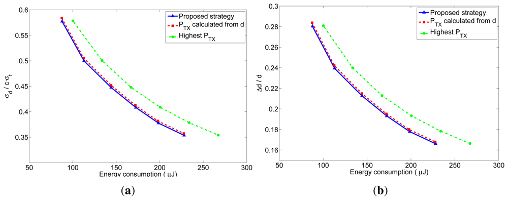
It can be seen in Figure 12(b) that the proposed strategy is again the only one that guarantees the desired accuracy (n = 5), but in this case its energy consumption (Figure 12(a)) is a little bit higher than for strategy #2 (which does not guarantee the desired accuracy). To better understand this behavior, we show in Figure 13 the relation between the average energy consumption and the accuracy of the distance estimations for the different strategies.

As it can be noticed, for a given energy consumption, the proposed strategy achieves better accuracy than strategy #2, and for a given accuracy, the proposed strategy has lower energy consumption. Our proposed method shows still a gain, but of lower entity with respect to the ideal case shown in Figures 10 and 11. The reason is that for this particular hardware, the optimum value of the SNR is closer to 0 dBm, thus, there is not a big margin for improvements, as strategy #2 is practically a strategy that tries to achieve a SNR = 0 dBm at the receiver.

To sum up, the proposed strategy always guarantees a desired accuracy in the distance estimation and, at the same time, yields energy savings, especially when the optimum value of the SNR is low. As this optimum value depends on the particular energy consumption characteristics of the wireless device, bigger savings are expected for devices with more similar characteristics to that of the ideal case.

References

- Stojmenovic, I. Position-based routing in ad hoc networks. IEEE Commun. Mag. 2002, 40, 128–134. [Google Scholar]
- Zhang, J.; Yu, J.-P.; Zhou, S.-W.; Lin, Y.-P.; Li, G. A survey on position-based routing algorithms in wireless sensor networks. Algorithms 2009, 2, 158–182. [Google Scholar]
- Pattem, S.; Krishnamachari, B.; Govindan, R. The impact of spatial correlation on routing with compression in wireless sensor networks. ACM Trans. Sens. Netw. 2008, 4, 24. [Google Scholar]
- Tarrío, P.; Valenzise, G.; Shen, G.; Ortega, A. Distributed Network Configuration for Wavelet-Based Compression in Sensor Networks. Proceedings of the 3rd International Conference on GeoSensor Networks, GSN '09, Oxford, UK, 13–14 July 2009; volume 5659. pp. 1–10.
- Gezici, S. A survey on wireless position estimation. Wirel. Pers. Commun. 2008, 44, 263–282. [Google Scholar]
- Tarrío, P.; Bernardos, A.; Casar, J. Weighted least squares techniques for improved received signal strength based localization. Sensors 2011, 11, 8569–8592. [Google Scholar]
- Lorincz, K.; Welsh, M. MoteTrack: A robust, decentralized approach to RF-based location tracking. Pers. Ubiquitous Comput. 2007, 11, 489–503. [Google Scholar]
- Yin, J.; Yang, Q.; Ni, L. Learning adaptive temporal radio maps for signal-strength-based location estimation. IEEE Trans. Mobile Comput. 2008, 7, 869–883. [Google Scholar]
- Yick, J.; Mukherjee, B.; Ghosal, D. Wireless sensor network survey. Comput. Netw. 2008, 52, 2292–2330. [Google Scholar]
- Karalar, T.; Yamashita, S.; Sheets, M.; Rabaey, J. A Low Power Localization Architecture and System for Wireless Sensor Networks. Proceedings of the IEEE Workshop on Signal Processing Systems, Austin, TX, USA, 13–15 October 2004; pp. 89–94.
- Anastasi, G.; Conti, M.; Di Francesco, M.; Passarella, A. Energy conservation in wireless sensor networks: A survey. Ad Hoc Netw. 2009, 7, 537–568. [Google Scholar]
- Raghunathan, V.; Schurgers, C.; Park, S.; Srivastava, M. Energy-aware wireless microsensor networks. IEEE Signal Process. Mag. 2002, 19, 40–50. [Google Scholar]
- Reichenbach, F.; Salzmann, J.; Timmermann, D.; Born, A.; Bill, R. DLS: A Resource-Aware Localization Algorithm with High Precision in Large Wireless Sensor Networks. Proceedings of the 4th Workshop on Positioning, Navigation and Communication, Hannover, Germany, 22 March 2007; pp. 247–254.
- Born, A.; Bill, R. Reducing the Calculation for Precise Localization in Wireless Sensor Networks. Proceedings of the IEEE 71st Vehicular Technology Conference, Taipei, Taiwan, 16–19 May 2010; pp. 1–5.
- Xu, Y.; Winter, J.; Lee, W. Prediction-based Strategies for Energy Saving in Object Tracking Sensor Networks. Proceedings of the IEEE International Conference on Mobile Data Management, Berkeley, CA, USA, 19–22 January 2004; pp. 346–357.
- Tilak, S.; Kolar, V.; Abu-ghazaleh, N.; Kang, K. Dynamic Localization Control for Mobile Sensor Networks. Proceedings of the 24th IEEE International Performance, Computing, and Communications Conference, Phoenix, AZ, USA, 7–9 April 2005; pp. 587–592.
- Lin, T.; Huang, P.; Chu, H.; You, C. Energy-efficient boundary detection for RF-based localization systems. IEEE Trans. Mobile Comput. 2009, 8, 29–40. [Google Scholar]
- You, C.; Chen, Y.; Chiang, J.; Huang, P.; Chu, H.; Lau, S. Sensor-enhanced Mobility Prediction for Energy-efficient Localization. Proceedings of the Third Annual IEEE Communications Society Conference on Sensor, Mesh and Ad Hoc Communications and Networks, Reston, WV, USA, 25–28 September 2006; pp. 565–574.
- Pandey, S.; Prasad, P.; Sinha, P.; Agrawal, P. Localization of Sensor Networks Considering Energy Accuracy Tradeoffs. Proceedings of the International Conference on Collaborative Computing: Networking, Applications and Worksharing, San Jose, CA, USA, 19–21 December 2005; p. 10.
- Tarrío, P.; Bernardos, A.; Casar, J. A Transmission Rate and Energy Design for Power Aware Localization in Ad Hoc and Sensor Networks. Proceedings of the IEEE 18th International Symposium on Personal, Indoor and Mobile Radio Communications, Athens, Greece, 3–7 September 2007; pp. 1–5.
- Tarrío, P.; Bernardos, A.; Casar, J.; Besada, J. Design and Accuracy Analysis of a Power-efficient TOA-based Location Scheme for Wireless Networks. Proceedings of the 7th International Workshop on Applications and Services in Wireless Networks, Santander, Spain, 24–25 May 2007; pp. 55–62.
- Tarrío, P.; Bernardos, A.; Casar, J. An Optimal Strategy for Power Sensitive Localization in Ad Hoc Networks. Proceedings of the 4th International Symposium on Wireless Communication Systems, Trondheim, Norway, 16–19 October 2007; pp. 143–147.
- Patwari, N.; Ash, J.; Kyperountas, S.; Hero, A., III; Moses, R.; Correal, N. Locating the nodes: Cooperative localization in wireless sensor networks. IEEE Signal Process. Mag. 2005, 22, 54–69. [Google Scholar]
- Proakis, J.; Salehi, M. Digital Communications; McGraw-Hill: New York, NY, USA, 1995. [Google Scholar]
- Cerpa, A.; Wong, J.; Kuang, L.; Potkonjak, M.; Estrin, D. Statistical Model of Lossy Links in Wireless Sensor Networks. Proceedings of the Fourth International Symposium on Information Processing in Sensor Networks, Los Angeles, CA, USA, 25–27 April 2005; pp. 81–88.
- Sarkar, T.; Ji, Z.; Kim, K.; Medouri, A.; Salazar-Palma, M. A survey of various propagation models for mobile communication. IEEE Antennas Propagn. Mag. 2003, 45, 51–82. [Google Scholar]
- Rappaport, T. Wireless Communications: Principles and Practice; Prentice Hall PTR: Upper Saddle River, NJ, USA, 2001. [Google Scholar]
- Moravek, P.; Komosny, D.; Simek, M.; Jelinek, M.; Girbau, D.; Lazaro, A. Signal Propagation and Distance Estimation in Wireless Sensor Networks. Proceedings of 33rd International Conference on Telecommunications and Signal Processing Conference, Baden, Austria, 17–20 August 2010.
- Martín, H.; Tarrío, P.; Casar, J. Reducing Positioning Errors Through Space Averaging for Location Based Indoor Applications. Proceedings of the Workshop on User-Centric Technologies and Applications, Salamanca, Spain, 12 November 2007; pp. 59–67.
- 2012. Available online: http://www.astlab.hu/pdfs/cc1000.pdf (accessed on 31 October 2012).
- 2012. Available online: http://inst.eecs.berkeley.edu/∼cs150/Documents/CC2420.pdf (accessed on 31 October 2012).
- Memsic Sensor Motes Specifications. 2012. Available online: http://www.memsic.com/products/wireless-sensor-networks/wireless-modules.htm (accessed on 31 October 2012).
- Law, A.; Kelton, W. Simulation, Modelling and Analysis; McGraw-Hill International Series: New York, NY, USA, 2000. [Google Scholar]