Static shadows give us clues about the scene represented in an image or a video sequence, including the shape, the objects, and the relative position of the light sources [23]. Additionally, these shadows seem to modify the perceived shape and color of the objects [24]. Some methods have exploited the color properties of objects as they are affected by shadows. For instance, Nagao et al. [11] and Scanlan [25] used histogram analysis to detect shadows. On the other hand, Jiang and Ward [26] reported a method for identifying and classifying shadows in real images based on the constraints that shadows possess in both intensity and geometry. Suzuki et al. [27] proposed a compensation method to remove shadows in aerial images transforming the red, green, and blue (RGB) values of the original image into hue, saturation and intensity (HSI) values. Some other researchers have exploited the relationship between the different homogeneous color regions in an image. This allows them to obtain first the edges of a shadow and then extract the shadow area. In addition, several color spaces have been explored in order to detect shadows, e.g., normalized red, green, and blue (rgb), hue (H) and saturation (S), c1c2c3 and l1l2l3 [28]. Finlayson et al. [29] proposed a method to process a 3-band color image to remove the shadows based on edge information. Moreover, Gevers and Stokman [30] also used color information to classify edges based on whether the transition between regions is due to shadows, abrupt surface orientation changes, illumination, or material changes. Levine and Bhattacharyya [31] developed a strategy that does not require camera calibration or other a priori information regarding the scene.

Unlike static shadows, the moving ones are associated with dynamic objects. In many situations, moving objects and their shadows are detected as one single region. The above effect may require a stage to separate the object from its cast shadows, like the one described in the method proposed by Sonoda and Ogata [32], which is based on projective geometry. In addition, other authors proposed different strategies to detect moving shadows based on the use of diverse color models. For example, Horprasert et al. [33] used a brightness and chromaticity color model. Moreover, Mikic et al. [34] used a method that combines different color spaces. The authors considered three features at each pixel: brightness, normalized red and normalized blue. In this method, each feature is analyzed by a posterior probability estimator that computes probabilities for three classes: background, foreground and shadows. Nadimi and Bhanu [35] proposed an algorithm to detect moving shadows in outdoor environments based on a spatio-temporal albedo test and a dichromatic reflection model. In addition to the color spaces, some shadow features such as transparency (a shadow always darkens the region upon which it falls) and homogeneity (the relationship between pixels under shadows is roughly linear) have been used to detect moving shadows in outdoor traffic scenes [36]. However, this method considers a linear relationship between shadow and non-shadow regions and only gray-scale images are processed. On the contrary, Cucchiara et al. [37] developed a method for segmenting moving objects without their shadows by using color information. This algorithm transformed the original input image from RGB color space to hue, saturation, and value (HSV). Recently, Sanin et al. [15] presented a survey of several techniques for moving cast shadow detection. It is important to understand that the strategies these authors compared cannot be applied to the problem that we describe, because these techniques first detect changes in the scene (moving objects) and then classify the detected pixels as foreground (object) or shadow. Under the above assumption, the shadows cast by static objects will be part of the background; or, if a large enough interval of time is selected to perceive changes in the shape and position of the shadows cast by static objects, the moving shadow detection strategies will detect only the parts of the shadow that change, which is typically the region around the boundaries.

A serious limitation in the systematic evaluation of algorithms to detect shadows cast by static objects during extended periods of time is the lack of a standard data set with annotated ground truth. Based on this fact, we used two synthetic sequences that simulate the changes in the sun's position over a long period of time (days) for a particular geographical position. The advantage of using synthetic images is that the ground truth is automatically generated.

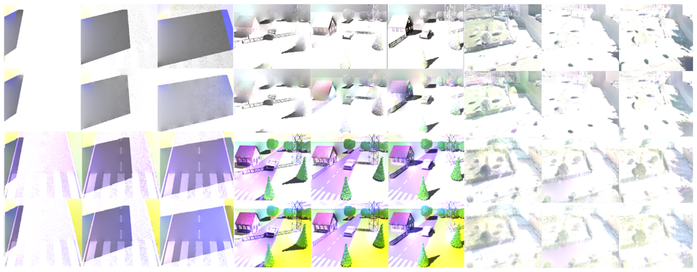
The synthetic sequences were rendered using the POV-Ray software [38]. We designed the first synthetic sequence in accordance to the one introduced by Masushita et al. in [20], to analyze the problem of the computation of intrinsic images. This data set has 20 frames with a resolution of 512 × 384 pixels (width × height). It represents white lines on a road surface (see first, second and third columns in Figure 2). The shadow effect was created using a rectangular object out of the field of view of the camera, changing the light source positions on the horizontal axis. The second synthetic sequence simulates the sun position over 12 consecutive days. We generated 40 frames per day with a resolution of 512 × 384 pixels (width × height). We designed this data set considering objects that exist in a typical outdoor location. We included in our scenario static objects such as buildings, a road, trees, and bushes, among others (see fourth, fifth and sixth columns in Figure 2).

In the synthetic sequences, the shadow effect was created using the following procedures. First, we computed the sun position in a given geographical location. We used an off-the-shelf Geographical Positioning System (GPS) to obtain the latitude, longitude, and elevation of a camera installed in the real outdoors scenario. Then, using the algorithm presented by Reda and Andreas [41] the sun position (elevation and azimuth angles at a given location) as a function of the local time and position of the observer was computed from dawn to dusk during twelve consecutive days. After that, the values of the elevation and azimuth angles were transformed to Cartesian coordinates for the rendering software to simulate the changes in the sun position.

In addition to the synthetic sequences, we recorded a real data set. For this purpose, we positioned a fixed camera on the roof of a building and took images from dawn to dusk during seven consecutive days (see seventh, eighth, and ninth columns in Figure 2). The camera was fixed to capture a motionless area, to facilitate the analysis of shadows cast by static objects during this long time interval. Each image has a resolution of 1,032 × 776 pixels (width × height). We selected the location, based on the challenge that it represents for the detection of shadows cast by static objects. In the scenario, there are regions that are shaded during all daylight and others with huge shadows. Additionally, some shadows have significant changes in the intensity, up to the point that it is difficult to define the boundaries. This data set also has isolated shadows cast by trees and shadows mixed that are cast by several objects. Another important feature of the data set is that only small fast traveling clouds appear in the sequence, resulting in the presence of shadows during all daylight.

The concept of intrinsic images was introduced by Barrow and Tenenbaum [18]. It describes an image decomposition in terms of characteristics such as range, orientation, reflectance, and incident illumination. One of the simplest models is described by the product I(x, t) = R(x, t)L(x, t), where I(x, t) is an image, x is a pixel index, and t represents the frame index respect to time. The reflectance image R(x, t) represents the properties of the object to reflect light in the direction of the pixel x. The illumination L(x, t) describes the distribution of the incident light and accounts for some of the shading effects and shadows. Deriving this decomposition is a fundamentally ill-posed problem [42]. Weiss shows that this problem can be solved if one considers the reflectance to be constant while the illumination varies [19]. Matsushita et al. [20] extended Weiss' method to handle scenes where the Lambertian assumption does not hold. They consider that both the illumination and reflectance may change. In their method, they analyze the magnitude of the gradient in the reflectance component. If the magnitude in a given position is larger than a given threshold, the illumination values at that position are removed and added to the reflectance image. As a result, for each input image two others are obtained, one for the reflectance and another for the illumination. Although with this method a reflectance component is obtained representing the texture in the scene, some texture appears in the illumination image even for different values of the threshold. Another strategy to derive intrinsic images was introduced by Land and McCann [39]. They proposed the Retinex theory, which expresses that the reflectance component can be separated from the illumination if the later is assumed to vary slowly. An extension which uses color have been introduced by Finlayson [8,40]. In a different approach, a learning-based method to separate reflectance and illuminate was proposed by Tappen et al. [42]. They successfully separated the reflectance and the illumination components for a light source in a synthetic data set. In 2009, Grosse et al. [22] introduced an intrinsic image model with three terms: reflectance, illumination, and specularity C(x, t). All together, this decomposition is expressed as: I(x, t) = R(x, t)L(x, t) + C(x, t). Nonetheless, in this model, the problem of factoring the information between reflectance and illumination remains.

Weiss [19] proposed that intrinsic components can be derived by using a sequence of images without motion acquired with a fixed camera in an outdoor scene under varying illumination conditions. This method uses the statistics of natural images [43] and assumes that illumination images will give rise to sparse filter outputs. Then, the scene reflectance image is obtained by taking the median of the filtered image sequence in the log domain. Additionally, the method assumes that the scene is Lambertian and the fact that illumination images have less contrast than reflectance images.

Weiss uses the following equation to derive intrinsic images: (1) { I ( x , t ) } t = 1 T = R ( x ) { L ( x , t ) } t = 1 T

For convenience, Weiss worked in the log domain. In what follows, we will represent variables in the log domain using lower-case letters, e.g., i(x, t) to represent the logarithm of I(x, t). According to Weiss' method, a reflectance edge image is computed by taking the median along the time axis of the convolution between the derivative filter and a given image: (2) r ( x ) = median [ f m ∗ i ( x , t ) ]where r(x) is the constant edge reflectance image and f_m represents the derivative niters f₀ = [0, 1, −1] or f₁ = [0, 1, −1]^T. Then, the illumination edge images l(x, t) are computed subtracting the edge maps of the input and the reflectance images: (3) l ( x , t ) = i ( x , t ) − r ( x )

Matsushita et al. [20] analyzed the reflectance component based on the strategy proposed by Weiss and the derived time variable of reflectance and illumination images. They noticed that in real-world scenes, the Lambertian assumption is not sufficient to derive intrinsic images. Matsushita et al. analyzed the magnitude of the gradient of the reflectance edge image r(x) by assuming that texture information should not be present. Then, if the magnitude of the gradient in a given position of the reflectance image is larger than a given threshold T, the texture edge is removed from the illumination image l(x, t) and added to the time-varying reflectance image denote by (4) r ( x , t ) = { r ( x ) + l ( x , t ) if | r ( x ) | > T r ( x ) otherwise and (5) l ( x , t ) = { 0 if | r ( x ) | > T l ( x , t ) otherwise

After the time-varying reflectance and illumination component edge maps are obtained, a deconvolution process is applied to get a reconstructed image, as (6) < r ^ , l ^ > = g ∗ ( ∑ m f m ′ < r , l > )where r̂ and l̂ are the reflectance and illumination time-varying reconstructed images, f m ′ is the inverse filter of f_m, and g is the filter which satisfies the equation: (7) g ∗ ( ∑ m f m ′ ∗ f m ) = δ

The Retinex algorithm, proposed in [39], analyzes logarithm image gradients. This method considers that small gradients are due to changes in the illumination, while large gradients represent texture. The threshold value that classifies the edges into reflectance or illumination is defined for the horizontal i_x(x, t) and vertical i_y(x, t) derivatives. This method can be applied to gray-scale images or each color band separately. The formal description for gray-scale images is: (8) r k ( x , t ) = { i k ( x , t ) if | i k ( x , t ) | > T 0 otherwisewhere k can be either x or y.

An extension of the Retinex algorithm to color images has been proposed by Finlayson et al. [40]. This method analyzes logarithm image gradients in color space. Here, two thresholds are considered, one for the chromaticity T_C and another for the brightness T_B subspace, as (9) r k ( x , t ) = { i k B ( x , t ) if | i k B ( x , t ) | > T B i k C ( x , t ) if | i k C ( x , t ) | > T C 0 otherwisewhere k can be either x or y.

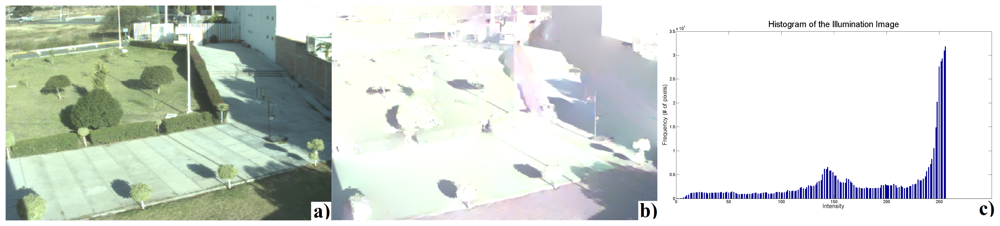
None of the methods described earlier was designed to estimate the position of the shadows. However, the illumination component, l(x, t), encodes information about shadows, S(x, t). So to compare their usefulness for shadow detection, we devised a method based on thresholding the illumination histogram. Figure 3 illustrates an example of the original image, where illumination and its corresponding histogram are estimated with the method proposed by Matsushita et al. Then, each pixel of the illumination image is classified into shadow (C1) or non-shadow (C2). For this purpose, an experimental threshold (T) is selected and the shadow segmentation process is achieved, as (10) S ( x , t ) = { C 1 if l ( x , t ) < T C 2 otherwise

We used the same procedure to detect shadows in all of the algorithms that were evaluated.

To illustrate the results of the methods to derive intrinsic images, we selected three frames from each data set. In Figure 2, reflectance images computed with the evaluated algorithms are illustrated. The first row in this figure includes input images with shadows cast at different locations due to variations of the sun position. All of the columns of the second row show the reflectance image computed with the Weiss' method. Here, a static reflectance image for the respective sequence is obtained. In the third, fourth and fifth rows, reflectance images computed with the Matsushita et al.'s, gray and color Retinex methods are presented. The results show that shadow information is present in all reflectance images. Moreover, in the second and third rows of Figure 2, it may be seen that the reflectance images derived with the Weiss' and Matsushita et al.'s methods have more texture than the gray and color Retinex algorithms. Furthermore, it should be noted that the shadow detection process is based on the illumination component and not on the reflectance one. Thus, we selected the thresholds for all the methods to derive the intrinsic images based on the visual quality of the illumination component.

Results in Figure 4 show that all illumination images contain texture information. In the frames computed using Weiss's method, the texture that represents the white lines is visible inside and outside of the shadow area, while in the frames obtained with Matshusita et al.'s method, the texture information is presented inside the shadow region. Also, a very smooth texture pattern appears outside the shadow region. Moreover, some boundaries of the shadow region estimated with the Matsushita et al.'s method become too diffuse as a result of the value of the threshold selected. This diffuse effect near the boundaries causes problems in the segmentation of shadows. In the illumination images computed with the gray and color Retinex algorithms, some purple and green color artifacts appear, because there is mixed information about gradients due to illumination and reflectance and one single threshold is not sufficient to separate both components.

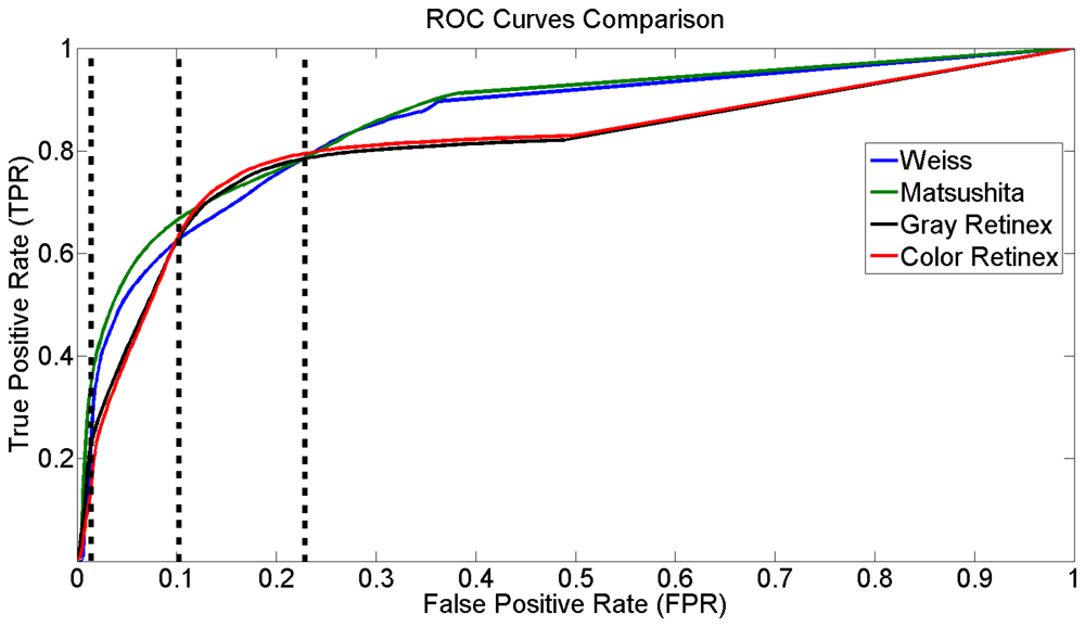
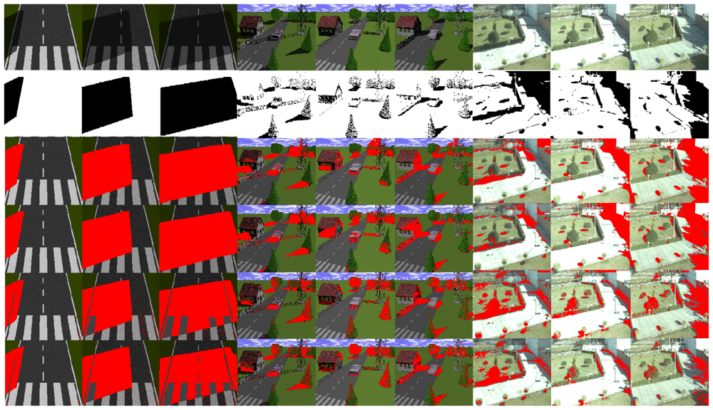
In this section, a quantitative assessment of the methods to detect shadows cast by urban infrastructure, based on the derived illumination image, is presented. To evaluate the performance of the methods systematically, we used the Receiver Operating Characteristic (ROC) analysis. For our evaluation, we used forty synthetic images (samples of these images are illustrated in fourth, fifth and sixth rows in Figure 5). The ground truth was computed automatically by subtracting the shadows from the shadowless image. First, the intrinsic image derivation methods were used to compute the reflectance and the illumination component of each frame. Then, a segmentation process based on the histogram analysis was applied. The curves in Figure 6 represent the false positive shadow detection rate on the horizontal axis and the shadow detection rate on the vertical one.

In addition, different performance results can be obtained for the methods in relation to the measuring parameter. For example, if we consider the value measured at the point in the ROC space that is located at the northwest point, the result would show that the best method to detect shadows based on the derived illumination image is color Retinex. Nonetheless, if we selected the area under the curve as a measurement parameter [44], the best method is that of Matsushita et al.

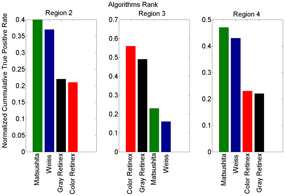
For a better analysis of Figure 6, we can consider the plots consisting of four regions. The first region R₁, according to the false positive rate, is between 0 and 0.01; the second region R₂ between 0.01 and 0.1; the third R₃ between 0.1 and 0.23, and the fourth one R₄ with larger values than the previous one (vertical lines Figure 6).

In R₁, all methods express similar behavior and thus it is not fair to rank them. In R₂, the method proposed by Matsushita et al has a performance that is superior to the others. In R₃, a mixture of information in the performance of the methods appears, while in R₄ a significant difference between the algorithms is apparent. In general, Figure 6 shows that there are two main tendencies in the efficiency of the methods, one for gray and color Retinex and the other for Weiss and Matsushita et al This is due to the fact that these two methods are very similar.

Figure 7 illustrates the ranking of the methods in the four regions of Figure 6. We used the normalized cumulative value of true positive rate (TPR) in each region to rank the methods. Based on these results, we considered the second region to extract and present the reflectance and illumination images in Figures 2 and 4. Moreover, all shadow detection results in Figure 5 were extracted from each respective data set with a 10% value for the false positive rate as the threshold parameter.

Figure 5 illustrates some shadow regions correctly detected. In the second row, the ground truth of shadows is illustrated. The ground truth of the shadows has been annotated manually to serve as a qualitative comparison between the methods to derive intrinsic images and the detection of shadows.

The Weiss [19] and Matsushita et al. [20] methods show better results than the strategies based on the Retinex algorithm [39,40]. The results of the Retinex algorithms applied to the synthetic sequence with white lines on the road surface are less effective than the other methods. The problem with the Retinex algorithm is that it is too constrained. It assumes that small values of the magnitude of the gradient are always due to changes in the illumination of the scene, but in general this idea is not always true.

In the second synthetic sequence, which consists of several static objects in an urban scenario, the methods can detect isolated shadows with good visual performance (see the pine tree and the tower in columns 4–6 in Figure 5). However, other objects such as the house and the trees that appear in the back part of the scene behind the tower, together with the sky line, have poor visual quality. These results are due to the remnant texture information present in the illumination component before the application of the shadow detection process. In the real images of Figure 5, variations in the intensity value of large shaded regions cause the algorithms to only be partially successful. As a result, some regions that have shadows are not well detected. For instance, the region at the right side of the image with the white brick wall (see columns 7–9) is not well detected by any of the discussed methods. The Weiss and Matsushita et al. methods fail because these regions are shaded all day, so this causes the shadow information to appear in the reflectance image. Similarly, the gray and color Retinex algorithms fail to detect large shadow areas, because the magnitude of the gradient in the shadow edges is similar to those caused by texture or color.

References

- Salvador, E.; Cavallaro, A.; Ebrahimi, T. Cast shadow segmentation using invariant color features. Comput. Vision Image Underst. 2004, 95, 238–259. [Google Scholar]
- Stander, J.; Mech, R.; Ostermann, J. Detection of moving cast shadows for object segmentation. Multimedia 1999, 1, 65–76. [Google Scholar]
- Xu, D.; Li, X.; Liu, Z.; Yuan, Y. Cast shadow detection in video segmentation. Pattern Recog. Lett. 2005, 26, 91–99. [Google Scholar]
- Foresti, G. Object recognition and tracking for remote video surveillance. IEEE Trans. Circuits Syst. Video Technol. 1999, 9, 1045–1062. [Google Scholar]
- Hsieh, J.; Hu, W.; Chang, C.; Chen, Y. Shadow elimination for effective moving object detection by gaussian shadow modeling. Image Vision Comput. 2003, 21, 505–516. [Google Scholar]
- Leone, A.; Distante, C. Shadow detection for moving objects based on texture analysis. Pattern Recog. 2007, 40, 1222–1233. [Google Scholar]
- Daum, M.; Dudek, G. On 3-D Surface Reconstruction Using Shape from Shadows. Proceedings of the IEEE Conference on Computer Vision and Pattern Recognition, Santa Barbara, CA, USA, 23–25 June 1998; pp. 461–468.
- Finlayson, G.; Hordley, S.; Lu, C.; Drew, M. On the removal of shadows from images. IEEE Trans. Pattern Anal. Mach. Intell. 2006, 28, 59–68. [Google Scholar]
- Poulin, A. Interactive Rendering of Trees with Shading and Shadows. Proceedings of the Rendering Techniques: Eurographics Workshop, London, UK, 25–27 June 2001; Springer Verlag Wien: Berlin/Heidelberg, Germany, 2001; pp. 183–196. [Google Scholar]
- Savarese, S.; Andreetto, M.; Rushmeier, H.; Bernardini, F.; Perona, P. 3D Reconstruction by shadow carving: Theory and practical evaluation. Int. J. Comput. Vis. 2007, 71, 305–336. [Google Scholar]
- Nagao, M.; Matsuyama, T.; Ikeda, Y. Region extraction and shape analysis in aerial photographs. Comput. Graph. Image Process. 1979, 10, 195–223. [Google Scholar]
- Barnard, K.; Finlayson, G. Shadow Identification Using Colour Ratios. Proceedings of the 8th Color Imaging Conference, Scottsdale, AZ, USA, 7–10 November 2000; 2, pp. 97–101.
- Prati, A.; Mikic, I.; Trivedi, M.; Cucchiara, R. Detecting moving shadows: Algorithms and evaluation. IEEE Trans. Pattern Anal. Machine Intell. 2003, 25, 918–923. [Google Scholar]
- Heikkila, M.; Pietikainen, M. A texture-based method for modeling the background and detecting moving objects. IEEE Trans. Pattern Anal. Machine Intell. 2006, 28, 657–662. [Google Scholar]
- Sanin, A.; Sanderson, C.; Lovell, B. Shadow detection: A survey and comparative evaluation of recent methods. Pattern Recog. 2012, 45, 1684–1695. [Google Scholar]
- Prati, A.; Cucchiara, R.; Mikic, I.; Trivedi, M. Analysis and Detection of Shadows in Video Streams: A Comparative Evaluation. Proceedings of the IEEE Conference on Computer Vision and Pattern Recognition, Kauai, HI, USA, 8–14 December 2001; 2, pp. 571–576.
- Isaza, C.; Salas, J.; Raducanu, B. Toward the Detection of Urban Infrastructure's Edge Shadows. In Advanced Concepts for Intelligent Vision Systems; Springer: Berlin/Heidelberg, Germany, 2010; pp. 30–37. [Google Scholar]
- Barrow, H.; Tenenbaum, J. Recovering Intrinsic Scene Characteristics from Images; Artificial Intelligence Center, SRI International: Menlo Park, CA, USA, 1978. [Google Scholar]
- Weiss, Y. Deriving Intrinsic Images from Image Sequences. Proceedings of the IEEE International Conference on Computer Vision, Vancouver, BC, Canada, 7–14 July, 2001; 2, pp. 68–75.
- Matsushita, Y.; Nishino, K.; Ikeuchi, K.; Sakauchi, M. Illumination normalization with time-dependent intrinsic images for video surveillance. IEEE Trans. Pattern Anal. Machine Intell. 2004, 26, 1336–1347. [Google Scholar]
- Blake, A. Boundary conditions for lightness computation in mondrian world. Comput. Vis., Graph., Image Process. 1985, 32, 314–327. [Google Scholar]
- Grosse, R.; Johnson, M.; Adelson, E.; Freeman, W. Ground Truth Dataset and Baseline Evaluations for Intrinsic Image Algorithms. Proceedings of the IEEE International Conference on Computer Vision, Kyoto, Japan, 27 September–4 October 2009; pp. 2335–2342.
- Kawasaki, H.; Furukawa, R. Shape Reconstruction from Cast Shadows Using Coplanarities and Metric Constraints. Proceedings of Asian Conference on Computer Vision, Tokyo, Japan, 18–22 November 2007; pp. 847–857.
- Kennedy, J. A Psychology of Picture Perception; Jossey-Bass: Oxford, England, 1974. [Google Scholar]
- Scanlan, J.; Chabries, D.; Christiansen, R. A Shadow Detection and Removal Algorithm for 2-D Images. Proceedings of the IEEE International Conference on Acoustics, Speech, and Signal Processing, Albuquerque, NM, USA, 3–6 April 1990; pp. 2057–2060.
- Jiang, C.; Ward, M. Shadow Identification. Proceedings of the IEEE Computer Society Conference on Computer Vision and Pattern Recognition, Champaign, IL, USA, 15–18 June 1992; pp. 606–612.
- Suzuki, A.; Shio, A.; Arai, H.; Ohtsuka, S. Dynamic Shadow Compensation of Aerial Images Based on Color and Spatial Analysis. Proceedings of the IEEE International Conference on Pattern Recognition, Barcelona, Spain, 5 September 2000; 1, pp. 317–320.
- Gevers, T.; Smeulders, W. Color based object recognition. Pattern Recog. 1999, 32, 453–464. [Google Scholar]
- Finlayson, G.; Hordley, S.; Drew, M. Removing Shadows from Images. Proceedings of European Conference on Computer Vision, Copenhagen, Denmark, 27 May 2002; pp. 129–132.
- Gevers, T.; Stokman, H. Classifying Color Transitions into Shadow-geometry, Illumination, Highlight or Material Edges. Proceedings of the IEEE International Conference on Image Processing, Vancouver, BC, Canada, 10–13 September 2000; 1, pp. 521–524.
- Levine, M.; Bhattacharyya, J. Removing shadows. Pattern Recog. Lett. 2005, 26, 251–265. [Google Scholar]
- Sonoda, Y.; Ogata, T. Separation of Moving Objects and Their Shadows, and Application to Tracking of Loci in the Monitoring Images. Proceedings of the IEEE International Conference on Signal Processing Proceedings, Santa Barbara, CA, USA, 12–16 October 1998; 2, pp. 1261–1264.
- Horprasert, T.; Harwood, D.; Davis, L. A Statistical Approach for Real-Time Robust Background Subtraction and Shadow Detection. Proceedings of the IEEE International Conference on Computer Vision, Kerkyra, Corfu, Greece, 20–25 September 1999; 99, pp. 256–261.
- Mikic, I.; Cosman, P.; Kogut, G.; Trivedi, M. Moving Shadow and Object Detection in Traffic Scenes. Proceedings of the IEEE International Conference on Pattern Recognition, Barcelona, Spain, 3–8 September 2000; 1, pp. 321–324.
- Nadimi, S.; Bhanu, B. Moving Shadow Detection Using a Physics-based Approach. Proceedings of the IEEE International Conference on Pattern Recognition, Quebec City, PQ, Canada, 1–15 August 2002; 2, pp. 701–704.
- Bevilacqua, A.; Roffilli, M. Robust Denoising and Moving Shadows Detection in Traffic Scenes. Proceedings of the IEEE Internatinoal Conference on Computer Vision and Pattern Recognition, Kauai, HI, USA, 8–14 December 2001; pp. 1–4.
- Cucchiara, R.; Grana, C.; Piccardi, M.; Prati, A. Detecting Objects, Shadows and Ghosts in Video Streams by Exploiting Color and Motion Information. Proceedings of the IEEE International Conference on Image Analysis and Processing, Palermo, Italy, 26–28 September 2001; pp. 360–365.
- The Persistence of Vision Raytracer Pty. Ltd. The Persistence of Vision Raytracer, Available online: http://www.povray.org (accessed on 31 January 2012).
- Land, E.; McCann, J. Lightness and retinex theory. J. Opt. Soc. Am. 1971, 61, 1–11. [Google Scholar]
- Finlayson, G.D.; Hordley, S.D.; Drew, M.S. Removing Shadows from Images Using Retinex. Proceedings of the Color Science and Engineering Systems, Technologies, and Applications. Color Imaging Conference, Scottsdale, AZ, USA, 12 November 2002; pp. 73–79.
- Reda, I.; Andreas, A. Solar position algorithm for solar radiation applications. Solar Energy 2004, 76, 577–589. [Google Scholar]
- Tappen, M.; Freeman, W.; Adelson, E. Recovering intrinsic images from a single image. Pattern Anal. Machine Intell. 2005, 27, 1459–1472. [Google Scholar]
- Huang, J.; Mumford, D. Statistics of Natural Images and Models. Proceedings of the IEEE Conference on Computer Vision and Pattern Recognition, Fort Collins, CO, USA, 23–25 June 1999; 1, pp. 541–547.
- Bradley, A. The use of the area under the ROC curve in the evaluation of machine learning algorithms. Pattern Recog. 1997, 30, 1145–1159. [Google Scholar]
© 2012 by the authors; licensee MDPI, Basel, Switzerland. This article is an open access article distributed under the terms and conditions of the Creative Commons Attribution license (http://creativecommons.org/licenses/by/3.0/).
Share and Cite
Isaza, C.; Salas, J.; Raducanu, B. Evaluation of Intrinsic Image Algorithms to Detect the Shadows Cast by Static Objects Outdoors. Sensors 2012, 12, 13333-13348. https://doi.org/10.3390/s121013333
Isaza C, Salas J, Raducanu B. Evaluation of Intrinsic Image Algorithms to Detect the Shadows Cast by Static Objects Outdoors. Sensors. 2012; 12(10):13333-13348. https://doi.org/10.3390/s121013333
Chicago/Turabian StyleIsaza, Cesar, Joaquín Salas, and Bogdan Raducanu. 2012. "Evaluation of Intrinsic Image Algorithms to Detect the Shadows Cast by Static Objects Outdoors" Sensors 12, no. 10: 13333-13348. https://doi.org/10.3390/s121013333