<?xml version="1.0" encoding="UTF-8"?>
<!DOCTYPE article PUBLIC "-//NLM//DTD Journal Publishing DTD v2.3 20070202//EN" "journalpublishing.dtd">
<article xmlns:mml="http://www.w3.org/1998/Math/MathML" xmlns:xlink="http://www.w3.org/1999/xlink" xml:lang="en" article-type="research-article">
<front>
<journal-meta>
<journal-id journal-id-type="nlm-ta">Sensors</journal-id>
<journal-title>Sensors</journal-title>
<issn pub-type="epub">1424-8220</issn>
<publisher>
<publisher-name>Molecular Diversity Preservation International (MDPI)</publisher-name></publisher></journal-meta>
<article-meta>
<article-id pub-id-type="doi">10.3390/s121012927</article-id>
<article-id pub-id-type="publisher-id">sensors-12-12927</article-id>
<article-categories>
<subj-group>
<subject>Article</subject></subj-group></article-categories>
<title-group>
<article-title>Front-Crawl Instantaneous Velocity Estimation Using a Wearable Inertial Measurement Unit</article-title></title-group>
<contrib-group>
<contrib contrib-type="author">
<name><surname>Dadashi</surname><given-names>Farzin</given-names></name><xref ref-type="aff" rid="af1-sensors-12-12927"><sup>1</sup></xref><xref ref-type="corresp" rid="c1-sensors-12-12927"><sup>*</sup></xref></contrib>
<contrib contrib-type="author">
<name><surname>Crettenand</surname><given-names>Florent</given-names></name><xref ref-type="aff" rid="af2-sensors-12-12927"><sup>2</sup></xref></contrib>
<contrib contrib-type="author">
<name><surname>Millet</surname><given-names>Grégoire P.</given-names></name><xref ref-type="aff" rid="af2-sensors-12-12927"><sup>2</sup></xref></contrib>
<contrib contrib-type="author">
<name><surname>Aminian</surname><given-names>Kamiar</given-names></name><xref ref-type="aff" rid="af1-sensors-12-12927"><sup>1</sup></xref></contrib></contrib-group>
<aff id="af1-sensors-12-12927">
<label>1</label> Laboratory of Movement Analysis and Measurement, École Polytechnique Fédérale de Lausanne (EPFL), 1015 Lausanne, Switzerland; E-Mail: <email>kamiar.aminian@epfl.ch</email></aff>
<aff id="af2-sensors-12-12927">
<label>2</label> Institute of Sport Sciences, University of Lausanne, 1015 Lausanne, Switzerland; E-Mails: <email>florent.crettenand@unil.ch</email> (F.C.); <email>gregoire.millet@unil.ch</email> (G.P.M.)</aff>
<author-notes>
<corresp id="c1-sensors-12-12927">
<label>*</label> Author to whom correspondence should be addressed; E-Mail: <email>farzin.dadashi@epfl.ch</email>; Tel.: +41-21-693-4773; Fax: +41-21-693-6915.</corresp></author-notes>
<pub-date pub-type="collection">
<year>2012</year></pub-date>
<pub-date pub-type="epub">
<day>25</day>
<month>09</month>
<year>2012</year></pub-date>
<volume>12</volume>
<issue>10</issue>
<fpage>12927</fpage>
<lpage>12939</lpage>
<history>
<date date-type="received">
<day>31</day>
<month>07</month>
<year>2012</year></date>
<date date-type="rev-recd">
<day>17</day>
<month>09</month>
<year>2012</year></date>
<date date-type="accepted">
<day>17</day>
<month>09</month>
<year>2012</year></date></history>
<permissions>
<copyright-statement>© 2012 by the authors; licensee MDPI, Basel, Switzerland.</copyright-statement>
<copyright-year>2012</copyright-year>
<license>
<p>This article is an open access article distributed under the terms and conditions of the Creative Commons Attribution license (http://creativecommons.org/licenses/by/3.0/).</p></license></permissions>
<abstract>
<p>Monitoring the performance is a crucial task for elite sports during both training and competition. Velocity is the key parameter of performance in swimming, but swimming performance evaluation remains immature due to the complexities of measurements in water. The purpose of this study is to use a single inertial measurement unit (IMU) to estimate front crawl velocity. Thirty swimmers, equipped with an IMU on the sacrum, each performed four different velocity trials of 25 m in ascending order. A tethered speedometer was used as the velocity measurement reference. Deployment of biomechanical constraints of front crawl locomotion and change detection framework on acceleration signal paved the way for a drift-free integration of forward acceleration using IMU to estimate the swimmers velocity. A difference of 0.6 ± 5.4 cm·s<sup>−1</sup> on mean cycle velocity and an RMS difference of 11.3 cm·s<sup>−1</sup> in instantaneous velocity estimation were observed between IMU and the reference. The most important contribution of the study is a new practical tool for objective evaluation of swimming performance. A single body-worn IMU provides timely feedback for coaches and sport scientists without any complicated setup or restraining the swimmer's natural technique.</p></abstract>
<kwd-group>
<kwd>accelerometer</kwd>
<kwd>gyroscope</kwd>
<kwd>biomechanical constraint</kwd>
<kwd>strap-down integration</kwd>
<kwd>swimming velocity</kwd></kwd-group></article-meta></front>
<body>
<sec sec-type="intro">
<label>1.</label>
<title>Introduction</title>
<p>The advent of new technologies has changed the perception of athletic achievement. In swimming, the narrow gap between record holders, points to the growing importance of devising new tools to assess self-improvement and optimize the training process. However, the biomechanical analysis of swimming remains inadequately explored due to complications of kinematics measurements in water.</p>
<p>To date, the most common practice for performance monitoring in swimming is using video-based systems. A video sequence is captured and post-processed through digitization [<xref ref-type="bibr" rid="b1-sensors-12-12927">1</xref>,<xref ref-type="bibr" rid="b2-sensors-12-12927">2</xref>]. The main downside of such systems is being excessively time consuming and problematic to fully automate. The application of this class of methods can be severely restricted by factors such as light refraction in water or bubbles generated around the swimmers' bodies [<xref ref-type="bibr" rid="b3-sensors-12-12927">3</xref>]. Recently a markerless 3D analysis method was proposed [<xref ref-type="bibr" rid="b4-sensors-12-12927">4</xref>] based on extraction of a swimmer's silhouette. This method reduced the video processing time, while still being sensitive to different lighting condition that leads to misidentification of features [<xref ref-type="bibr" rid="b5-sensors-12-12927">5</xref>].</p>
<p>The second category of techniques uses tethered monitoring. An early version of such a system was developed by Craig <italic>et al.</italic> [<xref ref-type="bibr" rid="b6-sensors-12-12927">6</xref>]. Velocity is directly measured by a cord attached to the swimmer. The cord is tethered to a poolside shaft-encoder [<xref ref-type="bibr" rid="b7-sensors-12-12927">7</xref>,<xref ref-type="bibr" rid="b8-sensors-12-12927">8</xref>]. Although this system is considered as reference to assess swimming velocity, the device disturbs the swimmers' technique and measures the velocity only in the forward direction. Moreover, the system requires a resisting force to tighten the cord during the decelerations of swimmer for an accurate measurement. Hence, this force is constantly applied to the swimmer.</p>
<p>During the past two decades inertial measurement units (IMUs) have been proven to be powerful tools in human movement analysis [<xref ref-type="bibr" rid="b9-sensors-12-12927">9</xref>]. First and foremost the portability of IMUs made them a viable system in daily life measurements, contrary to most other measurement systems which are restricted to laboratory conditions. Besides, the technological developments in microelectromechanical systems (MEMS) have made IMUs a low cost option compared to in-laboratory settings. The application of IMUs for sport analysis is a new trend in sport biomechanics [<xref ref-type="bibr" rid="b10-sensors-12-12927">10</xref>–<xref ref-type="bibr" rid="b12-sensors-12-12927">12</xref>]. A considerable number of studies have been conducted on the application of IMUs in the swimming context. Chronologically, Ohgi <italic>et al.</italic> [<xref ref-type="bibr" rid="b13-sensors-12-12927">13</xref>] were probably the first to use a wrist-worn IMU to detect front crawl and breast stroke swimming phases automatically. A sacrum mounted 3D accelerometer was used by Davey <italic>et al.</italic> [<xref ref-type="bibr" rid="b14-sensors-12-12927">14</xref>] to automatically extract simple metrics such as lap time and stroke rate. An IMU comprising a 3D accelerometer, 2D gyroscope and RF transceiver was used by Le Sage <italic>et al.</italic> [<xref ref-type="bibr" rid="b15-sensors-12-12927">15</xref>] to characterize swimming strokes in real time. However, none of aforementioned works involved kinematic measurements using IMUs. Recently, Stamm <italic>et al.</italic> [<xref ref-type="bibr" rid="b16-sensors-12-12927">16</xref>] published a method using a 3D accelerometer on the lower back to measure the front crawl velocity. However, a single 3D accelerometer generally is not capable of measuring the orientation of the body during dynamic movement. Consequently, the effect of lateral and vertical acceleration of swimmer's body cannot be removed from acceleration in the forward direction of swimming, therefore, calculating the integral of the acceleration signal in [<xref ref-type="bibr" rid="b16-sensors-12-12927">16</xref>] to evaluate the velocity can be misleading. Besides, it is well known that the accuracy of IMU-based systems in velocity measurement rapidly degrades over time due to inherent sensor noises [<xref ref-type="bibr" rid="b17-sensors-12-12927">17</xref>]. Hence special considerations are needed for a reliable assessment of velocity.</p>
<p>Considering the velocity as the most intuitive metric of swimmers' performance, this study aimed to propose a new method to measure swimming velocity in front crawl, using a single body-worn inertial sensor. We hypothesize that the swimmer's instantaneous velocity can be estimated accurately from IMU measurements when the average velocity of the swimmer over the trial is known. Drift-free integration of acceleration was certified in this study by assuming some simple locomotion constraints of the front crawl. Experimental protocols and statistical tools are introduced to assess the validity of the cycle and instantaneous velocity estimation method.</p></sec>
<sec>
<label>2.</label>
<title>Experimental Section</title>
<sec sec-type="subjects">
<label>2.1.</label>
<title>Participants and Protocol</title>
<p>Eleven elite and nineteen recreational swimmers took part in this study. Their attributes are shown in <xref ref-type="table" rid="t1-sensors-12-12927">Table 1</xref>. Each participant was informed of the procedures and risks associated with study participation and gave written informed consent prior to participation. This study was performed in accordance with the Declaration of Helsinki and was approved by the Ethics Committee of the Faculty of Biology and Medicine, University of Lausanne (protocol #87/10).</p>
<p>Each swimmer performed consecutive 25 m front-crawl trials in four different increasing velocity trials from 70% to 100% of their best personal 100 m timing recorded one month before the measurement. In case the performance time was different more than ±5% from the targeted time, the swimmer repeated the trial. They were asked to position in the water at the edge of the pool for starts.</p></sec>
<sec sec-type="methods">
<label>2.2.</label>
<title>Data Acquisition and Calibration</title>
<p>
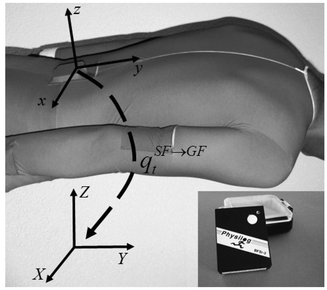
The swimmers were equipped with one waterproofed inertial sensor (Physilog<sup>®</sup>, BioAGM, La Tour-de-Peilz, Switzerland) including a 3D accelerometer (±11 g) and a 3D gyroscope (±900 °/s) and embedded data logger recording at 500 Hz. The sensor was worn on the sacrum inside the pocket of a custom designed swimming suit with a Velcro closing as shown in <xref ref-type="fig" rid="f1-sensors-12-12927">Figure 1</xref>. According to the feedback from swimmers, by wearing the sensor attachment in our study they did not feel the IMU imposed a noticeable drag during their training. The sensor was calibrated for offset, scale and non-orthogonality using in-field calibration procedure [<xref ref-type="bibr" rid="b18-sensors-12-12927">18</xref>].</p>
<p>As reference system, a tethered apparatus (SpeedRT<sup>®</sup>, ApLab, Rome, Italy) [<xref ref-type="bibr" rid="b8-sensors-12-12927">8</xref>] was attached to the waist of swimmers just beneath the lower end of the sensor with a belt. The system calculates the velocity by measuring the cord displacement through time at 100 Hz recording. The resistance applied to keep the cord tight is adjustable via a clutch on the pulley compartment of the apparatus. In our measurement, the resistance was set to 500 g [<xref ref-type="bibr" rid="b19-sensors-12-12927">19</xref>]. Since the tethered reference is installed on the starting block above the swimming level, the SpeedRT<sup>®</sup> cord is not parallel to the direction of swimming and imposes the parallax problem [<xref ref-type="bibr" rid="b15-sensors-12-12927">15</xref>]. By knowing the cord displacement at each time instant and the fact that the reference pulley was positioned 72 ± 1 cm above still pool water level, we calculated the instantaneous velocity measured by the reference in the swimming direction.</p></sec>
<sec>
<label>2.3.</label>
<title>Estimation of Swimming Orientation Using IMU</title>
<p>Instantaneous velocity is estimated by integrating the forward acceleration signal in the global frame (<italic>GF: X, Y, Z</italic>) (<xref ref-type="fig" rid="f1-sensors-12-12927">Figure 1</xref>). Among the axes of <italic>GF</italic> the <italic>Z</italic> is assumed to be vertically upward and <italic>Y</italic> in parallel with the longitudinal edge of the pool. The acceleration in <italic>GF</italic> can be calculated from the acceleration measured in sensor frame (<italic>SF: x, y, z</italic>) by considering the orientation of <italic>SF</italic> relative to <italic>GF</italic> at each time sample. The following paragraphs describe the required steps.</p>
<p>By starting the trials from a relatively motionless posture in water, the initial sacrum acceleration
<inline-formula>
<mml:math id="mm1" display="inline">
<mml:semantics id="sm1">
<mml:mrow>
<mml:msubsup>
<mml:mi>a</mml:mi>
<mml:mn>0</mml:mn>
<mml:mtext mathvariant="italic">SF</mml:mtext></mml:msubsup>
<mml:mo>=</mml:mo>
<mml:msup>
<mml:mrow>
<mml:mrow>
<mml:mo>[</mml:mo>
<mml:mrow>
<mml:msubsup>
<mml:mi>a</mml:mi>
<mml:mn>0</mml:mn>
<mml:mi>x</mml:mi></mml:msubsup>
<mml:mo>,</mml:mo>
<mml:msubsup>
<mml:mi>a</mml:mi>
<mml:mn>0</mml:mn>
<mml:mi>y</mml:mi></mml:msubsup>
<mml:mo>,</mml:mo>
<mml:msubsup>
<mml:mi>a</mml:mi>
<mml:mn>0</mml:mn>
<mml:mi>z</mml:mi></mml:msubsup></mml:mrow>
<mml:mo>]</mml:mo></mml:mrow></mml:mrow>
<mml:mi>T</mml:mi></mml:msup></mml:mrow></mml:semantics></mml:math></inline-formula> has a magnitude equal to the gravity. Using quaternion based algebra to represent the orientation, the initial quaternion which aligns the <italic>z</italic> axis to <italic>Z</italic>, is given by:
<disp-formula id="FD1">
<label>(1)</label>
<mml:math id="mm2" display="block">
<mml:semantics id="sm2">
<mml:mrow>
<mml:msubsup>
<mml:mi>q</mml:mi>
<mml:mi>t</mml:mi>
<mml:mrow>
<mml:mtext mathvariant="italic">SF</mml:mtext>
<mml:mo>→</mml:mo>
<mml:mtext mathvariant="italic">GF</mml:mtext></mml:mrow></mml:msubsup>
<mml:mo>=</mml:mo>
<mml:mrow>
<mml:mo stretchy="true">[</mml:mo>
<mml:mrow>
<mml:mo>cos</mml:mo>
<mml:mfrac>
<mml:mrow>
<mml:msub>
<mml:mi>θ</mml:mi>
<mml:mn>0</mml:mn></mml:msub></mml:mrow>
<mml:mn>2</mml:mn></mml:mfrac>
<mml:mo>,</mml:mo>
<mml:mfrac>
<mml:mrow>
<mml:msub>
<mml:mi>u</mml:mi>
<mml:mn>0</mml:mn></mml:msub></mml:mrow>
<mml:mrow>
<mml:mrow>
<mml:mo>‖</mml:mo>
<mml:mrow>
<mml:msub>
<mml:mi>u</mml:mi>
<mml:mn>0</mml:mn></mml:msub></mml:mrow>
<mml:mo>‖</mml:mo></mml:mrow></mml:mrow></mml:mfrac>
<mml:mo>sin</mml:mo>
<mml:mfrac>
<mml:mrow>
<mml:msub>
<mml:mi>θ</mml:mi>
<mml:mn>0</mml:mn></mml:msub></mml:mrow>
<mml:mn>2</mml:mn></mml:mfrac></mml:mrow>
<mml:mo stretchy="true">]</mml:mo></mml:mrow></mml:mrow></mml:semantics></mml:math></disp-formula>where, ‖.‖ represents Euclidian norm, <italic>θ</italic><sub>0</sub> is the initial inclination and <italic>u<sub>0</sub></italic> represents the horizontal axis around which the rotation is done. Supposing that azimuth angle at start of trial is null, <italic>θ</italic><sub>0</sub> and <italic>u<sub>0</sub></italic> can be calculated as in <xref rid="FD2" ref-type="disp-formula">Equation (2)</xref> and <xref rid="FD3" ref-type="disp-formula">Equation (3)</xref>, respectively:
<disp-formula id="FD2">
<label>(2)</label>
<mml:math id="mm3" display="block">
<mml:semantics id="sm3">
<mml:mrow>
<mml:msub>
<mml:mi>θ</mml:mi>
<mml:mn>0</mml:mn></mml:msub>
<mml:mo>=</mml:mo>
<mml:msup>
<mml:mrow>
<mml:mo>cos</mml:mo></mml:mrow>
<mml:mrow>
<mml:mo>−</mml:mo>
<mml:mn>1</mml:mn></mml:mrow></mml:msup>
<mml:mo stretchy="false">(</mml:mo>
<mml:mo>−</mml:mo>
<mml:msubsup>
<mml:mi>a</mml:mi>
<mml:mn>0</mml:mn>
<mml:mtext mathvariant="italic">SF</mml:mtext></mml:msubsup>
<mml:mo>.</mml:mo>
<mml:msup>
<mml:mi>Z</mml:mi>
<mml:mrow>
<mml:mtext mathvariant="italic">GF</mml:mtext></mml:mrow></mml:msup>
<mml:mo stretchy="false">)</mml:mo></mml:mrow></mml:semantics></mml:math></disp-formula>
<disp-formula id="FD3">
<label>(3)</label>
<mml:math id="mm4" display="block">
<mml:semantics id="sm4">
<mml:mrow>
<mml:msub>
<mml:mi>u</mml:mi>
<mml:mn>0</mml:mn></mml:msub>
<mml:mo>=</mml:mo>
<mml:mo>−</mml:mo>
<mml:msubsup>
<mml:mi>a</mml:mi>
<mml:mn>0</mml:mn>
<mml:mtext mathvariant="italic">SF</mml:mtext></mml:msubsup>
<mml:mo>×</mml:mo>
<mml:msup>
<mml:mi>Z</mml:mi>
<mml:mtext mathvariant="italic">GF</mml:mtext></mml:msup>
<mml:mo>=</mml:mo>
<mml:mrow>
<mml:mo>[</mml:mo>
<mml:mrow>
<mml:mo>−</mml:mo>
<mml:msubsup>
<mml:mi>a</mml:mi>
<mml:mn>0</mml:mn>
<mml:mi>y</mml:mi></mml:msubsup>
<mml:mo>,</mml:mo>
<mml:msubsup>
<mml:mi>a</mml:mi>
<mml:mn>0</mml:mn>
<mml:mi>x</mml:mi></mml:msubsup>
<mml:mo>,</mml:mo>
<mml:mn>0</mml:mn></mml:mrow>
<mml:mo>]</mml:mo></mml:mrow></mml:mrow></mml:semantics></mml:math></disp-formula>where × represents the normal cross product.</p>
<p>At each time step <italic>t</italic>, the orientation of <italic>SF</italic> relative to <italic>GF</italic>,
<inline-formula>
<mml:math id="mm5" display="inline">
<mml:semantics id="sm5">
<mml:mrow>
<mml:msubsup>
<mml:mi>q</mml:mi>
<mml:mi>t</mml:mi>
<mml:mrow>
<mml:mtext mathvariant="italic">SF</mml:mtext>
<mml:mo>→</mml:mo>
<mml:mtext mathvariant="italic">GF</mml:mtext></mml:mrow></mml:msubsup></mml:mrow></mml:semantics></mml:math></inline-formula> is updated using the previous orientation by integrating the angular velocity 
<inline-formula>
<mml:math id="mm6" display="inline">
<mml:semantics id="sm6">
<mml:mrow>
<mml:msubsup>
<mml:mi>ω</mml:mi>
<mml:mi>t</mml:mi>
<mml:mrow>
<mml:mtext mathvariant="italic">SF</mml:mtext></mml:mrow></mml:msubsup>
<mml:mo>=</mml:mo>
<mml:msup>
<mml:mrow>
<mml:mrow>
<mml:mo>[</mml:mo>
<mml:mrow>
<mml:msubsup>
<mml:mi>ω</mml:mi>
<mml:mi>t</mml:mi>
<mml:mi>x</mml:mi></mml:msubsup>
<mml:mo>,</mml:mo>
<mml:msubsup>
<mml:mi>ω</mml:mi>
<mml:mi>t</mml:mi>
<mml:mi>y</mml:mi></mml:msubsup>
<mml:mo>,</mml:mo>
<mml:msubsup>
<mml:mi>ω</mml:mi>
<mml:mi>t</mml:mi>
<mml:mi>z</mml:mi></mml:msubsup></mml:mrow>
<mml:mo>]</mml:mo></mml:mrow></mml:mrow>
<mml:mi>T</mml:mi></mml:msup></mml:mrow></mml:semantics></mml:math></inline-formula> [<xref ref-type="bibr" rid="b20-sensors-12-12927">20</xref>]:
<disp-formula id="FD4">
<label>(4)</label>
<mml:math id="mm7" display="block">
<mml:semantics id="sm7">
<mml:mrow>
<mml:msubsup>
<mml:mi>q</mml:mi>
<mml:mi>t</mml:mi>
<mml:mrow>
<mml:mtext mathvariant="italic">SF</mml:mtext>
<mml:mo>→</mml:mo>
<mml:mtext mathvariant="italic">GF</mml:mtext></mml:mrow></mml:msubsup>
<mml:mo>=</mml:mo>
<mml:mrow>
<mml:mo stretchy="true">[</mml:mo>
<mml:mrow>
<mml:mo>cos</mml:mo>
<mml:mrow>
<mml:mo stretchy="true">(</mml:mo>
<mml:mrow>
<mml:mfrac>
<mml:mrow>
<mml:mrow>
<mml:mo>‖</mml:mo>
<mml:mrow>
<mml:msubsup>
<mml:mi>ω</mml:mi>
<mml:mi>t</mml:mi>
<mml:mrow>
<mml:mtext mathvariant="italic">SF</mml:mtext></mml:mrow></mml:msubsup></mml:mrow>
<mml:mo>‖</mml:mo></mml:mrow></mml:mrow>
<mml:mrow>
<mml:mn>2</mml:mn>
<mml:mi>f</mml:mi></mml:mrow></mml:mfrac></mml:mrow>
<mml:mo stretchy="true">)</mml:mo></mml:mrow>
<mml:mo>,</mml:mo>
<mml:mfrac>
<mml:mrow>
<mml:msubsup>
<mml:mi>ω</mml:mi>
<mml:mi>t</mml:mi>
<mml:mrow>
<mml:mtext mathvariant="italic">SF</mml:mtext></mml:mrow></mml:msubsup></mml:mrow>
<mml:mrow>
<mml:mrow>
<mml:mo>‖</mml:mo>
<mml:mrow>
<mml:msubsup>
<mml:mi>ω</mml:mi>
<mml:mi>t</mml:mi>
<mml:mrow>
<mml:mtext mathvariant="italic">SF</mml:mtext></mml:mrow></mml:msubsup></mml:mrow>
<mml:mo>‖</mml:mo></mml:mrow></mml:mrow></mml:mfrac>
<mml:mo>sin</mml:mo>
<mml:mrow>
<mml:mo stretchy="true">(</mml:mo>
<mml:mrow>
<mml:mfrac>
<mml:mrow>
<mml:mrow>
<mml:mo>‖</mml:mo>
<mml:mrow>
<mml:msubsup>
<mml:mi>ω</mml:mi>
<mml:mi>t</mml:mi>
<mml:mrow>
<mml:mtext mathvariant="italic">SF</mml:mtext></mml:mrow></mml:msubsup></mml:mrow>
<mml:mo>‖</mml:mo></mml:mrow></mml:mrow>
<mml:mrow>
<mml:mn>2</mml:mn>
<mml:mi>f</mml:mi></mml:mrow></mml:mfrac></mml:mrow>
<mml:mo stretchy="true">)</mml:mo></mml:mrow></mml:mrow>
<mml:mo stretchy="true">]</mml:mo></mml:mrow>
<mml:mo>⊗</mml:mo>
<mml:msubsup>
<mml:mi>q</mml:mi>
<mml:mrow>
<mml:mi>t</mml:mi>
<mml:mo>−</mml:mo>
<mml:mn>1</mml:mn></mml:mrow>
<mml:mrow>
<mml:mtext mathvariant="italic">SF</mml:mtext>
<mml:mo>→</mml:mo>
<mml:mtext mathvariant="italic">GF</mml:mtext></mml:mrow></mml:msubsup></mml:mrow></mml:semantics></mml:math></disp-formula>where <italic>f</italic> is sampling frequency and ⊗ indicates quaternion multiplication.</p>
<p>The time integration in <xref rid="FD4" ref-type="disp-formula">Equation (4)</xref> suffers from an accumulative drift [<xref ref-type="bibr" rid="b17-sensors-12-12927">17</xref>] due to gyroscopic noise. In order to reduce the effect of this drift we applied a dynamic biomechanical constraint, namely considering the swimmer sacrum rolls in average about forward direction <italic>Y</italic>. Therefore, for the data samples from cycle <italic>k</italic> to <italic>k</italic> + <italic>1</italic> (denoted by <italic>C<sub>k</sub></italic> and <italic>C<sub>k</sub></italic><sub>+1</sub> respectively), the principal component of angular velocity in <italic>GF</italic> (represented by 
<inline-formula>
<mml:math id="mm8" display="inline">
<mml:semantics id="sm8">
<mml:mrow>
<mml:mi>P</mml:mi>
<mml:msubsup>
<mml:mi>ω</mml:mi>
<mml:mrow>
<mml:msub>
<mml:mi>C</mml:mi>
<mml:mi>k</mml:mi></mml:msub></mml:mrow>
<mml:mrow>
<mml:mtext mathvariant="italic">GF</mml:mtext></mml:mrow></mml:msubsup></mml:mrow></mml:semantics></mml:math></inline-formula>) should be aligned to <italic>Y</italic>. This can be mathematically written as:
<disp-formula id="FD5">
<label>(5)</label>
<mml:math id="mm9" display="block">
<mml:semantics id="sm9">
<mml:mrow>
<mml:mtable>
<mml:mtr>
<mml:mtd>
<mml:mrow>
<mml:mi>P</mml:mi>
<mml:msubsup>
<mml:mi>ω</mml:mi>
<mml:mrow>
<mml:msub>
<mml:mi>C</mml:mi>
<mml:mi>k</mml:mi></mml:msub></mml:mrow>
<mml:mtext mathvariant="italic">GF</mml:mtext></mml:msubsup>
<mml:mo>=</mml:mo>
<mml:mtext mathvariant="italic">principle component</mml:mtext>
<mml:mo>(</mml:mo>
<mml:mrow>
<mml:mrow>
<mml:mo>(</mml:mo>
<mml:mrow>
<mml:msubsup>
<mml:mi>q</mml:mi>
<mml:mi>t</mml:mi>
<mml:mrow>
<mml:mtext mathvariant="italic">SF</mml:mtext>
<mml:mo>→</mml:mo>
<mml:mtext mathvariant="italic">GF</mml:mtext></mml:mrow></mml:msubsup></mml:mrow>
<mml:mo>)</mml:mo></mml:mrow>
<mml:mo>⊗</mml:mo>
<mml:msubsup>
<mml:mi>ω</mml:mi>
<mml:mi>t</mml:mi>
<mml:mtext mathvariant="italic">SF</mml:mtext></mml:msubsup>
<mml:mo>⊗</mml:mo>
<mml:msup>
<mml:mrow>
<mml:mrow>
<mml:mo>(</mml:mo>
<mml:mrow>
<mml:msubsup>
<mml:mi>q</mml:mi>
<mml:mi>t</mml:mi>
<mml:mrow>
<mml:mtext mathvariant="italic">SF</mml:mtext>
<mml:mo>→</mml:mo>
<mml:mtext mathvariant="italic">GF</mml:mtext></mml:mrow></mml:msubsup></mml:mrow>
<mml:mo>)</mml:mo></mml:mrow></mml:mrow>
<mml:mrow>
<mml:mo>−</mml:mo>
<mml:mn>1</mml:mn></mml:mrow></mml:msup></mml:mrow>
<mml:mo>)</mml:mo>
<mml:mo>≅</mml:mo>
<mml:mrow>
<mml:mo>[</mml:mo>
<mml:mrow>
<mml:mn>0</mml:mn>
<mml:mo>,</mml:mo>
<mml:mn>1</mml:mn>
<mml:mo>,</mml:mo>
<mml:mn>0</mml:mn></mml:mrow>
<mml:mo>]</mml:mo></mml:mrow></mml:mrow></mml:mtd>
<mml:mtd>
<mml:mrow>
<mml:mo>∀</mml:mo>
<mml:mi>t</mml:mi>
<mml:mo>:</mml:mo>
<mml:msub>
<mml:mi>C</mml:mi>
<mml:mi>k</mml:mi></mml:msub>
<mml:mo>≤</mml:mo>
<mml:mi>t</mml:mi>
<mml:mo>&lt;</mml:mo>
<mml:msub>
<mml:mi>C</mml:mi>
<mml:mrow>
<mml:mi>k</mml:mi>
<mml:mo>+</mml:mo>
<mml:mn>1</mml:mn></mml:mrow></mml:msub></mml:mrow></mml:mtd></mml:mtr></mml:mtable></mml:mrow></mml:semantics></mml:math></disp-formula></p>
<p>Any deviation from the conditions of <xref rid="FD5" ref-type="disp-formula">Equation (5)</xref> was assumed to be the effect of the orientation drift. <xref ref-type="fig" rid="f2-sensors-12-12927">Figure 2</xref> shows the deviation of one cycle from this condition. The amplitude of the drifted angle is given by <xref rid="FD6" ref-type="disp-formula">Equation (6)</xref>:
<disp-formula id="FD6">
<label>(6)</label>
<mml:math id="mm10" display="block">
<mml:semantics id="sm10">
<mml:mrow>
<mml:mi mathvariant="normal">Δ</mml:mi>
<mml:msub>
<mml:mi>θ</mml:mi>
<mml:mrow>
<mml:msub>
<mml:mi>C</mml:mi>
<mml:mi>k</mml:mi></mml:msub></mml:mrow></mml:msub>
<mml:mo>=</mml:mo>
<mml:msup>
<mml:mrow>
<mml:mo>cos</mml:mo></mml:mrow>
<mml:mrow>
<mml:mo>−</mml:mo>
<mml:mn>1</mml:mn></mml:mrow></mml:msup>
<mml:mrow>
<mml:mo stretchy="true">(</mml:mo>
<mml:mrow>
<mml:mfrac>
<mml:mrow>
<mml:mrow>
<mml:mo>[</mml:mo>
<mml:mrow>
<mml:mn>0</mml:mn>
<mml:mo>,</mml:mo>
<mml:mn>1</mml:mn>
<mml:mo>,</mml:mo>
<mml:mn>0</mml:mn></mml:mrow>
<mml:mo>]</mml:mo></mml:mrow>
<mml:mo>.</mml:mo>
<mml:mi>P</mml:mi>
<mml:msubsup>
<mml:mi>ω</mml:mi>
<mml:mrow>
<mml:msub>
<mml:mi>C</mml:mi>
<mml:mi>k</mml:mi></mml:msub></mml:mrow>
<mml:mtext mathvariant="italic">GF</mml:mtext></mml:msubsup></mml:mrow>
<mml:mrow>
<mml:mrow>
<mml:mo>‖</mml:mo>
<mml:mrow>
<mml:mi>P</mml:mi>
<mml:msubsup>
<mml:mi>ω</mml:mi>
<mml:mrow>
<mml:msub>
<mml:mi>C</mml:mi>
<mml:mi>k</mml:mi></mml:msub></mml:mrow>
<mml:mtext mathvariant="italic">GF</mml:mtext></mml:msubsup></mml:mrow>
<mml:mo>‖</mml:mo></mml:mrow></mml:mrow></mml:mfrac></mml:mrow>
<mml:mo stretchy="true">)</mml:mo></mml:mrow></mml:mrow></mml:semantics></mml:math></disp-formula></p>
<p>Accordingly the rotation axis is presented as in <xref rid="FD7" ref-type="disp-formula">Equation (7)</xref>:
<disp-formula id="FD7">
<label>(7)</label>
<mml:math id="mm11" display="block">
<mml:semantics id="sm11">
<mml:mrow>
<mml:msub>
<mml:mi>u</mml:mi>
<mml:mrow>
<mml:msub>
<mml:mi>C</mml:mi>
<mml:mi>k</mml:mi></mml:msub></mml:mrow></mml:msub>
<mml:mo>=</mml:mo>
<mml:mfrac>
<mml:mrow>
<mml:mrow>
<mml:mo>[</mml:mo>
<mml:mrow>
<mml:mn>0</mml:mn>
<mml:mo>,</mml:mo>
<mml:mn>1</mml:mn>
<mml:mo>,</mml:mo>
<mml:mn>0</mml:mn></mml:mrow>
<mml:mo>]</mml:mo></mml:mrow>
<mml:mo>×</mml:mo>
<mml:mi>P</mml:mi>
<mml:msubsup>
<mml:mi>ω</mml:mi>
<mml:mrow>
<mml:msub>
<mml:mi>C</mml:mi>
<mml:mi>k</mml:mi></mml:msub></mml:mrow>
<mml:mrow>
<mml:mtext mathvariant="italic">GF</mml:mtext></mml:mrow></mml:msubsup></mml:mrow>
<mml:mrow>
<mml:mrow>
<mml:mo>‖</mml:mo>
<mml:mrow>
<mml:mi>P</mml:mi>
<mml:msubsup>
<mml:mi>ω</mml:mi>
<mml:mrow>
<mml:msub>
<mml:mi>C</mml:mi>
<mml:mi>k</mml:mi></mml:msub></mml:mrow>
<mml:mrow>
<mml:mtext mathvariant="italic">GF</mml:mtext></mml:mrow></mml:msubsup></mml:mrow>
<mml:mo>‖</mml:mo></mml:mrow></mml:mrow></mml:mfrac></mml:mrow></mml:semantics></mml:math></disp-formula></p>
<p>So if we suppose that the drift is linearly increased through one cycle with <italic>n</italic> data points, for the <italic>t<sup>th</sup></italic> sample we can compute the corrective quaternion as in <xref rid="FD8" ref-type="disp-formula">Equation (8)</xref>:
<disp-formula id="FD8">
<label>(8)</label>
<mml:math id="mm12" display="block">
<mml:semantics id="sm12">
<mml:mrow>
<mml:mtable>
<mml:mtr>
<mml:mtd>
<mml:mrow>
<mml:mi>δ</mml:mi>
<mml:msub>
<mml:mi>q</mml:mi>
<mml:mi>t</mml:mi></mml:msub>
<mml:mo>=</mml:mo>
<mml:mrow>
<mml:mo stretchy="true">[</mml:mo>
<mml:mrow>
<mml:mo>cos</mml:mo>
<mml:mrow>
<mml:mo stretchy="true">(</mml:mo>
<mml:mrow>
<mml:mfrac>
<mml:mrow>
<mml:mi mathvariant="normal">Δ</mml:mi>
<mml:msub>
<mml:mi>θ</mml:mi>
<mml:mrow>
<mml:msub>
<mml:mi>C</mml:mi>
<mml:mi>k</mml:mi></mml:msub></mml:mrow></mml:msub></mml:mrow>
<mml:mrow>
<mml:mn>2</mml:mn>
<mml:mo stretchy="false">(</mml:mo>
<mml:mi>n</mml:mi>
<mml:mo>−</mml:mo>
<mml:mn>1</mml:mn>
<mml:mo stretchy="false">)</mml:mo></mml:mrow></mml:mfrac>
<mml:mo stretchy="false">(</mml:mo>
<mml:mi>t</mml:mi>
<mml:mo>−</mml:mo>
<mml:mn>1</mml:mn>
<mml:mo stretchy="false">)</mml:mo></mml:mrow>
<mml:mo stretchy="true">)</mml:mo></mml:mrow>
<mml:mo>,</mml:mo>
<mml:mfrac>
<mml:mrow>
<mml:msub>
<mml:mi>u</mml:mi>
<mml:mrow>
<mml:msub>
<mml:mi>C</mml:mi>
<mml:mi>k</mml:mi></mml:msub></mml:mrow></mml:msub></mml:mrow>
<mml:mrow>
<mml:mrow>
<mml:mo>‖</mml:mo>
<mml:mrow>
<mml:msub>
<mml:mi>u</mml:mi>
<mml:mrow>
<mml:msub>
<mml:mi>C</mml:mi>
<mml:mi>k</mml:mi></mml:msub></mml:mrow></mml:msub></mml:mrow>
<mml:mo>‖</mml:mo></mml:mrow></mml:mrow></mml:mfrac>
<mml:mo>sin</mml:mo>
<mml:mrow>
<mml:mo stretchy="true">(</mml:mo>
<mml:mrow>
<mml:mfrac>
<mml:mrow>
<mml:mi mathvariant="normal">Δ</mml:mi>
<mml:msub>
<mml:mi>θ</mml:mi>
<mml:mrow>
<mml:msub>
<mml:mi>C</mml:mi>
<mml:mi>k</mml:mi></mml:msub></mml:mrow></mml:msub></mml:mrow>
<mml:mrow>
<mml:mn>2</mml:mn>
<mml:mo stretchy="false">(</mml:mo>
<mml:mi>n</mml:mi>
<mml:mo>−</mml:mo>
<mml:mn>1</mml:mn>
<mml:mo stretchy="false">)</mml:mo></mml:mrow></mml:mfrac>
<mml:mo stretchy="false">(</mml:mo>
<mml:mi>t</mml:mi>
<mml:mo>−</mml:mo>
<mml:mn>1</mml:mn>
<mml:mo stretchy="false">)</mml:mo></mml:mrow>
<mml:mo stretchy="true">)</mml:mo></mml:mrow></mml:mrow>
<mml:mo stretchy="true">]</mml:mo></mml:mrow></mml:mrow></mml:mtd>
<mml:mtd>
<mml:mrow>
<mml:mo>∀</mml:mo>
<mml:mi>t</mml:mi>
<mml:mo>:</mml:mo>
<mml:msub>
<mml:mi>C</mml:mi>
<mml:mi>k</mml:mi></mml:msub>
<mml:mo>≤</mml:mo>
<mml:mi>t</mml:mi>
<mml:mo>&lt;</mml:mo>
<mml:msub>
<mml:mi>C</mml:mi>
<mml:mrow>
<mml:mi>k</mml:mi>
<mml:mo>+</mml:mo>
<mml:mn>1</mml:mn></mml:mrow></mml:msub></mml:mrow></mml:mtd></mml:mtr></mml:mtable></mml:mrow></mml:semantics></mml:math></disp-formula></p>
<p>Therefore, the corrected orientation of <italic>SF</italic> relative to <italic>GF</italic>, 
<inline-formula>
<mml:math id="mm13" display="inline">
<mml:semantics id="sm13">
<mml:mrow>
<mml:msubsup>
<mml:mi>q</mml:mi>
<mml:mrow>
<mml:mi>t</mml:mi>
<mml:mo>,</mml:mo>
<mml:msub>
<mml:mi>C</mml:mi>
<mml:mi>k</mml:mi></mml:msub></mml:mrow>
<mml:mrow>
<mml:mtext mathvariant="italic">SF</mml:mtext>
<mml:mo>→</mml:mo>
<mml:mtext mathvariant="italic">GF</mml:mtext></mml:mrow></mml:msubsup></mml:mrow></mml:semantics></mml:math></inline-formula> can be calculated from <xref rid="FD9" ref-type="disp-formula">Equation (9)</xref>:
<disp-formula id="FD9">
<label>(9)</label>
<mml:math id="mm14" display="block">
<mml:semantics id="sm14">
<mml:mrow>
<mml:msubsup>
<mml:mi>q</mml:mi>
<mml:mrow>
<mml:mi>t</mml:mi>
<mml:mo>,</mml:mo>
<mml:msub>
<mml:mi>C</mml:mi>
<mml:mi>k</mml:mi></mml:msub></mml:mrow>
<mml:mrow>
<mml:mtext mathvariant="italic">SF</mml:mtext>
<mml:mo>→</mml:mo>
<mml:mtext mathvariant="italic">GF</mml:mtext></mml:mrow></mml:msubsup>
<mml:mo>=</mml:mo>
<mml:mrow>
<mml:mo>(</mml:mo>
<mml:mrow>
<mml:msubsup>
<mml:mi>q</mml:mi>
<mml:mi>t</mml:mi>
<mml:mrow>
<mml:mtext mathvariant="italic">SF</mml:mtext>
<mml:mo>→</mml:mo>
<mml:mtext mathvariant="italic">GF</mml:mtext></mml:mrow></mml:msubsup></mml:mrow>
<mml:mo>)</mml:mo></mml:mrow>
<mml:mo>⊗</mml:mo>
<mml:mi>δ</mml:mi>
<mml:msub>
<mml:mi>q</mml:mi>
<mml:mi>t</mml:mi></mml:msub></mml:mrow></mml:semantics></mml:math></disp-formula></p>
<p>The instantaneous forward acceleration in global frame can be calculated according to <xref rid="FD10" ref-type="disp-formula">Equation (10)</xref>, where g⃗ shows the gravity vector:
<disp-formula id="FD10">
<label>(10)</label>
<mml:math id="mm15" display="block">
<mml:semantics id="sm15">
<mml:mrow>
<mml:msubsup>
<mml:mi>a</mml:mi>
<mml:mi>t</mml:mi>
<mml:mi>Y</mml:mi></mml:msubsup>
<mml:mo>=</mml:mo>
<mml:mrow>
<mml:mo>(</mml:mo>
<mml:mrow>
<mml:mrow>
<mml:mo>(</mml:mo>
<mml:mrow>
<mml:msubsup>
<mml:mi>q</mml:mi>
<mml:mrow>
<mml:mi>t</mml:mi>
<mml:mo>,</mml:mo>
<mml:msub>
<mml:mi>C</mml:mi>
<mml:mi>k</mml:mi></mml:msub></mml:mrow>
<mml:mrow>
<mml:mtext mathvariant="italic">SF</mml:mtext>
<mml:mo>→</mml:mo>
<mml:mtext mathvariant="italic">GF</mml:mtext></mml:mrow></mml:msubsup></mml:mrow>
<mml:mo>)</mml:mo></mml:mrow>
<mml:mo>⊗</mml:mo>
<mml:msubsup>
<mml:mi>a</mml:mi>
<mml:mi>t</mml:mi>
<mml:mrow>
<mml:mtext mathvariant="italic">SF</mml:mtext></mml:mrow></mml:msubsup>
<mml:mo>⊗</mml:mo>
<mml:msup>
<mml:mrow>
<mml:mrow>
<mml:mo>(</mml:mo>
<mml:mrow>
<mml:msubsup>
<mml:mi>q</mml:mi>
<mml:mrow>
<mml:mi>t</mml:mi>
<mml:mo>,</mml:mo>
<mml:msub>
<mml:mi>C</mml:mi>
<mml:mi>k</mml:mi></mml:msub></mml:mrow>
<mml:mrow>
<mml:mtext mathvariant="italic">SF</mml:mtext>
<mml:mo>→</mml:mo>
<mml:mtext mathvariant="italic">GF</mml:mtext></mml:mrow></mml:msubsup></mml:mrow>
<mml:mo>)</mml:mo></mml:mrow></mml:mrow>
<mml:mrow>
<mml:mo>−</mml:mo>
<mml:mn>1</mml:mn></mml:mrow></mml:msup>
<mml:mo>−</mml:mo>
<mml:mover accent="true">
<mml:mi>g</mml:mi>
<mml:mo>→</mml:mo></mml:mover></mml:mrow>
<mml:mo>)</mml:mo></mml:mrow>
<mml:mo>.</mml:mo>
<mml:mrow>
<mml:mo>(</mml:mo>
<mml:mrow>
<mml:mtable>
<mml:mtr>
<mml:mtd>
<mml:mn>0</mml:mn></mml:mtd></mml:mtr>
<mml:mtr>
<mml:mtd>
<mml:mn>1</mml:mn></mml:mtd></mml:mtr>
<mml:mtr>
<mml:mtd>
<mml:mn>0</mml:mn></mml:mtd></mml:mtr></mml:mtable></mml:mrow>
<mml:mo>)</mml:mo></mml:mrow></mml:mrow></mml:semantics></mml:math></disp-formula></p></sec>
<sec>
<label>2.4.</label>
<title>Instantaneous and Cycle Velocity Estimation</title>
<p>The instantaneous velocity <italic>V<sub>t</sub></italic> can be obtained by trapezoidal integration of
<inline-formula>
<mml:math id="mm16" display="inline">
<mml:semantics id="sm16">
<mml:mrow>
<mml:msubsup>
<mml:mi>a</mml:mi>
<mml:mi>t</mml:mi>
<mml:mi>Y</mml:mi></mml:msubsup></mml:mrow></mml:semantics></mml:math></inline-formula>. Nevertheless, this operation is not drift-free and results in a slow gradual trend in the cycle mean velocity <italic>V̄<sub>Ck</sub></italic>. This velocity drift should be discriminated from the actual change originating from body action which accompanies a change in acceleration amplitude. Therefore, the forward acceleration 
<inline-formula>
<mml:math id="mm17" display="inline">
<mml:semantics id="sm17">
<mml:mrow>
<mml:msubsup>
<mml:mi>a</mml:mi>
<mml:mi>t</mml:mi>
<mml:mi>Y</mml:mi></mml:msubsup></mml:mrow></mml:semantics></mml:math></inline-formula> is divided into segments where the range of acceleration remains within the same interval. Subsequently, at each segment we filter out the velocity drift.</p>
<p>
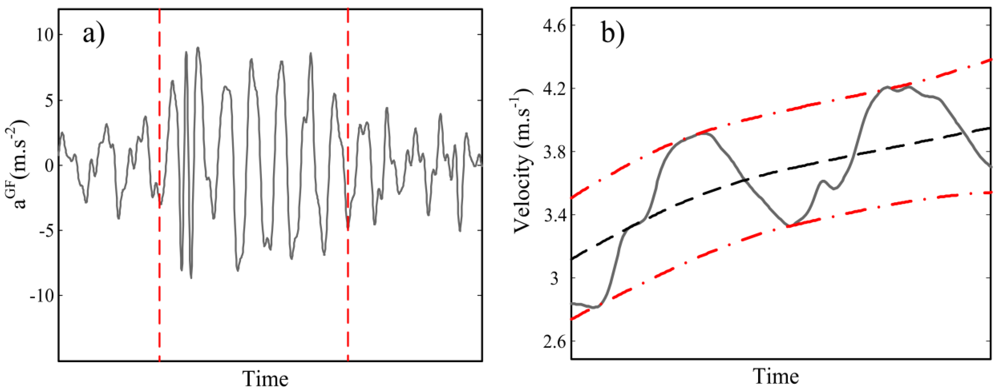
We used the geometric moving average (GMA) change detection algorithm [<xref ref-type="bibr" rid="b21-sensors-12-12927">21</xref>] for 
<inline-formula>
<mml:math id="mm18" display="inline">
<mml:semantics id="sm18">
<mml:mrow>
<mml:msubsup>
<mml:mi>a</mml:mi>
<mml:mi>t</mml:mi>
<mml:mi>Y</mml:mi></mml:msubsup></mml:mrow></mml:semantics></mml:math></inline-formula> segmentation. The algorithm is based on recursive estimation of signal variance and detecting if the variance change exceeds a predefined threshold. The threshold was selected empirically as 20% of the 
<inline-formula>
<mml:math id="mm19" display="inline">
<mml:semantics id="sm19">
<mml:mrow>
<mml:msubsup>
<mml:mi>a</mml:mi>
<mml:mi>t</mml:mi>
<mml:mi>Y</mml:mi></mml:msubsup></mml:mrow></mml:semantics></mml:math></inline-formula> variance. Much smaller thresholds end up to detection of spurious signal segments while higher thresholds cannot recognize any changes of swimming regime. <xref ref-type="fig" rid="f3-sensors-12-12927">Figure 3(a)</xref> illustrates the result of this segmentation.</p>
<p>For velocity drift removal, we assumed the average trend of <italic>V<sub>t</sub></italic> peaks within each segment is quasi-constant due to the steady regime of swimming. Therefore, at each segment, cycle minimum and maximum peaks of <italic>V<sub>t</sub></italic> were extracted and a shape preserving spline [<xref ref-type="bibr" rid="b22-sensors-12-12927">22</xref>] was fitted to these peaks [<xref ref-type="bibr" rid="b23-sensors-12-12927">23</xref>].</p>
<p>De-trending was done by subtracting the average of upper and lower trend curves from the original velocity curve. <xref ref-type="fig" rid="f3-sensors-12-12927">Figure 3(b)</xref> depicts the extraction of the trend pattern. The instantaneous velocity curve then will be corrected for trial mean velocity by assuming that the average velocity of the trial is known from length of the pool and the duration of each trial. Finally, <italic>V̄<sub>Ck</sub></italic> was estimated as the mean value of <italic>V<sub>t</sub></italic> for each cycle <italic>C<sub>k</sub></italic>. The algorithm development phase was completed by using the data of only 10 swimmers and then our algorithm was applied to the entire data set (30 swimmers).</p></sec>
<sec sec-type="methods">
<label>2.5.</label>
<title>Statistical Analysis</title>
<p>A twofold validation of the proposed velocity estimation method is presented in this section. In the first step, we provided the statistics to assess the cycle mean velocity estimated using our system 
<inline-formula>
<mml:math id="mm20" display="inline">
<mml:semantics id="sm20">
<mml:mrow>
<mml:mo stretchy="false">(</mml:mo>
<mml:msubsup>
<mml:mover accent="true">
<mml:mi>V</mml:mi>
<mml:mo>¯</mml:mo></mml:mover>
<mml:mrow>
<mml:msub>
<mml:mi>C</mml:mi>
<mml:mi>k</mml:mi></mml:msub></mml:mrow>
<mml:mrow>
<mml:mtext mathvariant="italic">IMU</mml:mtext></mml:mrow></mml:msubsup>
<mml:mo stretchy="false">)</mml:mo></mml:mrow></mml:semantics></mml:math></inline-formula>. To this end, the mean (accuracy) and standard deviation (precision) of the difference between
<inline-formula>
<mml:math id="mm21" display="inline">
<mml:semantics id="sm21">
<mml:mrow>
<mml:msubsup>
<mml:mover accent="true">
<mml:mi>V</mml:mi>
<mml:mo>¯</mml:mo></mml:mover>
<mml:mrow>
<mml:msub>
<mml:mi>C</mml:mi>
<mml:mi>k</mml:mi></mml:msub></mml:mrow>
<mml:mrow>
<mml:mtext mathvariant="italic">SRT</mml:mtext></mml:mrow></mml:msubsup></mml:mrow></mml:semantics></mml:math></inline-formula> measured by SpeedRT system and obtained from IMU, 
<inline-formula>
<mml:math id="mm22" display="inline">
<mml:semantics id="sm22">
<mml:mrow>
<mml:msubsup>
<mml:mover accent="true">
<mml:mi>V</mml:mi>
<mml:mo>¯</mml:mo></mml:mover>
<mml:mrow>
<mml:msub>
<mml:mi>C</mml:mi>
<mml:mi>k</mml:mi></mml:msub></mml:mrow>
<mml:mrow>
<mml:mtext mathvariant="italic">IMU</mml:mtext></mml:mrow></mml:msubsup></mml:mrow></mml:semantics></mml:math></inline-formula>, was calculated for different trials of each subject. Spearman's rank correlation was also used to verify the association between the two systems. Agreement between the two systems in <italic>V̄<sub>Ck</sub></italic> measurement was assessed by use of Bland-Altman plot [<xref ref-type="bibr" rid="b24-sensors-12-12927">24</xref>] and normalized pairwise variability index (nPVI) [<xref ref-type="bibr" rid="b25-sensors-12-12927">25</xref>] as calculated by <xref rid="FD11" ref-type="disp-formula">Equation (11)</xref>:
<disp-formula id="FD11">
<label>(11)</label>
<mml:math id="mm23" display="block">
<mml:semantics id="sm23">
<mml:mrow>
<mml:mi>n</mml:mi>
<mml:mi>P</mml:mi>
<mml:mi>V</mml:mi>
<mml:mi>I</mml:mi>
<mml:mo>=</mml:mo>
<mml:mn>100</mml:mn>
<mml:mo>%</mml:mo>
<mml:mo>×</mml:mo>
<mml:mrow>
<mml:mo>[</mml:mo>
<mml:mrow>
<mml:mrow>
<mml:mrow>
<mml:munderover>
<mml:mo>∑</mml:mo>
<mml:mrow>
<mml:msub>
<mml:mi>C</mml:mi>
<mml:mi>k</mml:mi></mml:msub>
<mml:mo>=</mml:mo>
<mml:mn>1</mml:mn></mml:mrow>
<mml:mi>N</mml:mi></mml:munderover>
<mml:mrow>
<mml:mrow>
<mml:mo>|</mml:mo>
<mml:mrow>
<mml:mfrac>
<mml:mrow>
<mml:msubsup>
<mml:mover accent="true">
<mml:mi>V</mml:mi>
<mml:mo>¯</mml:mo></mml:mover>
<mml:mrow>
<mml:msub>
<mml:mi>C</mml:mi>
<mml:mi>k</mml:mi></mml:msub></mml:mrow>
<mml:mrow>
<mml:mtext mathvariant="italic">SRT</mml:mtext></mml:mrow></mml:msubsup>
<mml:mo>−</mml:mo>
<mml:msubsup>
<mml:mover accent="true">
<mml:mi>V</mml:mi>
<mml:mo>¯</mml:mo></mml:mover>
<mml:mrow>
<mml:msub>
<mml:mi>C</mml:mi>
<mml:mi>k</mml:mi></mml:msub></mml:mrow>
<mml:mrow>
<mml:mtext mathvariant="italic">IMU</mml:mtext></mml:mrow></mml:msubsup></mml:mrow>
<mml:mrow>
<mml:mrow>
<mml:mrow>
<mml:mrow>
<mml:mo>(</mml:mo>
<mml:mrow>
<mml:msubsup>
<mml:mover accent="true">
<mml:mi>V</mml:mi>
<mml:mo>¯</mml:mo></mml:mover>
<mml:mrow>
<mml:msub>
<mml:mi>C</mml:mi>
<mml:mi>k</mml:mi></mml:msub></mml:mrow>
<mml:mrow>
<mml:mtext mathvariant="italic">SRT</mml:mtext></mml:mrow></mml:msubsup>
<mml:mo>+</mml:mo>
<mml:msubsup>
<mml:mover accent="true">
<mml:mi>V</mml:mi>
<mml:mo>¯</mml:mo></mml:mover>
<mml:mrow>
<mml:msub>
<mml:mi>C</mml:mi>
<mml:mi>k</mml:mi></mml:msub></mml:mrow>
<mml:mrow>
<mml:mtext mathvariant="italic">IMU</mml:mtext></mml:mrow></mml:msubsup></mml:mrow>
<mml:mo>)</mml:mo></mml:mrow></mml:mrow>
<mml:mo stretchy="true">/</mml:mo>
<mml:mn>2</mml:mn></mml:mrow></mml:mrow></mml:mfrac></mml:mrow>
<mml:mo>|</mml:mo></mml:mrow></mml:mrow></mml:mrow>
<mml:mo stretchy="true">/</mml:mo>
<mml:mi>N</mml:mi></mml:mrow></mml:mrow>
<mml:mo>]</mml:mo></mml:mrow></mml:mrow></mml:semantics></mml:math></disp-formula>where <italic>N</italic> is the total number of studied cycles. The Bland-Altman plot was inspected with correlation exploration for existence of heteroscedasticity [<xref ref-type="bibr" rid="b26-sensors-12-12927">26</xref>].</p>
<p>In the second step we investigated the efficiency of our method in measuring the instantaneous velocity. The root mean squared (RMS), maximum and corresponding relative error of instantaneous velocity was calculated. As these calculations require similar time sampling of proposed and reference systems, the instantaneous velocity curve calculated by our method was downsampled to 100 Hz prior to error calculations. Besides, an indirect measure of accuracy of our system in instantaneous velocity measurement was provided by assessment of intra-cyclic velocity variation (IVV). In fact, the concurrent validity of our method was assessed by investigating IVV of the two groups of swimmers (Elite and Recreational), estimated by the two systems. IVV is computed as in <xref rid="FD12" ref-type="disp-formula">Equation (12)</xref>:
<disp-formula id="FD12">
<label>(12)</label>
<mml:math id="mm24" display="block">
<mml:semantics id="sm24">
<mml:mrow>
<mml:mtext mathvariant="italic">IVV</mml:mtext>
<mml:mo>=</mml:mo>
<mml:mfrac>
<mml:mrow>
<mml:msqrt>
<mml:mrow>
<mml:munderover>
<mml:mtext>∑</mml:mtext>
<mml:mrow>
<mml:msub>
<mml:mi>C</mml:mi>
<mml:mi>k</mml:mi></mml:msub>
<mml:mo>=</mml:mo>
<mml:mn>1</mml:mn></mml:mrow>
<mml:mi>C</mml:mi></mml:munderover>
<mml:mrow>
<mml:munder>
<mml:mtext>∑</mml:mtext>
<mml:mrow>
<mml:msub>
<mml:mi>C</mml:mi>
<mml:mi>k</mml:mi></mml:msub>
<mml:mo>≤</mml:mo>
<mml:mi>t</mml:mi>
<mml:mo>&lt;</mml:mo>
<mml:msub>
<mml:mi>C</mml:mi>
<mml:mrow>
<mml:mi>k</mml:mi>
<mml:mo>+</mml:mo>
<mml:mn>1</mml:mn></mml:mrow></mml:msub></mml:mrow></mml:munder>
<mml:mrow>
<mml:msup>
<mml:mrow>
<mml:mrow>
<mml:mo>(</mml:mo>
<mml:mrow>
<mml:msub>
<mml:mi>V</mml:mi>
<mml:mi>t</mml:mi></mml:msub>
<mml:mo>−</mml:mo>
<mml:msub>
<mml:mover accent="true">
<mml:mi>V</mml:mi>
<mml:mo>¯</mml:mo></mml:mover>
<mml:mrow>
<mml:msub>
<mml:mi>C</mml:mi>
<mml:mi>k</mml:mi></mml:msub></mml:mrow></mml:msub></mml:mrow>
<mml:mo>)</mml:mo></mml:mrow></mml:mrow>
<mml:mn>2</mml:mn></mml:msup>
<mml:mrow>
<mml:mrow>
<mml:msub>
<mml:mi>f</mml:mi>
<mml:mrow>
<mml:msub>
<mml:mi>C</mml:mi>
<mml:mi>k</mml:mi></mml:msub></mml:mrow></mml:msub></mml:mrow>
<mml:mo stretchy="true">/</mml:mo>
<mml:mi>n</mml:mi></mml:mrow></mml:mrow></mml:mrow></mml:mrow></mml:msqrt></mml:mrow>
<mml:mrow>
<mml:munderover>
<mml:mtext>∑</mml:mtext>
<mml:mrow>
<mml:msub>
<mml:mi>C</mml:mi>
<mml:mi>k</mml:mi></mml:msub>
<mml:mo>=</mml:mo>
<mml:mn>1</mml:mn></mml:mrow>
<mml:mi>C</mml:mi></mml:munderover>
<mml:mrow>
<mml:munder>
<mml:mtext>∑</mml:mtext>
<mml:mrow>
<mml:msub>
<mml:mi>C</mml:mi>
<mml:mi>k</mml:mi></mml:msub>
<mml:mo>≤</mml:mo>
<mml:mi>t</mml:mi>
<mml:mo>&lt;</mml:mo>
<mml:msub>
<mml:mi>C</mml:mi>
<mml:mrow>
<mml:mi>k</mml:mi>
<mml:mo>+</mml:mo>
<mml:mn>1</mml:mn></mml:mrow></mml:msub></mml:mrow></mml:munder>
<mml:mrow>
<mml:msub>
<mml:mi>V</mml:mi>
<mml:mi>t</mml:mi></mml:msub>
<mml:mspace width="0.4em"/>
<mml:mrow>
<mml:mrow>
<mml:msub>
<mml:mi>f</mml:mi>
<mml:mrow>
<mml:msub>
<mml:mi>C</mml:mi>
<mml:mi>k</mml:mi></mml:msub></mml:mrow></mml:msub></mml:mrow>
<mml:mo stretchy="true">/</mml:mo>
<mml:mi>n</mml:mi></mml:mrow></mml:mrow></mml:mrow></mml:mrow></mml:mfrac></mml:mrow></mml:semantics></mml:math></disp-formula>where <italic>f<sub>Ck</sub></italic> represents cycle frequency, <italic>C</italic> is the number of cycles in the trial and <italic>n</italic> is the number of trial samples [<xref ref-type="bibr" rid="b27-sensors-12-12927">27</xref>]. We performed a three-way repeated ANOVA (significance level of <italic>p</italic> &lt; 0.01) to examine the effect of trial, group and measurement device on IVV.</p></sec></sec>
<sec sec-type="results|discussion">
<label>3.</label>
<title>Results and Discussion</title>
<p>
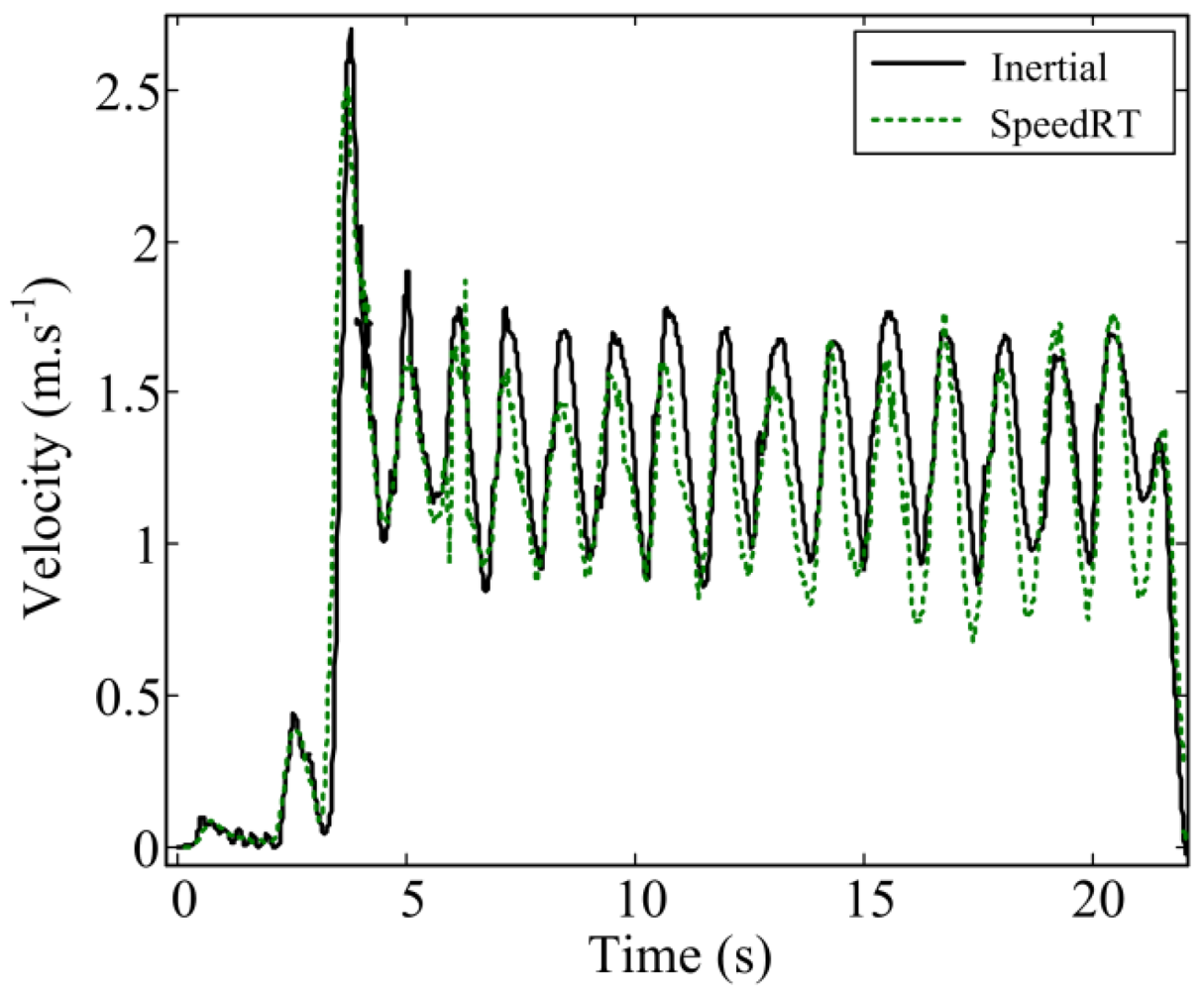
We have proposed a new wearable system and dedicated algorithms to measure front crawl velocity and described its validation procedure against a reference tethered device. <xref ref-type="fig" rid="f4-sensors-12-12927">Figure 4</xref> illustrates a typical result of the instantaneous velocity obtained with our method and the reference system. A total number of N = 1,448 cycles were compared between the two systems.</p>
<p>A significant correlation was observed between the two systems (Spearman's <italic>rho</italic> = <italic>0.94</italic>, <italic>p</italic> &lt; <italic>0.001</italic>) in <italic>V̄<sub>Ck</sub></italic> assessment. The 
<inline-formula>
<mml:math id="mm25" display="inline">
<mml:semantics id="sm25">
<mml:mrow>
<mml:msubsup>
<mml:mover accent="true">
<mml:mi>V</mml:mi>
<mml:mo>¯</mml:mo></mml:mover>
<mml:mrow>
<mml:msub>
<mml:mi>C</mml:mi>
<mml:mi>k</mml:mi></mml:msub></mml:mrow>
<mml:mrow>
<mml:mtext mathvariant="italic">IMU</mml:mtext></mml:mrow></mml:msubsup></mml:mrow></mml:semantics></mml:math></inline-formula> and the 
<inline-formula>
<mml:math id="mm26" display="inline">
<mml:semantics id="sm26">
<mml:mrow>
<mml:msubsup>
<mml:mover accent="true">
<mml:mi>V</mml:mi>
<mml:mo>¯</mml:mo></mml:mover>
<mml:mrow>
<mml:msub>
<mml:mi>C</mml:mi>
<mml:mi>k</mml:mi></mml:msub></mml:mrow>
<mml:mrow>
<mml:mtext mathvariant="italic">SRT</mml:mtext></mml:mrow></mml:msubsup></mml:mrow></mml:semantics></mml:math></inline-formula> differed by 0.6 cm·s<sup>−1</sup> and the precision was 5.4 cm·s<sup>−1</sup> 
<inline-formula>
<mml:math id="mm27" display="inline">
<mml:semantics id="sm27">
<mml:mrow>
<mml:mo stretchy="false">(</mml:mo>
<mml:msubsup>
<mml:mover accent="true">
<mml:mi>V</mml:mi>
<mml:mo>¯</mml:mo></mml:mover>
<mml:mrow>
<mml:msub>
<mml:mi>C</mml:mi>
<mml:mi>k</mml:mi></mml:msub></mml:mrow>
<mml:mrow>
<mml:mtext mathvariant="italic">SRT</mml:mtext></mml:mrow></mml:msubsup></mml:mrow></mml:semantics></mml:math></inline-formula> range [0.91, 1.95] cm.s<sup>−1</sup>). <xref ref-type="table" rid="t2-sensors-12-12927">Table 2</xref> summarizes the <italic>V̄<sub>Ck</sub></italic> comparison between the two systems for all four different ranges of mean velocity (as measured by the reference and IMU). The results demonstrate that the proposed system is capable of measuring front-crawl velocity with acceptable accuracy (below 1.1 cm·s<sup>−1</sup>) and precision (below 5.8 cm·s<sup>−1</sup>) suggesting that our method can be reliably used for cycle mean velocity measurements. This accurate estimation of stroke cycle velocity was possible thanks to: (i) sensor orientation drift removal in <italic>GF</italic> using the principal component of swimming kinematics; (ii) velocity drift removal by introducing an appropriate segmentation of forward acceleration and by a spline shape modeling of the drift at each segment after integration of acceleration.</p>
<p>The two systems differed by 3.5% in assessment of <italic>V̄<sub>Ck</sub></italic> variations as presented by nPVI in <xref ref-type="table" rid="t2-sensors-12-12927">Table 2</xref>. The nPVI values in <xref ref-type="table" rid="t2-sensors-12-12927">Table 2</xref> shows that the difference in variability assessment of <italic>V̄<sub>Ck</sub></italic> between the two systems in four ranges of velocity is less than 3.9%. This result as well as high <italic>V̄<sub>Ck</sub></italic> correlation between the two systems confirms that our method detects the <italic>V̄<sub>Ck</sub></italic> changes similar to the reference and supports the validity of our estimation.</p>
<p>
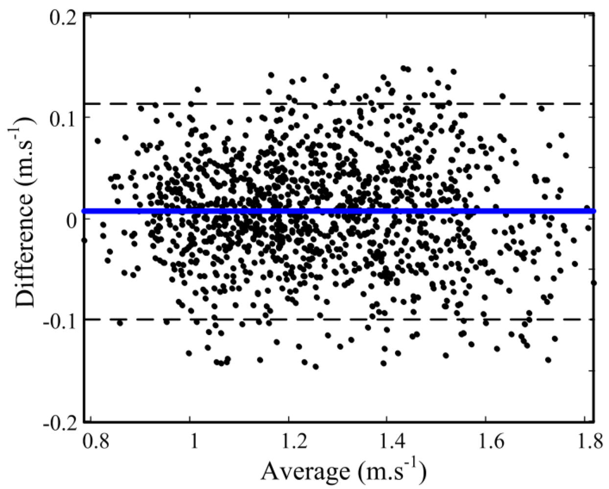
The Bland–Altman plot showed the 95% limits of agreement lower than 10.8 cm·s<sup>−1</sup> between the two systems in <italic>V̄<sub>Ck</sub></italic> assessment as depicted in <xref ref-type="fig" rid="f5-sensors-12-12927">Figure 5</xref>, where no significant difference and no heteroscedasticity (correlation = 0.03) were found. This finding, implies uniform performance of the method throughout the studied range of <italic>V̄<sub>Ck</sub></italic>. It is noteworthy that by using the prior information about pool length to correct the velocity profile an error of 10.4 ± 39.7 cm is observed in estimating the sacrum's displacement. This error was expected since the sacrum does not necessarily travel a complete length of the swimming pool.</p>
<p>As regards validation of instantaneous velocity, an RMS difference of 11.3 cm·s<sup>−1</sup> was observed that is comparable to the precision of the reference system. The maximum instantaneous error was 18.2 cm·s<sup>−1</sup> that corresponds to a relative error of 9.7%. One source of the difference between the velocity estimated by our method and the velocity measured by the reference is a small artifact due to the non-rigidness of the swimming suit. Nevertheless, the custom designed swimming suit used to fix the sensor did not allow the sensor to move drastically and kept the artifact within a tolerable range. Moreover, during high accelerations when the artifact is more pronounced, the random bias of accelerometer is less significant (higher signal to noise ratio) which leads to acceptable results [<xref ref-type="bibr" rid="b28-sensors-12-12927">28</xref>].</p>
<p>Indirect validation of instantaneous velocity by IVV in <xref ref-type="table" rid="t3-sensors-12-12927">Table 3</xref> through four different velocity ranges and the two different groups of participants, suggests that the IMU can be used for the study of instantaneous velocity variations. Indeed, our system, in accordance with the reference, showed a significant difference (<italic>p</italic> &lt; 0.01, <italic>p</italic> &lt; 0.001) to discriminate elite and recreational group based on IVV values (in different ranges of velocity). The reference showed an IVV change from 13.7% to 17.5% for the elite group and from 19.6% to 23.3% for the recreational group. Our method in accordance with the reference, showed significantly lower IVV values for elite swimmers (<xref ref-type="table" rid="t3-sensors-12-12927">Table 3</xref>) that is consistent with previous studies [<xref ref-type="bibr" rid="b7-sensors-12-12927">7</xref>,<xref ref-type="bibr" rid="b29-sensors-12-12927">29</xref>].</p>
<p>Another observation from <xref ref-type="table" rid="t3-sensors-12-12927">Table 3</xref> is that the IMU tends to underestimate the IVV as presented by positive error values. However, the ANOVA shows that the small systematic difference between the two systems is not affected by group factor (<italic>p</italic> &gt; 0.3). In a nutshell, using IMU the same systematic error can be seen for different groups of swimmers and can be compensated.</p>
<p>The ability of the inertial sensor to distinguish the variability of the movement of the subjects with different performance levels propounds the application of the inertial system in the study of swimming velocity. The capacity of our system to detect IVV changes also provides important evidence that our velocity drift removal method does not cancel out the velocity variations. Indeed, different swimming trial regimes were recognized based on changes of acceleration magnitude. These regimes are treated separately to mitigate the effect of the velocity drift and thereof variation of velocity signal was well maintained.</p>
<p>Signal segmentation using GMA is the core of drift removal in our method. Therefore, investigating the effect of changing the segmentation threshold in GMA can be illustrative of the method's robustness. To this end, the threshold in the GMA algorithm was shifted 5%. The effect of this change on the estimation is shown in <xref ref-type="table" rid="t4-sensors-12-12927">Table 4</xref>. It can be seen that a decrement of 5% in the threshold led to a bigger error in the estimated velocity than equal increment. The small threshold caused many spurious segments on the 
<inline-formula>
<mml:math id="mm28" display="inline">
<mml:semantics id="sm28">
<mml:mrow>
<mml:msubsup>
<mml:mi>a</mml:mi>
<mml:mi>t</mml:mi>
<mml:mi>Y</mml:mi></mml:msubsup></mml:mrow></mml:semantics></mml:math></inline-formula> signal which resulted in excessive localized correction on the velocity pattern; on the contrary, since during 25 m laps the actual acceleration profile of the swimmers does not change frequently, the higher threshold did not notably cut down on the algorithm performance.</p>
<p>Our dataset includes only one type of initial condition (swimming starts from a relatively motionless posture in water followed by a wall push) that is a subset of possible initial conditions in swimming. However, the study of other initial condition was not feasible within the scope of our experiment for practical reasons. Since the tethered reference only measures the velocity in forward direction of swimming, comparison of the multi lap data with turns between the IMU and the tethered device was not realizable. Although diving from the start block was a possibility, we avoided it for two practical considerations. Firstly, during the diving period calculation of the parallax effect on the velocity measured by the tethered reference is not possible. Secondly, avoiding the dives we could collect more stroke cycles which augments the statistical power of our study.</p>
<p>The algorithm we proposed in this paper, despite providing timely results, should not be misinterpreted as being real time. The data stream of one complete lap serves as the input of our algorithm since the correction is performed per lap. For a near real-time implementation of our method a crucial step is to determine the cycle mean velocity without using prior information about pool length.</p></sec>
<sec sec-type="conclusions">
<label>4.</label>
<title>Conclusions</title>
<p>The proposed method presents a reliable IMU-based system that can be practically used to measure the swimming velocity as the most intuitive metric of the athlete's performance. The system is user-centric meaning that several athletes can wear their own sensor at a time without interfering with the other athletes' measurements. Development of such a tool can help coaches pinpoint the strengths and weaknesses of the athletes during workout sessions and design an optimal personal training plan for athletes to improve their performance.</p>
<p>Accurate measurement of swimming velocity allowed the assessment of intra-cycle variability, an important determinant of swimming efficiency. Analysis of swimming velocity along with other parameters such as coordination [<xref ref-type="bibr" rid="b11-sensors-12-12927">11</xref>] and energy expenditure can shed a new light on the biomechanics of locomotion in water. Further studies towards developing signal processing techniques for accurate assessment of velocity in the other swimming strokes are required. Estimation of cycle mean velocity independent of pool length information is also an interesting open problem in the future perspective of the study.</p></sec></body>
<back>
<ack>
<p>The authors wish to thank Arash Salarian for his technical advice. The work was supported by Swiss National Science Foundation (SNSF), grant No. 320030-127554.</p></ack>
<ref-list>
<title>References</title>
<ref id="b1-sensors-12-12927"><label>1.</label><citation citation-type="journal"><person-group person-group-type="author"><name><surname>Puel</surname><given-names>F.</given-names></name><name><surname>Morlier</surname><given-names>J.</given-names></name><name><surname>Avalos</surname><given-names>M.</given-names></name><name><surname>Mesnard</surname><given-names>M.</given-names></name><name><surname>Cid</surname><given-names>M.</given-names></name><name><surname>Hellard</surname><given-names>P.</given-names></name></person-group><article-title>3D kinematic and dynamic analysis of the front crawl tumble turn in elite male swimmers</article-title><source>J. Biomech.</source><year>2012</year><volume>45</volume><fpage>510</fpage><lpage>515</lpage><pub-id pub-id-type="doi">10.1016/j.jbiomech.2011.11.043</pub-id><pub-id pub-id-type="pmid">22176710</pub-id></citation></ref>
<ref id="b2-sensors-12-12927"><label>2.</label><citation citation-type="journal"><person-group person-group-type="author"><name><surname>Vezos</surname><given-names>N.</given-names></name><name><surname>Gourgoulis</surname><given-names>V.</given-names></name><name><surname>Aggeloussis</surname><given-names>N.</given-names></name><name><surname>Kasimatis</surname><given-names>P.</given-names></name><name><surname>Christoforidis</surname><given-names>C.</given-names></name><name><surname>Mavromatis</surname><given-names>G.</given-names></name></person-group><article-title>Underwater stroke kinematics during breathing and breath-holding front crawl swimming</article-title><source>J. Sport Sci. Med.</source><year>2007</year><volume>6</volume><fpage>58</fpage><lpage>62</lpage></citation></ref>
<ref id="b3-sensors-12-12927"><label>3.</label><citation citation-type="journal"><person-group person-group-type="author"><name><surname>Callaway</surname><given-names>A.J.</given-names></name><name><surname>Cobb</surname><given-names>J.E.</given-names></name><name><surname>Jones</surname><given-names>I.</given-names></name></person-group><article-title>A comparison of video and accelerometer based approaches applied to performance monitoring in swimming</article-title><source>Int. J. Sports Sci. Coach.</source><year>2009</year><volume>4</volume><fpage>139</fpage><lpage>153</lpage><pub-id pub-id-type="doi">10.1260/1747-9541.4.1.139</pub-id></citation></ref>
<ref id="b4-sensors-12-12927"><label>4.</label><citation citation-type="journal"><person-group person-group-type="author"><name><surname>Ceseracciu</surname><given-names>E.</given-names></name><name><surname>Sawacha</surname><given-names>Z.</given-names></name><name><surname>Fantozzi</surname><given-names>S.</given-names></name><name><surname>Cortesi</surname><given-names>M.</given-names></name><name><surname>Gatta</surname><given-names>G.</given-names></name><name><surname>Corazza</surname><given-names>S.</given-names></name><name><surname>Cobelli</surname><given-names>C.</given-names></name></person-group><article-title>Markerless analysis of front crawl swimming</article-title><source>J. Biomech.</source><year>2011</year><volume>44</volume><fpage>2236</fpage><lpage>2242</lpage><pub-id pub-id-type="doi">10.1016/j.jbiomech.2011.06.003</pub-id><pub-id pub-id-type="pmid">21719017</pub-id></citation></ref>
<ref id="b5-sensors-12-12927"><label>5.</label><citation citation-type="confproc"><person-group person-group-type="author"><name><surname>Plaenkers</surname><given-names>R.</given-names></name><name><surname>Fua</surname><given-names>P.</given-names></name></person-group><article-title>Model-Based Silhouette Extraction for Accurate People Tracking</article-title><conf-name>Proceedings of European Conference on Computer Vision</conf-name><conf-loc>Copenhagen, Denmark</conf-loc><conf-date>28–31 May 2002</conf-date><fpage>325</fpage><lpage>339</lpage></citation></ref>
<ref id="b6-sensors-12-12927"><label>6.</label><citation citation-type="journal"><person-group person-group-type="author"><name><surname>Craig</surname><given-names>A.B.</given-names></name><name><surname>Termin</surname><given-names>B.</given-names></name><name><surname>Pendergast</surname><given-names>D.R.</given-names></name></person-group><article-title>Simultaneous recordings of velocity and video during swimming</article-title><source>Port. J. Sport Sci.</source><year>2006</year><volume>6</volume><fpage>32</fpage><lpage>35</lpage></citation></ref>
<ref id="b7-sensors-12-12927"><label>7.</label><citation citation-type="journal"><person-group person-group-type="author"><name><surname>Schnitzler</surname><given-names>C.</given-names></name><name><surname>Seifert</surname><given-names>L.</given-names></name><name><surname>Alberty</surname><given-names>M.</given-names></name><name><surname>Chollet</surname><given-names>D.</given-names></name></person-group><article-title>Hip velocity and arm coordination in front crawl swimming</article-title><source>Int. J. Sports Med.</source><year>2010</year><volume>31</volume><fpage>875</fpage><lpage>881</lpage><pub-id pub-id-type="doi">10.1055/s-0030-1265149</pub-id><pub-id pub-id-type="pmid">21072734</pub-id></citation></ref>
<ref id="b8-sensors-12-12927"><label>8.</label><citation citation-type="journal"><person-group person-group-type="author"><name><surname>Justham</surname><given-names>L.</given-names></name><name><surname>Slawson</surname><given-names>S.</given-names></name><name><surname>West</surname><given-names>A.</given-names></name><name><surname>Conway</surname><given-names>P.</given-names></name><name><surname>Caine</surname><given-names>M.</given-names></name><name><surname>Harrison</surname><given-names>R.</given-names></name></person-group><article-title>Enabling Technologies for Robust Performance Monitoring (P10)</article-title><source>Eng. Sport</source><year>2008</year><volume>7</volume><fpage>45</fpage><lpage>54</lpage></citation></ref>
<ref id="b9-sensors-12-12927"><label>9.</label><citation citation-type="journal"><person-group person-group-type="author"><name><surname>Yang</surname><given-names>S.</given-names></name><name><surname>Li</surname><given-names>Q.</given-names></name></person-group><article-title>Inertial sensor-based methods in walking speed estimation: A systematic review</article-title><source>Sensors</source><year>2012</year><volume>12</volume><fpage>6102</fpage><lpage>6116</lpage><pub-id pub-id-type="doi">10.3390/s120506102</pub-id><pub-id pub-id-type="pmid">22778632</pub-id></citation></ref>
<ref id="b10-sensors-12-12927"><label>10.</label><citation citation-type="journal"><person-group person-group-type="author"><name><surname>Marsland</surname><given-names>F.</given-names></name><name><surname>Lyons</surname><given-names>K.</given-names></name><name><surname>Anson</surname><given-names>J.</given-names></name><name><surname>Waddington</surname><given-names>G.</given-names></name><name><surname>Macintosh</surname><given-names>C.</given-names></name><name><surname>Chapman</surname><given-names>D.</given-names></name></person-group><article-title>Identification of cross-country skiing movement patterns using micro-sensors</article-title><source>Sensors</source><year>2012</year><volume>12</volume><fpage>5047</fpage><lpage>5066</lpage><pub-id pub-id-type="doi">10.3390/s120405047</pub-id><pub-id pub-id-type="pmid">22666075</pub-id></citation></ref>
<ref id="b11-sensors-12-12927"><label>11.</label><citation citation-type="journal"><person-group person-group-type="author"><name><surname>Dadashi</surname><given-names>F.</given-names></name><name><surname>Crettenand</surname><given-names>F.</given-names></name><name><surname>Millet</surname><given-names>G.</given-names></name><name><surname>Seifert</surname><given-names>L.</given-names></name><name><surname>Komar</surname><given-names>J.</given-names></name><name><surname>Aminian</surname><given-names>K.</given-names></name></person-group><article-title>Front Crawl Propulsive Phase Detection Using Inertial Sensors</article-title><source>Port. J. Sport Sci.</source><year>2011</year><volume>11</volume><fpage>855</fpage><lpage>858</lpage></citation></ref>
<ref id="b12-sensors-12-12927"><label>12.</label><citation citation-type="journal"><person-group person-group-type="author"><name><surname>Ayrulu-Erdem</surname><given-names>B.</given-names></name><name><surname>Barshan</surname><given-names>B.</given-names></name></person-group><article-title>Leg motion classification with artificial neural networks using wavelet-based features of gyroscope signals</article-title><source>Sensors</source><year>2011</year><volume>11</volume><fpage>1721</fpage><lpage>1743</lpage><pub-id pub-id-type="doi">10.3390/s110201721</pub-id><pub-id pub-id-type="pmid">22319378</pub-id></citation></ref>
<ref id="b13-sensors-12-12927"><label>13.</label><citation citation-type="journal"><person-group person-group-type="author"><name><surname>Ohgi</surname><given-names>Y.</given-names></name></person-group><article-title>Microcomputer-based Acceleration Sensor Device for Sports Biomechanics—Stroke Evaluation by using Swimmers Wrist Acceleration</article-title><source>Sensors</source><year>2002</year><volume>1</volume><fpage>699</fpage><lpage>704</lpage></citation></ref>
<ref id="b14-sensors-12-12927"><label>14.</label><citation citation-type="journal"><person-group person-group-type="author"><name><surname>Davey</surname><given-names>N.</given-names></name><name><surname>Anderson</surname><given-names>M.</given-names></name><name><surname>James</surname><given-names>D.A.</given-names></name></person-group><article-title>Validation trial of an accelerometer-based sensor platform for swimming</article-title><source>Sports Technol.</source><year>2008</year><volume>1</volume><fpage>202</fpage><lpage>207</lpage><pub-id pub-id-type="doi">10.1002/jst.59</pub-id></citation></ref>
<ref id="b15-sensors-12-12927"><label>15.</label><citation citation-type="journal"><person-group person-group-type="author"><name><surname>Le Sage</surname><given-names>T.</given-names></name><name><surname>Bindel</surname><given-names>A.</given-names></name><name><surname>Conway</surname><given-names>P.P.</given-names></name><name><surname>Justham</surname><given-names>L.M.</given-names></name><name><surname>Slawson</surname><given-names>S.E.</given-names></name><name><surname>West</surname><given-names>A.A.</given-names></name></person-group><article-title>Embedded programming and real-time signal processing of swimming strokes</article-title><source>Sports Eng.</source><year>2011</year><volume>14</volume><fpage>1</fpage><lpage>14</lpage><pub-id pub-id-type="doi">10.1007/s12283-011-0070-7</pub-id></citation></ref>
<ref id="b16-sensors-12-12927"><label>16.</label><citation citation-type="confproc"><person-group person-group-type="author"><name><surname>Stamm</surname><given-names>A.</given-names></name><name><surname>Thiel</surname><given-names>D.V.</given-names></name><name><surname>Burkett</surname><given-names>B.</given-names></name><name><surname>James</surname><given-names>D.A.</given-names></name></person-group><article-title>Towards Determining Absolute Velocity of Freestyle Swimming Using 3-Axis Accelerometers</article-title><conf-name>Proceedings of the 5th Asia-Pacific Congress on Sports Technology</conf-name><conf-loc>Melbourne, Australia</conf-loc><conf-date>28–31 August 2011</conf-date><volume>13</volume><fpage>120</fpage><lpage>125</lpage></citation></ref>
<ref id="b17-sensors-12-12927"><label>17.</label><citation citation-type="book"><person-group person-group-type="author"><name><surname>Titterton</surname><given-names>D.H.</given-names></name><name><surname>Weston</surname><given-names>J.L.</given-names></name></person-group><source>Strapdown Inertial Navigation Technology</source><publisher-name>Peter Peregrinus Ltd.</publisher-name><publisher-loc>London, UK</publisher-loc><year>2004</year></citation></ref>
<ref id="b18-sensors-12-12927"><label>18.</label><citation citation-type="journal"><person-group person-group-type="author"><name><surname>Ferraris</surname><given-names>F.</given-names></name><name><surname>Grimaldi</surname><given-names>U.</given-names></name><name><surname>Parvis</surname><given-names>M.</given-names></name></person-group><article-title>Procedure for effortless in-field calibration of three-axis rate gyros and accelerometers</article-title><source>Sens. Mater.</source><year>1995</year><volume>7</volume><fpage>311</fpage><lpage>330</lpage></citation></ref>
<ref id="b19-sensors-12-12927"><label>19.</label><citation citation-type="journal"><person-group person-group-type="author"><name><surname>Tella</surname><given-names>V.</given-names></name><name><surname>Toca-Herrera</surname><given-names>J.L.</given-names></name><name><surname>Gallach</surname><given-names>J.E.</given-names></name><name><surname>Benavent</surname><given-names>J.</given-names></name><name><surname>González</surname><given-names>L.M.</given-names></name><name><surname>Arellano</surname><given-names>R.</given-names></name></person-group><article-title>Effect of fatigue on the intra-cycle acceleration in front crawl swimming: A time-frequency analysis</article-title><source>J. Biomech.</source><year>2008</year><volume>41</volume><fpage>86</fpage><lpage>92</lpage><pub-id pub-id-type="doi">10.1016/j.jbiomech.2007.07.012</pub-id><pub-id pub-id-type="pmid">17714719</pub-id></citation></ref>
<ref id="b20-sensors-12-12927"><label>20.</label><citation citation-type="journal"><person-group person-group-type="author"><name><surname>Bortz</surname><given-names>J.E.</given-names></name></person-group><article-title>New mathematical formulation for strapdown inertial navigation</article-title><source>IEEE Trans. Aerosp. Electr. Syst.</source><year>1971</year><volume>AES-7</volume><fpage>61</fpage><lpage>66</lpage><pub-id pub-id-type="doi">10.1109/TAES.1971.310252</pub-id></citation></ref>
<ref id="b21-sensors-12-12927"><label>21.</label><citation citation-type="book"><person-group person-group-type="author"><name><surname>Basseville</surname><given-names>M.</given-names></name><name><surname>Nikiforov</surname><given-names>I.V.</given-names></name></person-group><source>Detection of Abrupt Changes: Theory and Application</source><publisher-name>Prentice Hall Englewood Cliffs</publisher-name><publisher-loc>New York, NY, USA</publisher-loc><year>1993</year></citation></ref>
<ref id="b22-sensors-12-12927"><label>22.</label><citation citation-type="journal"><person-group person-group-type="author"><name><surname>Fritsch</surname><given-names>F.N.</given-names></name><name><surname>Carlson</surname><given-names>R.E.</given-names></name></person-group><article-title>Monotone piecewise cubic interpolation</article-title><source>SIAM J. Numer. Anal.</source><year>1980</year><fpage>238</fpage><lpage>246</lpage></citation></ref>
<ref id="b23-sensors-12-12927"><label>23.</label><citation citation-type="journal"><person-group person-group-type="author"><name><surname>Mariani</surname><given-names>B.</given-names></name><name><surname>Hoskovec</surname><given-names>C.</given-names></name><name><surname>Rochat</surname><given-names>S.</given-names></name><name><surname>Büla</surname><given-names>C.</given-names></name><name><surname>Penders</surname><given-names>J.</given-names></name><name><surname>Aminian</surname><given-names>K.</given-names></name></person-group><article-title>3D gait assessment in young and elderly subjects using foot-worn inertial sensors</article-title><source>J. Biomech.</source><year>2010</year><volume>43</volume><fpage>2999</fpage><lpage>3006</lpage><pub-id pub-id-type="doi">10.1016/j.jbiomech.2010.07.003</pub-id><pub-id pub-id-type="pmid">20656291</pub-id></citation></ref>
<ref id="b24-sensors-12-12927"><label>24.</label><citation citation-type="journal"><person-group person-group-type="author"><name><surname>Bland</surname><given-names>J.M.</given-names></name><name><surname>Altman</surname><given-names>D.G.</given-names></name></person-group><article-title>Statistical methods for assessing agreement between two methods of clinical measurement</article-title><source>Lancet</source><year>1986</year><volume>1</volume><fpage>307</fpage><lpage>310</lpage><pub-id pub-id-type="pmid">2868172</pub-id></citation></ref>
<ref id="b25-sensors-12-12927"><label>25.</label><citation citation-type="confproc"><person-group person-group-type="author"><name><surname>Sandnes</surname><given-names>F.E.</given-names></name><name><surname>Jian</surname><given-names>H.L.</given-names></name></person-group><article-title>Pair-wise variability index: Evaluating the cognitive difficulty of using mobile text entry systems</article-title><conf-name>Proceedings of Mobile Human-Computer Interaction–Mobile HCI 2004</conf-name><conf-loc>Glasgow, UK</conf-loc><conf-date>13–16 September 2004</conf-date><fpage>25</fpage><lpage>37</lpage></citation></ref>
<ref id="b26-sensors-12-12927"><label>26.</label><citation citation-type="journal"><person-group person-group-type="author"><name><surname>Atkinson</surname><given-names>G.</given-names></name><name><surname>Nevill</surname><given-names>A.M.</given-names></name></person-group><article-title>Statistical methods for assessing measurement error (reliability) in variables relevant to sports medicine</article-title><source>Sports Med.</source><year>1998</year><volume>26</volume><fpage>217</fpage><lpage>238</lpage><pub-id pub-id-type="doi">10.2165/00007256-199826040-00002</pub-id><pub-id pub-id-type="pmid">9820922</pub-id></citation></ref>
<ref id="b27-sensors-12-12927"><label>27.</label><citation citation-type="journal"><person-group person-group-type="author"><name><surname>Barbosa</surname><given-names>T.M.</given-names></name><name><surname>Bragada</surname><given-names>J.A.</given-names></name><name><surname>Reis</surname><given-names>V.M.</given-names></name><name><surname>Marinho</surname><given-names>D.A.</given-names></name><name><surname>Carvalho</surname><given-names>C.</given-names></name><name><surname>Silva</surname><given-names>A.J.</given-names></name></person-group><article-title>Energetics and biomechanics as determining factors of swimming performance: Updating the state of the art</article-title><source>J. Sci. Med. Sport</source><year>2010</year><volume>13</volume><fpage>262</fpage><lpage>269</lpage><pub-id pub-id-type="doi">10.1016/j.jsams.2009.01.003</pub-id><pub-id pub-id-type="pmid">19409842</pub-id></citation></ref>
<ref id="b28-sensors-12-12927"><label>28.</label><citation citation-type="journal"><person-group person-group-type="author"><name><surname>Pang</surname><given-names>G.</given-names></name><name><surname>Liu</surname><given-names>H.</given-names></name></person-group><article-title>Evaluation of a low-cost MEMS accelerometer for distance measurement</article-title><source>J. Intel. Robot. Syst.: Theory Appl.</source><year>2001</year><volume>30</volume><fpage>249</fpage><lpage>265</lpage><pub-id pub-id-type="doi">10.1023/A:1008113324758</pub-id></citation></ref>
<ref id="b29-sensors-12-12927"><label>29.</label><citation citation-type="journal"><person-group person-group-type="author"><name><surname>Seifert</surname><given-names>L.</given-names></name><name><surname>Toussaint</surname><given-names>H.M.</given-names></name><name><surname>Alberty</surname><given-names>M.</given-names></name><name><surname>Schnitzler</surname><given-names>C.</given-names></name><name><surname>Chollet</surname><given-names>D.</given-names></name></person-group><article-title>Arm coordination, power, and swim efficiency in national and regional front crawl swimmers</article-title><source>Hum. Mov. Sci.</source><year>2010</year><volume>29</volume><fpage>426</fpage><lpage>439</lpage><pub-id pub-id-type="doi">10.1016/j.humov.2009.11.003</pub-id><pub-id pub-id-type="pmid">20430465</pub-id></citation></ref></ref-list>
<sec sec-type="display-objects">
<title>Figures and Tables</title>
<fig id="f1-sensors-12-12927" position="float">
<label>Figure 1.</label>
<caption>
<p>The inertial sensor with water proofing box and its placement. The global frame <italic>(GF: X, Y, Z)</italic> and the sensor frame <italic>(SF: x, y, z)</italic> and relative quaternion 
<inline-formula>
<mml:math id="mm29" display="inline">
<mml:semantics id="sm29">
<mml:mrow>
<mml:msubsup>
<mml:mi>q</mml:mi>
<mml:mi>t</mml:mi>
<mml:mrow>
<mml:mtext mathvariant="italic">SF</mml:mtext>
<mml:mo>→</mml:mo>
<mml:mtext mathvariant="italic">GF</mml:mtext></mml:mrow></mml:msubsup></mml:mrow></mml:semantics></mml:math></inline-formula> that represents sensor frame data in the global frame is also shown.</p></caption>
<graphic xlink:href="sensors-12-12927f1.gif"/></fig>
<fig id="f2-sensors-12-12927" position="float">
<label>Figure 2.</label>
<caption>
<p>Angular velocity in <italic>GF</italic> and representation of biomechanical constraint for orientation correction. Principle component of angular velocity in the global frame 
<inline-formula>
<mml:math id="mm30" display="inline">
<mml:semantics id="sm30">
<mml:mrow>
<mml:mo stretchy="false">(</mml:mo>
<mml:mi>P</mml:mi>
<mml:msubsup>
<mml:mi>ω</mml:mi>
<mml:mrow>
<mml:msub>
<mml:mi>C</mml:mi>
<mml:mi>k</mml:mi></mml:msub></mml:mrow>
<mml:mrow>
<mml:mtext mathvariant="italic">GF</mml:mtext></mml:mrow></mml:msubsup>
<mml:mo stretchy="false">)</mml:mo></mml:mrow></mml:semantics></mml:math></inline-formula> and its deviation from forward axis of the movement (Δ<italic>θ<sub>Ck</sub></italic>) are shown.</p></caption>
<graphic xlink:href="sensors-12-12927f2.gif"/></fig>
<fig id="f3-sensors-12-12927" position="float">
<label>Figure 3.</label>
<caption>
<p>Intermediate steps of velocity profile calculation (<bold>a</bold>) Geometric moving average (GMA) change detection on forward acceleration variance. The acceleration signal is segmented in three parts and correction is applied separately to each part. (<bold>b</bold>) Spline fitting on upper and lower peaks of the first segment acceleration (dash-dot lines) and velocity drift pattern (dashed line).</p></caption>
<graphic xlink:href="sensors-12-12927f3.gif"/></fig>
<fig id="f4-sensors-12-12927" position="float">
<label>Figure 4.</label>
<caption>
<p>A typical result of velocity calculation using IMU (Solid line) compared to the reference tethered apparatus (dotted line).</p></caption>
<graphic xlink:href="sensors-12-12927f4.gif"/></fig>
<fig id="f5-sensors-12-12927" position="float">
<label>Figure 5.</label>
<caption>
<p>Bland-Altman plot, representing mean (x-axis) and difference (y-axis) between the <italic>V̄<sub>Ck</sub></italic> values estimated by body-worn IMU and reference tethered apparatus (SpeedRT). Limits of agreement (dot lines) are located at mean difference ±1.96 standard deviation of the difference.</p></caption>
<graphic xlink:href="sensors-12-12927f5.gif"/></fig>
<table-wrap id="t1-sensors-12-12927" position="float">
<label>Table 1.</label>
<caption>
<p>Statistics of the measurement population. All variables are presented as mean ± standard deviation. V<sub>100</sub> shows the average of best personal 100 m timing.</p></caption>
<table frame="hsides" rules="groups">
<thead>
<tr>
<th align="center" valign="bottom"><bold>Group</bold></th>
<th align="center" valign="bottom"><bold>Male</bold></th>
<th align="center" valign="bottom"><bold>Female</bold></th>
<th align="center" valign="bottom"><bold>Age (yrs)</bold></th>
<th align="center" valign="bottom"><bold>Height (cm)</bold></th>
<th align="center" valign="bottom"><bold>Weight (kg)</bold></th>
<th align="center" valign="bottom"><bold>V<sub>100</sub> (m/s)</bold></th></tr></thead>
<tbody>
<tr>
<td align="left" valign="top">Elite</td>
<td align="center" valign="top">6</td>
<td align="center" valign="top">5</td>
<td align="center" valign="top">20.3 ± 3.3</td>
<td align="center" valign="top">177.8 ± 9.6</td>
<td align="center" valign="top">69.2 ± 10.5</td>
<td align="center" valign="top">1.68 ± 0.17</td></tr>
<tr>
<td align="left" valign="top">Recreational</td>
<td align="center" valign="top">12</td>
<td align="center" valign="top">7</td>
<td align="center" valign="top">15.5 ± 2.8</td>
<td align="center" valign="top">171.3 ± 11.5</td>
<td align="center" valign="top">60.2 ± 12.2</td>
<td align="center" valign="top">1.34 ± 0.27</td></tr></tbody></table></table-wrap>
<table-wrap id="t2-sensors-12-12927" position="float">
<label>Table 2.</label>
<caption>
<p>Average velocity of the trials as measured by the two systems are shown under Measured Mean Velocity column. Cycle mean velocity (<italic>V̄<sub>Ck</sub></italic>) difference between the reference and IMU in different trials is shown in column labeled Evaluation of <italic>V̄<sub>Ck</sub></italic>. The <italic>V̄<sub>Ck</sub></italic> variation difference with the reference is presented in terms of normalized Pairwise Variability Index (nPVI).</p></caption>
<table frame="hsides" rules="groups">
<thead>
<tr>
<th align="left" valign="top" rowspan="3"/>
<th align="center" valign="middle" rowspan="3"><bold>Number of Cycles</bold></th>
<th colspan="2" align="center" valign="middle"><bold>Measured Mean Velocity</bold></th>
<th colspan="2" align="center" valign="middle"><bold>Evaluation of</bold> <italic>V̄<sub>Ck</sub></italic></th></tr>
<tr>
<th valign="bottom" colspan="2">
<hr/></th>
<th valign="bottom" colspan="2">
<hr/></th></tr>
<tr>
<th align="center" valign="bottom">Reference (m·s<sup>−1</sup>)</th>
<th align="center" valign="bottom">IMU (m·s<sup>−1</sup>)</th>
<th align="center" valign="bottom">Error (cm·s<sup>−1</sup>)</th>
<th align="center" valign="bottom">nPVI (%)</th></tr></thead>
<tbody>
<tr>
<td align="center" valign="top">Trial1</td>
<td align="center" valign="top">333</td>
<td align="center" valign="top">1.1 ± 0.1</td>
<td align="center" valign="top">0.8 ± 5.2</td>
<td align="center" valign="top">3.9</td></tr>
<tr>
<td align="center" valign="top">Trial2</td>
<td align="center" valign="top">347</td>
<td align="center" valign="top">1.2 ± 0.1</td>
<td align="center" valign="top">1.1 ± 5.4</td>
<td align="center" valign="top">3.6</td></tr>
<tr>
<td align="center" valign="top">Trial3</td>
<td align="center" valign="top">370</td>
<td align="center" valign="top">1.4 ± 0.2</td>
<td align="center" valign="top">0.7 ± 4.9</td>
<td align="center" valign="top">3.1</td></tr>
<tr>
<td align="center" valign="top">Trial4</td>
<td align="center" valign="top">398</td>
<td align="center" valign="top">1.6 ± 0.2</td>
<td align="center" valign="top">−0.1 ± 5.8</td>
<td align="center" valign="top">3.4</td></tr>
<tr>
<td align="center" valign="top">Total</td>
<td align="center" valign="top">1448</td>
<td align="center" valign="top">1.4 ± 0.2</td>
<td align="center" valign="top">0.6 ± 5.4</td>
<td align="center" valign="top">3.5</td></tr></tbody></table></table-wrap>
<table-wrap id="t3-sensors-12-12927" position="float">
<label>Table 3.</label>
<caption>
<p>Comparison of intra-cyclic velocity variation (IVV) between the two systems for elite and recreational groups in different trials. <sup>a</sup> <italic>p</italic> &lt; <italic>0.01</italic> and <sup>b</sup> <italic>p</italic> &lt; <italic>0.001</italic>: significant difference between IVV of the two groups for the same measurement system. * <italic>p</italic> &lt; <italic>0.001</italic>: significant difference between the two systems in IVV assessment.</p></caption>
<table frame="hsides" rules="groups">
<thead>
<tr>
<th align="left" valign="top" rowspan="3"/>
<th align="center" valign="middle" rowspan="3"><bold>Group</bold></th>
<th align="center" valign="middle" rowspan="3"><bold>Number of Cycles</bold></th>
<th colspan="2" align="center" valign="top"><bold>Reference (%)</bold></th>
<th colspan="2" align="center" valign="top"><bold>Inertial (%)</bold></th>
<th colspan="2" align="center" valign="top"><bold>IVV Error (%)</bold></th></tr>
<tr>
<th valign="bottom" colspan="2">
<hr/></th>
<th valign="bottom" colspan="2">
<hr/></th>
<th valign="bottom" colspan="2">
<hr/></th></tr>
<tr>
<th align="center" valign="top">Mean</th>
<th align="center" valign="top">Std</th>
<th align="center" valign="top">Mean</th>
<th align="center" valign="top">Std</th>
<th align="center" valign="top">Accuracy</th>
<th align="center" valign="top">Precision</th></tr></thead>
<tbody>
<tr>
<td align="left" valign="top" rowspan="2">Trial1</td>
<td align="center" valign="top">Elite</td>
<td align="center" valign="top">109</td>
<td align="center" valign="top">14.4 <sup>a</sup></td>
<td align="center" valign="top">3.9</td>
<td align="center" valign="top">11.8 <sup>a</sup></td>
<td align="center" valign="top">3.7</td>
<td align="center" valign="top">2.6 *</td>
<td align="center" valign="top">1.7</td></tr>
<tr>
<td align="center" valign="top">Recreational</td>
<td align="center" valign="top">224</td>
<td align="center" valign="top">19.7 <sup>a</sup></td>
<td align="center" valign="top">6.2</td>
<td align="center" valign="top">17.8 <sup>a</sup></td>
<td align="center" valign="top">7.1</td>
<td align="center" valign="top">1.8</td>
<td align="center" valign="top">4.5</td></tr>
<tr>
<td align="left" valign="top" rowspan="2">Trial2</td>
<td align="center" valign="top">Elite</td>
<td align="center" valign="top">111</td>
<td align="center" valign="top">17.5 <sup>b</sup></td>
<td align="center" valign="top">2.7</td>
<td align="center" valign="top">12.3 <sup>b</sup></td>
<td align="center" valign="top">4.2</td>
<td align="center" valign="top">5.1 *</td>
<td align="center" valign="top">2.3</td></tr>
<tr>
<td align="center" valign="top">Recreational</td>
<td align="center" valign="top">236</td>
<td align="center" valign="top">23.3 <sup>b</sup></td>
<td align="center" valign="top">4.6</td>
<td align="center" valign="top">20.6 <sup>b</sup></td>
<td align="center" valign="top">4.9</td>
<td align="center" valign="top">2.7 *</td>
<td align="center" valign="top">3.5</td></tr>
<tr>
<td align="left" valign="top" rowspan="2">Trial3</td>
<td align="center" valign="top">Elite</td>
<td align="center" valign="top">117</td>
<td align="center" valign="top">17.2</td>
<td align="center" valign="top">3.7</td>
<td align="center" valign="top">12.7</td>
<td align="center" valign="top">4.6</td>
<td align="center" valign="top">4.6 *</td>
<td align="center" valign="top">3.1</td></tr>
<tr>
<td align="center" valign="top">Recreational</td>
<td align="center" valign="top">253</td>
<td align="center" valign="top">20.6</td>
<td align="center" valign="top">3.6</td>
<td align="center" valign="top">18.5</td>
<td align="center" valign="top">5.1</td>
<td align="center" valign="top">2.0</td>
<td align="center" valign="top">3.8</td></tr>
<tr>
<td align="left" valign="top" rowspan="2">Trial4</td>
<td align="center" valign="top">Elite</td>
<td align="center" valign="top">120</td>
<td align="center" valign="top">13.7 <sup>b</sup></td>
<td align="center" valign="top">5.6</td>
<td align="center" valign="top">9.7 <sup>b</sup></td>
<td align="center" valign="top">6.6</td>
<td align="center" valign="top">4.1 *</td>
<td align="center" valign="top">2.1</td></tr>
<tr>
<td align="center" valign="top">Recreational</td>
<td align="center" valign="top">278</td>
<td align="center" valign="top">19.6 <sup>b</sup></td>
<td align="center" valign="top">3.4</td>
<td align="center" valign="top">15.4 <sup>b</sup></td>
<td align="center" valign="top">6.2</td>
<td align="center" valign="top">4.2 *</td>
<td align="center" valign="top">4.0</td></tr></tbody></table></table-wrap>
<table-wrap id="t4-sensors-12-12927" position="float">
<label>Table 4.</label>
<caption>
<p>The effect of changing the segmentation threshold of geometric moving average (GMA) by a factor of 5% on velocity estimation. Estimation error in the cycle mean velocity (MEAN ± SD) and instantaneous velocity (RMS) are presented.</p></caption>
<table frame="hsides" rules="none">
<thead>
<tr>
<th align="center" valign="middle" rowspan="3"><bold>GMA Threshold</bold></th>
<th colspan="2" align="center" valign="bottom"><bold>Velocity Estimation Error (cm·s<sup>−1</sup>)</bold></th></tr>
<tr>
<th valign="bottom" colspan="2">
<hr/></th></tr>
<tr>
<th align="center" valign="bottom">Cycle Mean (<italic>V̄<sub>Ck</sub></italic>)</th>
<th align="center" valign="bottom">Instantaneous</th></tr>
<tr>
<th align="center" valign="bottom">
<hr/></th>
<th align="center" valign="bottom">
<hr/></th>
<th align="center" valign="bottom">
<hr/></th></tr></thead>
<tbody>
<tr>
<td align="center" valign="top">0.15 
<inline-formula>
<mml:math id="mm31" display="inline">
<mml:semantics id="sm31">
<mml:mrow>
<mml:mo>var</mml:mo>
<mml:mo stretchy="false">(</mml:mo>
<mml:msubsup>
<mml:mi>a</mml:mi>
<mml:mi>t</mml:mi>
<mml:mi>Y</mml:mi></mml:msubsup>
<mml:mo stretchy="false">)</mml:mo></mml:mrow></mml:semantics></mml:math></inline-formula></td>
<td align="center" valign="top">0.3 ± 8.2</td>
<td align="center" valign="top">16.8</td></tr>
<tr>
<td align="center" valign="top">0.25 
<inline-formula>
<mml:math id="mm32" display="inline">
<mml:semantics id="sm32">
<mml:mrow>
<mml:mo>var</mml:mo>
<mml:mo stretchy="false">(</mml:mo>
<mml:msubsup>
<mml:mi>a</mml:mi>
<mml:mi>t</mml:mi>
<mml:mi>Y</mml:mi></mml:msubsup>
<mml:mo stretchy="false">)</mml:mo></mml:mrow></mml:semantics></mml:math></inline-formula></td>
<td align="center" valign="top">0.5 ± 6.8</td>
<td align="center" valign="top">12.9</td></tr></tbody></table></table-wrap></sec></back></article>
