Kalman-Filter-Based Orientation Determination Using Inertial/Magnetic Sensors: Observability Analysis and Performance Evaluation


Abstract
: In this paper we present a quaternion-based Extended Kalman Filter (EKF) for estimating the three-dimensional orientation of a rigid body. The EKF exploits the measurements from an Inertial Measurement Unit (IMU) that is integrated with a tri-axial magnetic sensor. Magnetic disturbances and gyro bias errors are modeled and compensated by including them in the filter state vector. We employ the observability rank criterion based on Lie derivatives to verify the conditions under which the nonlinear system that describes the process of motion tracking by the IMU is observable, namely it may provide sufficient information for performing the estimation task with bounded estimation errors. The observability conditions are that the magnetic field, perturbed by first-order Gauss-Markov magnetic variations, and the gravity vector are not collinear and that the IMU is subject to some angular motions. Computer simulations and experimental testing are presented to evaluate the algorithm performance, including when the observability conditions are critical.1. Introduction
Accurate tracking of the orientation of rigid bodies moving in a three-dimensional (3D) space is important in several applications, including navigation of man-made vehicles, robotics, machine interaction and, of main interest to us in this paper, ambulatory human motion analysis. Several approaches are available to create trackers that determine orientation based on measurements from, e.g., acoustic, mechanical, optical, inertial and magnetic sensors [1]. One popular approach is based on the principles behind inertial/magnetic sensing.
A state-of-the-art Inertial Measurement Unit (IMU) consists of a tri-axial accelerometer, a tri-axial gyro, and a tri-axial magnetic sensor, henceforth referred to as an integrated IMU. The 3D orientation can be computed by time-integrating the gyro output from known initial conditions. Due to low-frequency gyro bias drift this operation is subject to errors that tend to grow unbounded over time. On the other hand, gyros may help achieving accurate orientation estimates for highly dynamic motions. The initial conditions needed for gyro integration are usually given by the accelerometer used in combination with the magnetic sensor. The accelerometer can provide drift-free inclination estimates by sensing the gravity vector; the magnetic sensor, which would sense the earth magnetic field vector, helps providing drift-free heading estimates. Serious limitations affect their operation when applied to ambulatory human motion tracking [2–4]. First, the difficulty of correctly interpreting the acceleration signals exists, when the component due to the gravity field (vertical reference) coexists with the component related to the body motion [5]. Second, ferromagnetic materials nearby the IMU are critically disturbing sources when the magnetic sensor output is used to build the horizontal reference for heading estimation [6,7].
Accurate estimates of the three-dimensional (3D) orientation of a rigid body by inertial/magnetic sensing require that the complementary properties of gyros, accelerometers and magnetic sensors are exploited [8]. Sensor fusion techniques are needed in order that the aiding sensors (accelerometer and magnetic sensor) help mitigating the low-frequency gyro bias errors, while, in turn, the signals from the aiding sensors, which are prone to relatively high-frequency errors, are smoothed using gyro data. Different approaches are available to design sensor fusion algorithms [8]. In [9] a simple time-domain first-order complementary filter is designed: it performs low-pass filtering on the signals from the accelerometer-magnetic sensor pair and high-pass filtering on the signals from the gyro. Another possible approach is represented by the use of deterministic single-frame estimation techniques [8]. They all are based on the concept of vector matching, which requires, in principle, the measurements of constant reference vectors (e.g., gravity and the Earth’s magnetic field) [10]. Mostly, these techniques have been employed in gyro-free systems for tracking static or slowly moving bodies in environments containing only small magnetic sources [3,4,11]. In their original formulation, they are unable to provide sequential estimates of a time-varying orientation and of other parameters than the orientation, such as sensor biases [12]. In contrast with the previous approaches, which bypass at all statistical modeling in the estimator design, extended stochastic linear estimation techniques use a model for predicting aspects of the time behavior of a system (dynamic model) and a model of the sensor measurements (measurement model). There appears to be wide consensus that the Kalman filter is “perhaps the perfect tool for elegantly combining multisensory fusion, filtering, and motion prediction in a single fast and accurate framework” [13]. Since orientation determination is intrinsically a non-linear problem, Extended Kalman filters (EKFs) are the tools to work with [14].
In [15] an indirect-state formulation of the EKF for an inertial head-tracker is described; it operates on errors in the primary variables of Euler angles, angular velocity and gyro bias. The indirect-state formulation is chosen to provide fast response, i.e., low latency due to computational demands of the algorithm. However, no expedient is provided to guard against the effects of body accelerations and magnetic disturbances. Very interesting is the work in [16], where the authors use one tri-axial accelerometer to measure inclination during dynamic tasks without requiring additional sensors, be they gyros or magnetic sensors. A KF-based algorithm is designed to estimate the different acceleration components, namely gravity and inertial acceleration, plus the accelerometer bias, based on few reasonable assumptions about the properties of human motion. In a later paper by the same group, an integrated IMU is used to estimate the full orientation matrix [17]. The KF for body segment orientation in [16] is thus extended with models of gyro and magnetic sensor biases, in the attempt to prevent heading drift and to compensate magnetic disturbances. A direct-state EKF is developed in [18], where the quaternion and the angular velocity are included in the vector state. Dynamic models of human limb motion in terms of first-order Gauss-Markov stochastic processes are used in developing the filter equations. The linear measurement equations include the components related to gyro measurements and components that are formulated in the quaternion space; this latter part of the measurement equations uses a deterministic single-frame estimation technique, i.e., a Gaussian Newton optimizer, that computes the corresponding quaternion for each set of accelerometer and magnetic sensor measurements. No compensation of sensor errors or protection against magnetic effects is provided in this work. A direct-state quaternion-based formulation of the EKF is developed in [2], where angular velocity is considered a control input and active compensation (gyro bias and magnetic effects) is achieved by using state-augmentation techniques. Since the angular velocity is not part of the state vector, models of human motion dynamics are not necessary in the development of the filter equations [19]. The non-linear measurement equations are formulated by rotating the reference vectors in the body-frame using the estimated orientation matrix. The EKF is made adaptive by introducing vector selection schemes that work on the measured gravity and magnetic field vectors [4,20,21]: the measurement noise variances are increased in value, thus giving more weight to the filter predictions, when variations are found between the measured acceleration and the gravity, or between the measured magnetic field and the earth magnetic field.
The use of state-augmentation techniques is the preferred approach within the KF framework to take sensor errors and magnetic disturbances into account. At one point or another, however, the dimension of the state vector may create problems of system observability. Issues of system observability have sometimes been addressed, e.g., [21,22], without a formal analysis being carried out. A primary contribution of this paper is to elucidate under which conditions a KF-based algorithm for orientation determination using an integrated IMU is observable; in other words, the conditions when sufficient information is available for estimating a state vector that includes, in the present case, the quaternion of rotation, the magnetic variation superimposed to the magnetic reference vector and the gyro bias vector. To the best of our knowledge, this is the first time an observability analysis based on tools from the nonlinear control theory, namely the Lie derivatives, is performed in this regard. We take inspiration from the work described in [23], where the observability analysis is applied to a problem of IMU-camera calibration. The observability conditions are that the magnetic field vector, perturbed by first-order Gauss-Markov magnetic variations, and the gravity vector are not collinear, and that the IMU is subject to some angular motions. Computer simulations and experimental testing are presented to evaluate the algorithm performance, including when the observability conditions are critical.
2. Theoretical Background
2.1. Using Quaternions to Represent the Orientation
The 3D orientation of a rigid body is represented using two right-handed coordinate systems: the earth-fixed frame E = {e1 e2 e3} and the body-fixed frame . In applications of motion tracking the motion of the E-frame due to the earth’s rotation is usually negligible; the E-frame is therefore an inertial frame. In the following, we also assume that the sensitivity axes of the IMU sensors are aligned with the axes of the B-frame, and the physical location of the accelerometer is where the origin of the B-frame is located, i.e., no centripetal acceleration effects exist.
An arbitrary vector x in the 3D space can be represented in terms of the coordinates (or components) with respect to either of the frames:
The subscripts E, B denote in which frame the vector x is represented. The columns of the orientation matrix are the representations of the ei, i = 1,…,3 with respect to B, while its rows are the representations of the , i = 1,..., 3 with respect to E. The orientation matrix and its transpose allow moving vector representations from (to) E to (from) B, respectively. The orientation matrix is a 3 × 3 orthogonal matrix with unit determinant, which belongs to the 3D special orthogonal group SO(3) of rotation matrices. The quaternion is a more parsimonious representation of orientation than the orientation matrix [24]; it is derived by formulating the orientation matrix as a homogeneous quadratic function of the Euler symmetric parameters qi, i = 1,...,4:
Here, the axis and angle of rotation (n,θ) are another valid representation of the orientation, closely related to the rotation vector θ = θ n [24]. As implied by Equation (4), in order to represent a valid rotation the quaternion must comply with the normalization constraint:
In the quaternion space the multiplication between two generic quaternions q̄ and q̄′ is defined as follows:
Given the vector quaternion , namely a quaternion with null scalar part associated with the vector x, the vector quaternion:
When the unit norm constraint Equation (6) is enforced, a quaternion is left with the three degrees of freedom consistent with the SO(3) dimensionality. The four-component unit quaternion has thus the lowest dimension of any globally non-singular orientation parameterization. However, the representation is redundant, since the quaternion −q̄ represents the same rotation as q̄.
2.2. Kinematic Equations
These describe the relations between the temporal derivatives of an orientation representation such as the quaternion q̄ and the angular velocity ω, namely the angular velocity of the -frame relative to the -frame, as it is measured by a tri-axial gyro fixed to the body:
In the following the time argument will always be dropped to make the notation a little easier. Ω(ωB) is a 4 × 4 skew symmetric matrix. The kinematic Equation (9) do not involve nonlinear computationally expensive trigonometric functions and are not affected by the presence of singularity points, in contrast to the formulation using representations of orientation such as the Euler angles.
The discrete-time equivalent of Equation (9) is given by:
If the angular velocity is assumed constant in the sampling interval Ts = tk − tk−1, we have:
2.3. Observability Analysis
A system is observable when, for any possible sequence of state and control input vectors, the current state can be inferred by measuring the output variables. In other words, the output variables contain all the information needed to determine the behavior of the system. For continuous time-varying nonlinear systems the observability analysis, namely the analysis needed to verify whether a system is observable or not, requires the development of specific tools [25].
Consider a nonlinear system Σ described, in state space form, by a set of equations of the following form:
The time argument in x, u, and y is dropped. x = [x1, x2,…, xn]T ∈ X ⊂ ℝn, u = [u1, u2,…, ul,]T ∈ ℝl, y = [y1, y2,…, ym]T ∈ ℝm are, respectively, the state vector, the control input vector and the measurement vector. The process function f is input-linear, i.e., it can be decomposed into a sum of independent functions fi, each one corresponding to a different component ui of the control input vector u. The process function f and the measurement function h are assumed smooth in their arguments, namely they possess continuous partial derivatives of any order.
A suitable tool for studying the observability properties of Σ is the observability rank condition based on the Lie derivatives of the measurement functions hk(x), k = 1,...,m. The zero-order Lie derivative of a scalar function is, by definition, the function itself, 0 hk(x) = hk(x), k = 1,…,m. The first-order Lie derivative of the measurement function hk(x) with respect to the component fi of the process function f is given by:
The definition of higher-order and mixed Lie derivatives with respect to different components fi, fj of the process function f follows the same route as above. For instance, the second-order Lie derivatives with respect to fj and fi, given their first-order derivatives with respect to fi, are given by
The observability matrix is constructed by stacking the gradients of the Lie derivatives:
The number of columns of the observability matrix is equal to the dimension n of the state vector x, while the number of rows may grow unbounded with the order of the computed Lie derivatives. Since the input and measurement functions are smooth, the number of rows of O can be thus virtually infinite.
For nonlinear systems the observability property is related to the concept of indistinguishability of states with respect to the control inputs. Two states x1 and x2 are said indistinguishable when, for every admissible control input, the system produces the same outputs in a given interval of time when starting from either x1 or x2. The system Σ is weakly observable at the state x0 if for every open neighborhood U of x0, x0 can be distinguished from states in U(x0), or weakly observable if it is so for every x ∈ X. The system Σ is locally weakly observable at the state x0 if x0 can be distinguished from states in an open neighborhood V(x0) ⊂ U(x0) when admissible control inputs lead to paths within U(x0), or locally weakly observable if it is so for every x in X. A sufficient condition for the system Σ to be locally weakly observable at x0 is that O(x0) is full rank, namely the gradients of the Lie derivatives of the measurement functions computed at x = x0 must span the state space X. If it is so for every x ∈ X the system Σ is locally weakly observable. It should be noted that the full-rank condition of the observability matrix O(x) is only sufficient to say that the system is locally weakly observable. In the case that the observability matrix O(x) is rank-deficient, the system’s behavior has to be verified through computer simulations and experimental testing.
3. Method
3.1. Sensor Modeling
In response to the time-variant body angular velocity ωbody, acceleration (constant gravity g and time-variant body acceleration abody), and local magnetic field (constant earth’s magnetic field h and any time-variant magnetic variation hb acting nearby the sensor) the measured outputs of the gyro, the accelerometer and the magnetic sensor from an integrated IMU can be written as follows:
The scale factor and bias of inertial and magnetic sensors are functions of environmental conditions, in particular ambient temperature. Across the thermal variations typically encountered in practice, thermal effects on accelerometers are of relatively lower quantitative relevance than on gyros, and they are usually negligible on magnetic sensors. Moreover, scale factor drifts of inertial and magnetic sensors usually affect the accuracy of the measurement process to a much lesser extent than the bias drifts of these sensors, in particular gyros. Scale factor and bias errors of accelerometers can be compensated on time scales up to few hours, using the procedure described in [26]; the procedure described in [27] can be used to calibrate scale factors and hard iron offsets mb, on similar time scales.
A more serious problem concerns the bias errors of gyros and how they develop over time. This problem is well received in the literature, where orientation estimators are oftentimes developed with built-in devices for gyro-bias compensation. A random-walk vector random process with statistically independent components is widely used for carrying the compensation task in a Kalman filtering framework [28]:
For slowly moving bodies in magnetically clean environments, gyro-free orientation determination systems have been developed with mixed success [3,11]. In these systems a further simplification is made in the sensor model Equation (18), where the only acceleration measured by the accelerometer is gravity. Henceforth, we make the simplifying assumption that abody ≈ 0.
3.2. Modeling the Magnetic Variation
A magnetic sensor measures the Earth’s magnetic field plus any other magnetic field superimposed to it. For the purpose of orientation determination, an accurately known homogeneous magnetic field in the environment surrounding the tracked body is needed as the horizontal reference for heading estimation. Especially indoors, magnetic homogeneity is difficult to achieve, due to construction iron in floors, walls and ceilings, or to various equipment. The magnetic distortions occur in both the horizontal and vertical plane [6,7]. Suppose that, albeit not homogeneous, the magnetic field existing in a given region of space is at least time-invariant. In this case, an interesting possibility to deal with the problem of magnetic distortions would consist, in principle, of calibrating and mapping the measurement volume. Besides being complicated and time-consuming, this approach is also in contrast with the development of ambulatory sensor systems, whose prior knowledge of existence and location of disturbances cannot be taken for granted: for instance, current IMUs do not produce position information, which makes critical using the magnetic maps of the measurement volume.
IMUs are exposed to magnetic fields that can rapidly change in direction and magnitude, when they move relative to their surroundings in a magnetically non-homogeneous environment. These magnetic distortions, generically denoted with the term magnetic variation hb, can be expressed in the earth-fixed frame. In order to prevent heading drift, the orientation estimator has to be developed with a built-in device for compensation of magnetic variations. A first-order Gauss-Markov vector random process with statistically independent components is chosen to model the magnetic variation:
3.3. Filter Implementation
The main difficulty of using quaternion-based state vector components in an EKF lies in the formulation of the filter equations. For a review of these equations with a generic state-space model see [30]. The origin of the problem lies in the lack of independence of the four components of a quaternion, since they are related by the unit-norm constraint. Constraints imposed on the estimated state variables cannot be preserved by EKFs in their standard development [19]. A popular method to preserve the quaternion unit-norm property is to normalize the a posteriori estimate after the measurement update stage (“brute-force” approach). Even though it is neither elegant nor optimal [31], the “brute-force” approach is proven to work generally well [32]. The EKF developed in this paper enforces the unit-norm constraint by the “brute-force” approach [2].
Since the angular velocity is measured from a body-fixed tri-axial gyro, the kinematic equations of a rigid body can be used to obtain the orientation state [19]. Gyro data are treated as external inputs to the filter rather than as measurements, and gyro measurement noise and bias enter the filter as process noise rather than as measurement noise. An advantage of this choice is the reduction in the dimension of the state vector, which may lead to minimal-order, computationally efficient filter implementations.
An important feature of EKFs is the possibility they offer to estimate unknowns by state vector augmentation techniques. In this paper, we concentrate on the self-compensation of gyro bias and magnetic variation, both accounted for in the filter as additional state vector components.
The continuous-time system model combines (9)-(19)-(20) together:
The state vector in Equation (21) is . The equations for propagating the state estimates in the model are obtained by applying the expectation operator to Equation (21). By rearranging the equations in a format suitable for computing the Lie derivatives [23], we obtain:
In the following we drop the caret, which denotes the expectation of a random variable, to avoid unnecessary cluttering in the notation. The discrete-time model allows employing the sampled measurements of the IMU for state propagation:
The process noise component qw(k − 1) describes how the gyro measurement noise enters the state model through a quaternion-dependent linear transformation, as follows:
The process noise components qw(k − 1), hw(k − 1), gw(k − 1) are assumed uncorrelated; hence, the process noise covariance matrix Q(k − 1) is shown to have the block-diagonal structure:
Equation (18) is used to model the sensor measurements. Each reference vector component needed for vector matching is given a specific equation:
The initialization procedure is carried out as follows: the processing of gyro data does not include the procedure of bias capture; an initialization error is thus introduced by setting the gyro bias component of the state vector to zero. The magnetic field is not taken from a magnetic field model, but is rather computed as follows. The aiding sensor measurements are averaged during the initial rest period (averaging time: 1s). Inclination is estimated by processing the acceleration average vector. The magnetic average vector is then projected in the horizontal plane using the estimated inclination, which allows estimating h in the earth-fixed frame. Finally, we apply the TRIAD method to the acceleration and magnetic average vectors, using the gravity vector g and the estimated value of h as reference vectors [3,33]. The initial quaternion and its covariance matrix are then computed.
3.4. Filter Observability
The observability test consists of demonstrating that the state space of the system with input-linear process function described by Equation (22) is spanned by the gradients of the Lie derivatives of the following measurement functions:
The measurement function φ3(x) is introduced to account for the quaternion normalization constraint [23]. For its relevance in performing the observability analysis, we introduce, for a generic vector p, the function:
Using Equation (2) we obtain:
Since the zero-order Lie derivatives are the measurement functions themselves, the gradients of the zero-order Lie derivatives are the Jacobian matrices of the measurement functions:
The first-order Lie derivatives of φ1 and φ2 (with respect to f0) can be computed as:
The gradients of the first-order Lie derivatives of φ1 and φ2 (with respect to f0) are then taken:
The next Lie derivative of interest is the first-order Lie derivative of φ2 with respect to f1:
The gradient of the first-order Lie derivative of φ2 with respect to f1 is obtained by expanding the Lie derivatives as column vectors. These column vectors are stacked together as follows:
Finally, we obtain the 22 × 10 observability matrix O(x):
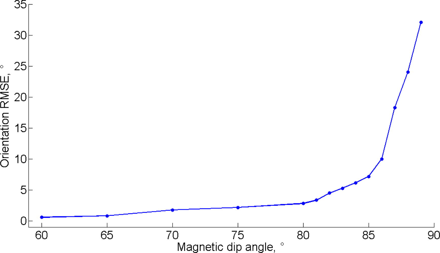
The salient steps of the observability proof are reported in Appendix A, where the matrices X1, X2, X3, and hence the matrix D, do not need to be computed explicitly. In short, the system of Equation (22) is certainly locally weakly observable when: (a) the magnetic field has components in the horizontal plane, which is necessary to have the horizontal reference for heading estimation; (b) at least one degree of rotational freedom is excited. Remind that the magnetic dip angle, also called magnetic inclination, is the angle the Earth’s magnetic field makes with the surface of the Earth; the observability condition (a) fails when the dip angle is ±90° (e.g., close to the Poles). Running the estimation algorithm during periods when the observability is not guaranteed—when the magnetic dip angle is close to ±90° or the IMU is in quasi-static conditions—is likely to degrade seriously the state estimation accuracy. This fact has to be verified by assessing the system’s behavior by computer simulations and experimental testing.
3.5. Filter Assessment
The performance metrics are based on computing the error quaternion , where q̄t and q̄ are the true and the estimated quaternion, respectively. In the present context the term true implies the use of synthetic or experimental motion data to carry out the test procedure. An obvious advantage of working with synthetic signals is that the errors incurred in estimating the state vector components can be compared with the bounds that are predicted by the error covariance matrix produced by the EKF. This is a useful feature to assess the filter convergence and to diagnose a number of potential problems arising in its numerical implementation. Experimental motion data can be captured, e.g., from an optoelectronic motion tracker, so as to define the ground truth reference for filter assessment.
The error quaternion represents the rotation that brings the estimated body frame onto the true body frame. Its scalar component can be used to derive the orientation error Δθ, according to the equation Δθ = 2arccos(Δq4) The performance metrics are expressed in terms of the root-mean-square-value of the orientation error (RMSEq), averaged over the number of either the Monte Carlo simulation runs or the experimental trials available. Alternatively, a set of estimated and reference Euler angles (roll, pitch, yaw or heading) can be computed from q̄t and q̄ using standard conversion formulas, and the filter performance can be summarized by presenting the RMSEs of the Euler angles, again averaged over the number of either the Monte Carlo simulation runs or the experimental trials available. Although the calculations for orientation are not performed using Euler angles, the results can be presented in this way for better interpretation.
3.6. Computer Simulations
The body-fixed frame has a fixed origin, and it is aligned with the Earth-fixed frame at the initial time of each simulation trial. Our choice of the earth-fixed frame follows the North-East-Down (NED) convention: the gravity vector is g = [0 0 g]T (g = 9.81 m/s2), and the earth magnetic field is h = [hx 0 hz]T (hx = 0.26 Gauss; hz = 0.37 Gauss). The simulated field strength is approximately 0.45 Gauss, with a magnetic dip angle δ ≈ 55°, situations typical of our latitudes. A magnetically perturbed environment is simulated by adding h with the output of a routine that generates samples from a Gauss-Markov vector random process with statistically independent components.
The angular velocity time functions are given as input to the simulation program. The true quaternion time functions are obtained by time integrating the kinematic Equation (9) at the sampling frequency of fs = 4 kHz, which is high enough to make integration errors negligible; the quaternion time functions are then time-decimated down to fs = 100 Hz (the sampling frequency used in many popular orientation trackers). Two distinct conditions are tested: static conditions, in which case the angular velocity is null, and then the IMU does not change the initial orientation; dynamic conditions, i.e., following an initial period of rest, a pure sinusoidal rotation around the vertical axis is simulated (amplitude: 100°/s; frequency: 1 Hz). In either case simulation trials last 10 min.
The magnetic field and the gravity vector can be expressed in the body-frame using the computed quaternions. White Gaussian noise is then injected into the body-referenced sensor time functions to simulate the effect of specified amounts of measurement noise: σa = 1 − 5 mg; σh = 1 mGauss. In dynamic conditions the value of σa is chosen relatively high as compared with values measured during on-bench calibration tests of MEMS accelerometers, which are less than 1 mg; this is to account for the minute motions that affect on-body IMUs, even when the body is quasi-static. No scale factor or bias errors are considered for the IMU sensors, with the exception of the gyro: the gyro time functions are corrupted by addition of a Gaussian white measurement noise component with standard deviation σg = 0.4°/s and a fixed offset (e.g., bg = [1 − 0.5 0.75]T °/s).
The different treatment of IMU sensors is motivated by the weight an uncompensated gyro bias has on the error budget of an inertial orientation sensor and consequently by our desire to always enable the compensation of gyro bias in our filter. The following two EKF implementations are considered: EKF-MA and EKF-MB, which differ in enabling the compensation of magnetic disturbances or not; in order to disable the compensation of magnetic disturbances, bσh = 0 and α = 0 are plugged in Equation (27). The two methods are tested in static and dynamic conditions, when either the magnetic variation is markovian, namely it follows the Gauss-Markov model of Equation (20) (magnetically perturbed environment, MPE), or when the magnetic variation is null (magnetically clean environment, MCE). For each combination of method and condition, N = 10 Monte Carlo runs are performed, and the values of orientation RMSEq are reported (mean ± standard deviation, SD). Another set of simulations is carried for different values of the magnetic inclination, from 55° to 90° (dynamic conditions—method MA). The aim is to verify the filter behavior in difficult observability conditions. The filter parameter setting is given in Table 1.
3.7. Experimental Validation
The MTx orientation tracker by Xsens Technologies B.V. (Enschede, The Netherlands) is used for carrying out the experimental validation. The raw sensor data are delivered through a USB interface to the host computer at a rate of 100 Hz, together with the Euler angle time functions estimated by the proprietary EKF, henceforth called the Xsens-EKF. The IMU sensors are calibrated before starting the experimental session as described in [26,27]; by contrast, no bias capture is considered for the gyro. The initial orientation of the sensor frame relative to the marker frame is found by taking data during the rest period when the IMU is still.
The tests for validation in static and dynamic conditions are carried out within one of our lab rooms. The static test, whose duration is 10 min, consists of leaving the IMU still on a table that is placed far from current wires, computer appliances, and ferromagnetic materials. A magnetic disturbance is induced at the time when a cell phone is placed close to the IMU; the cell phone is left in place for a while, then it is removed, so as to recover the initial magnetic field. The test for validation in dynamic conditions is performed as follows. The IMU is fastened to a 50 cm 50 cm wooden plate using double-side adhesive tape. The plate is raised by hand slightly over the table and then it is freely moved around; toward the end of the trial, which lasts about 137 s, the plate is replaced approximately in the same pose. The working volume visited by the plate during the motion trial is 100 cm × 50 cm × 60 cm. The plate orientation is recorded using a six-camera Vicon optical motion capturing system with a sampling rate of fs = 100 Hz. The IMU and Vicon data streams are electronically time-synchronized. The Vicon system measures the position of four reflective markers (diameter: 14 mm) arranged at the corners of the plate to form a square with side 45 cm. The accuracy of the marker frame is determined by analyzing the relative motion of two markers: the RMS of the Vicon orientation error Δθ is assumed in the same order as the RMS distance variation divided by the distance between two markers (Δθ < 0.5°). The RMSEs of the Euler angles and the RMSEq of the orientation are presented using the Euler angles time functions computed by the Vicon system as the truth reference. The filter parameter setting we choose for the experimental validation is reported in Table 2. The orientation sensor delivers the data from the magnetic sensor in arbitrary units.
4. Results
4.1. Computer Simulations
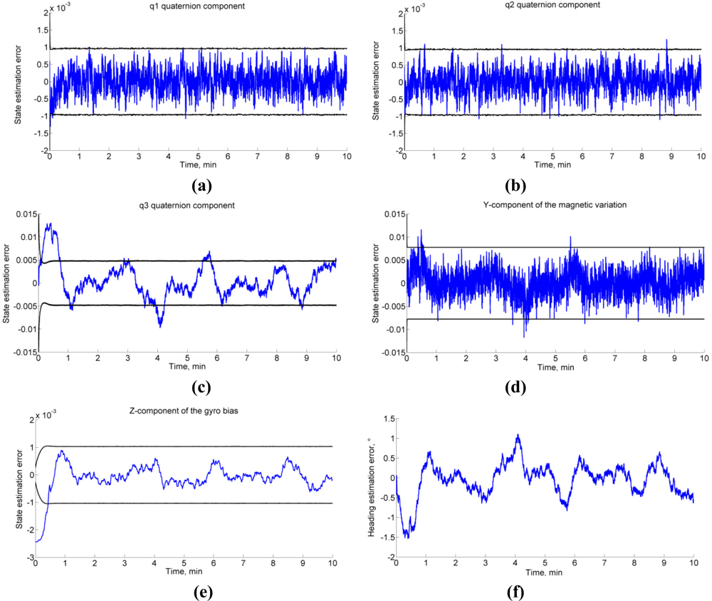
The Monte Carlo results are reported in Table 3. The EKF-MA performs better than the EKF-MB in a magnetically markovian environment, according to a paired-sample t-test (statistically significant difference, SSD at p < 0.001 and p < 0.01, in dynamic and static conditions). In the case of null magnetic variations, the EKF-MA performs as the EKF-MB. Figure 1 depicts the typical behavior in dynamic conditions. As for the second condition of observability, the EKF-MA is tested in the same conditions leading to the data in Figure 1, for different values of the magnetic dip angle, Figure 2.
4.2. Experimental Validation: Static Test
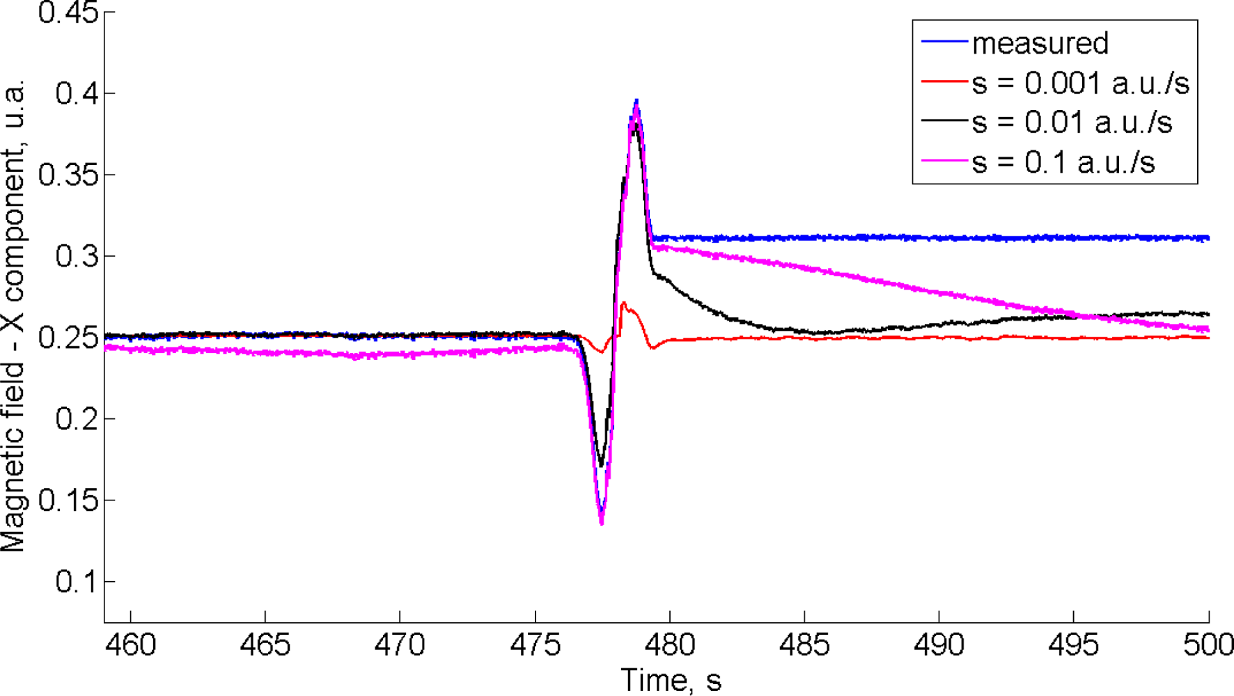
In Figure 3 we plot, in blue, the component of the magnetic field along the X-direction (earth-fixed frame), as is measured by the magnetic sensor. Since the test environment is almost magnetically unperturbed before placing the cell phone nearby the IMU at time t1 = 476 s, the measured magnetic field is the true magnetic field existing in the room with very good approximation. The EKF-MA is tested using three different values of the process noise standard deviation bσh.
All the other parameters being the same as in Table 2, these values are: bσh = 0.001 a.u./s (red); bσh = 0.01 a.u./s (black); bσh = 0.1 a.u./s (magenta). The RMS value of the difference between estimated and measured X-components of the magnetic field up to time t1 increases from 15 × 10−5 a.u. (bσh = 0.001 a.u./s) to 8.4 × 10⁻³ a.u. (bσh = 0.1 a.u./s). The magnetic disturbance from t1 to when the cell phone comes to a stop at time t2 = 480 s is best tracked with higher values of bσh. However, when the magnetic field is not time variant anymore from time t2 on, the filter behavior is unsatisfactory. The estimated heading angle is reported in Figure 4.
4.3. Experimental Validation: Dynamic Test
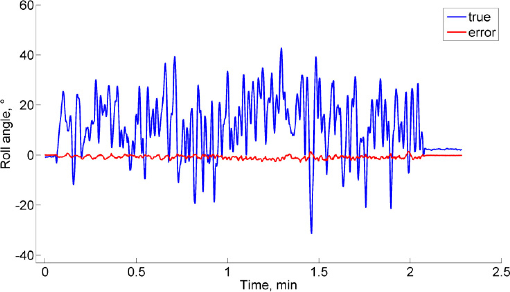
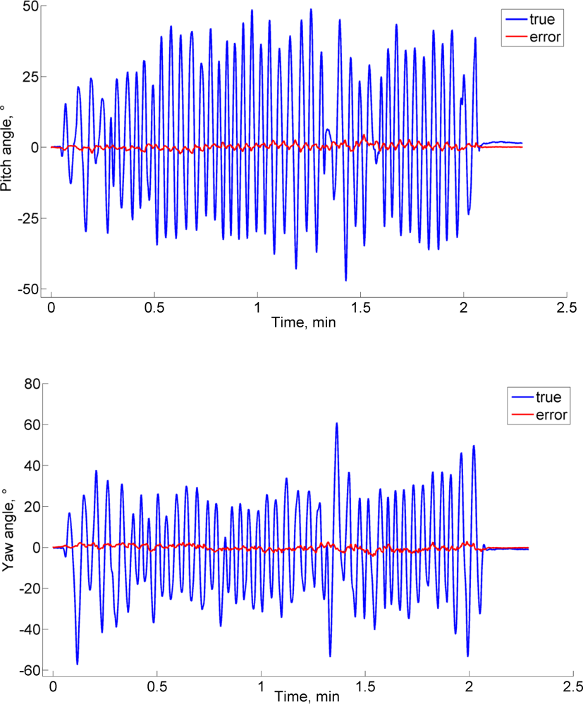
The norm of the acceleration magnitude is 1 g ± 60 mg throughout the trial, and the coefficient of variation of the norm of the measured magnetic field is about 1%. The RMSE of the Euler angles are reported in Table 4 for the EKF-MA and the EKF-MB. As a matter of comparison, we also report the errors statistics in three other cases: (a) when only the gyro angular velocities are used and the aiding sensors are disabled; (b) when only the accelerometer and magnetic sensor data are involved in determining the orientation using the TRIAD method; (c) when the orientation is estimated by the Xsens-EKF. The Euler angle time functions estimated by the Vicon system are reported with superimposed the errors incurred by the EKF-MA in Figure 5.
4. Discussion and Concluding Remarks
The conditions for the observability of the KF-based algorithm for IMU orientation tracking are based on the rank-condition of the observability matrix Equation (39). These conditions require that the local magnetic field, which may include magnetic variations superimposed to the earth magnetic field, and the gravity vector are not collinear; moreover, at least one rotational degree of freedom would excite the system. The computer simulations clearly show the relevance of the first condition. Indeed, when the magnetic dip angle becomes too large, the heading estimation accuracy undergoes an impressive degradation. Conversely, the computer simulations, and experimental testing as well, demonstrate that the condition concerning the IMU motion is not critical. In static conditions, the filter is stable and its performances are similar to those achieved in dynamic conditions. In general, we observe some problems of filter consistency. In particular, difficulties exist in picking up the third component of the quaternion and the horizontal magnetic states, as shown in Figure 1(c–d). The errors in these estimated state vector components turn out to be highly correlated in time, which is not reflected in the expression of the computed error state covariance matrix; moreover, while the compensation of gyro bias is generally fast, some possible problems exist for its Z-component, Figure 1(e). These behaviors are not unexpected: the estimated values of heading, horizontal component of the acting magnetic field and gyro bias component in the vertical direction must necessarily interact in the attempt to explain the information available to the filter. In other words, the observability conditions can never be too good. However, a safe start in a magnetic homogeneous area [7], and standing still few seconds to carry out the IMU alignment [8] are useful expedients to ensure the validity of the linear approximation of the IMU orientation tracking process. Some disadvantages of the linearization procedure implemented in an EKF are indeed sensitivity to initial conditions, biases in the estimation errors, and critical problems of convergence and filter stability, especially when the sampling interval is too large [28].
The results of the experimental validation support the results of the Monte Carlo study, either in the static case or in dynamic conditions. The importance of implementing sensor fusion algorithms is stressed by the results offered in Table 5. Presently, the reason why the yaw estimates from the Xsens-EKF start to diverge after about 40 s is unknown. The advantage of the compensation of the magnetic disturbances is shown in a situation where the level of contamination is low. It should be noted the importance of providing the filter with some sort of adaptability to the magnetic environment. In this regard, the results of the validation test in static conditions gives rise to several interesting considerations. Since the magnetic variations are quite small, the mechanism of magnetic disturbance compensation is on, with a small value of the process noise standard deviation. This helps making the filter stable; however, its capability of dealing with the magnetic disturbance, when it occurs, is very limited. If, in the effort to deal with the magnetic disturbance, we increase the process noise, the ability to follow the magnetic variations when they occur is remarkable, however the filter may lose track when the magnetic variations are small. On one hand, the injection of process noise is known as a useful recipe to account for mismodeling problems, and even to make the filter response faster [30]; on the other hand, excess process noise is also responsible for less accurate state estimates in benign tracking conditions.
The importance of implementing sensor fusion algorithms is further outlined by the results reported in Table 4. Two further implementations are considered: “only gyro” refers to the case when the EKF is unaided by the accelerometer and the magnetic sensor, and the orientation information is obtained exclusively by time-integrating noisy gyro signals from initial conditions we assume, for simplicity, to be known at the same level of accuracy as in EKF-MA and EKF-MB (we ignore the details of the Xsens’ initialization procedure). This can be obtained by plugging high values of the accelerometer and magnetic sensor measurement noise standard deviation into the filter matrix R. On the contrary, the column named “gyro-free” in Table 4 refers to the case when a gyro-free measurement unit is considered. In this case, only the accelerometer and the magnetic sensor are used: their information is combined while solving a specific instance of the Wahba’s problem using the TRIAD algorithm, which is often used to combine measured gravity and Earth magnetic field vectors, for slow motions occurring in magnetically clean environments. Either for the “only gyro” or the “gyro-free” systems, it is worth noting that the stabilization of inclination (roll and pitch) and heading (yaw) is achieved just to a limited extent. In the “only gyro” system, the limited stabilization is a consequence of the random-walk integration of wideband gyro measurement noise, while, in the “gyro-free” system, it is a consequence of the fact that, being a single-frame algorithm for orientation determination, the TRIAD per se does not smooth the estimates it produces: even small tremulous movements affecting the accelerometer and any magnetic disturbance in the environment combine their effects to produce noisy orientation estimates. Although the “only gyro” system seems to be almost equivalent to the “gyro-free” system in this particular experimental trial, it must be remembered that random-walk errors tend to grow unbounded over time, while the high-frequency noise affecting the “gyro-free” system is virtually drift-free. However, the “gyro-free” system is completely blind and vulnerable to abrupt changes in the body motion and to magnetic variations in the environment. On the other hand, the EKF is capable of making the best use of the available information, and provides outstanding performance as compared with the “only gyro” and the “gyro-free” systems. Although having a limited ability to overcome magnetic variations, as shown in the static test results, the EKF we have developed may be protected against the effects of body motion using vector selection schemes such as those implemented in [2], which make it adaptive to some extent (R-adaptation, or adaptation of the measurement noise covariance matrix R is involved in [2]). These schemes are not considered here. An interesting avenue of research will concern how to make the EKF Q-adaptive, namely how the process noise covariance matrix Q may be changed at run-time to reflect varying magnetic conditions. These considerations stress the importance of developing adaptive EKFs: this is beyond the scope of this paper and it is the subject of our current research. At the present time, we are investigating the rank-condition of observability matrices built from gradients of the Lie derivatives in our research on adaptive EKFs that aims at the compensation of magnetic disturbances in strongly perturbed environments.
The main contribution of this paper concerns the presentation of a method for testing the observability of KFs applied to a problem of orientation determination using inertial/magnetic sensors. Oftentimes, KFs are developed exploiting the considerable freedom in choosing the state and measurement equations, without paying proper consideration to possible problems of observability. This is the first time the observability rank criterion based on Lie derivatives is applied to test the observability of a quaternion-based EKF that is developed for determining the orientation of a rigid body using inertial/magnetic sensors. The formal demonstration of the conditions of observability and, in addition to that, the results of a set of Monte Carlo computer simulations and few experimental trials are offered in support of our approach.
Acknowledgments
This work has been supported by funds from the Italian Ministry of University and Research. The author is indebted to Andrea Mannini for his assistance in performing the experiments.
References
- Welch, GF; Foxlin, E. Motion tracking: No silver bullet, but a respectable arsenal. IEEE Comput. Graph. Appl 2002, 22, 24–38. [Google Scholar]
- Sabatini, AM. Quaternion-based extended Kalman filter for determining orientation by inertial and magnetic sensing. IEEE Trans. Biomed. Eng 2006, 53, 1346–1356. [Google Scholar]
- Yun, X; Bachmann, ER; McGhee, RB. A simplified quaternion-based algorithm for orientation estimation from earth gravity and magnetic field measurements. IEEE Trans. Instrum. Meas 2008, 57, 638–650. [Google Scholar]
- Lee, JK; Park, EJ. A fast quaternion-based orientation optimizer via virtual rotation for human motion tracking. IEEE Trans. Biomed. Eng 2009, 56, 1574–1582. [Google Scholar]
- Veltink, PH; Bussmann, HBJ; de Vries, WHK; Martens, WLJ; Van Lummel, RC. Detection of static and dynamic activities using uniaxial accelerometers. IEEE Trans. Rehabil. Eng 1996, 4, 375–385. [Google Scholar]
- Bachmann, ER; Yun, X; Peterson, CW. An investigation of the effects of magnetic variations on inertial/magnetic orientation sensors. Proceedings of IEEE International Conference on Robotics and Automation (ICRA '04), New Orleans, LA, USA, 26 April–1 May 2004; pp. 1115–1122.
- de Vries, WHK; Veeger, HEJ; Baten, CTM; van der Helm, FCT. Magnetic distortion in motion labs, implications for validating inertial magnetic sensors. Gait Posture 2009, 29, 535–541. [Google Scholar]
- Sabatini, AM. Estimating three-dimensional orientation of human body parts by inertial/magnetic sensing. Sensors 2011, 11, 1489–1525. [Google Scholar]
- Gallagher, A; Matsuoka, Y; Wei-Tech, A. An efficient real-time human posture tracking algorithm using low-cost inertial and magnetic sensors. Proceedings of IEEE/RSJ International Conference on Intelligent Robots and Systems (IROS 2004), Sendai, Japan, 28 September–2 October 2004; pp. 2967–2972.
- Wahba, G. A least-square estimate of spacecraft attitude. SIAM Rev 1965, 7, 409. [Google Scholar]
- Gebre-Egziabher, D; Elkaim, GH; Powell, JD; Parkinson, BW. A gyro-free quaternion-based attitude determination system suitable for implementation using low cost sensors. Proceedings of IEEE Position Location and Navigation Symposium (PLANS '00), San Diego, CA, USA, 13–16 March 2000; pp. 185–192.
- Markley, FL. Attitude determination and parameter estimation using vector observations: Theory. J. Astronaut. Sci 1989, 37, 41–58. [Google Scholar]
- Welch, GF. The use of the Kalman filter for human motion tracking in virtual reality. Presence 2009, 18, 72–91. [Google Scholar]
- Brown, RG; Hwang, PYC. Introduction to Random Signals and Applied Kalman Filtering; John Wiley & Sons: New York, NY, USA, 1997. [Google Scholar]
- Foxlin, E. Inertial head-tracker sensor fusion by a complementary separate-bias Kalman filter. Proceedings of IEEE Virtual Reality Annual International Symposium, Santa Clara, CA, USA, 30 March–3 April 1996; pp. 185–194.
- Luinge, HJ; Veltink, PH. Inclination measurement of human movement using a 3-D accelerometer with autocalibration. IEEE Trans. Neur. Syst. Rehabil. Eng 2004, 12, 112–121. [Google Scholar]
- Roetenberg, D; Luinge, HJ; Baten, CTM; Veltink, PH. Compensation of magnetic disturbances improves inertial and magnetic sensing of human body segment orientation. IEEE Trans. Neur. Syst. Rehabil. Eng 2005, 13, 395–405. [Google Scholar]
- Yun, X; Bachmann, ER. Design, implementation, and experimental results of a quaternion-based Kalman filter for human body motion tracking. IEEE Trans. Robot 2006, 22, 1216–1227. [Google Scholar]
- Lefferts, EJ; Markley, FL; Shuster, MD. Kalman filtering for spacecraft attitude estimation. J. Guid 1982, 5, 417–429. [Google Scholar]
- Harada, T; Mori, T; Sato, T. Development of a tiny orientation estimation device to operate under motion and magnetic disturbance. Int. J. Rob. Res 2007, 26, 547–559. [Google Scholar]
- Tomé, P; Yalak, O. Improvement of orientation estimation in pedestrian navigation by compensation of magnetic disturbances. J. Navig 2008, 55, 179–190. [Google Scholar]
- Foxlin, E; Harrington, M; Altshuler, Y. Miniature 6-DOF inertial system for tracking HMDs. SPIE Proc 1998, 3362, 214–228. [Google Scholar]
- Mirzaei, FM; Roumeliotis, SI. A Kalman-filter-based algorithm for IMU-camera calibration: Observability analysis and performance evaluation. IEEE Trans. Robot 2008, 24, 1143–1156. [Google Scholar]
- Shuster, MD. A survey of attitude representations. J. Astronaut. Sci 1993, 41, 439–517. [Google Scholar]
- Isidori, A. Nonlinear Control Systems; Springer Verlag: London, UK, 1995. [Google Scholar]
- Ferraris, F; Grimaldi, U; Parvis, M. Procedure for effortless in-field calibration of three-axis rate gyros and accelerometers. Sens. Mater 1995, 7, 311–330. [Google Scholar]
- Gebre-Egziabher, D; Elkaim, GH; Powell, JD; Parkinson, BW. A non-linear, two-step estimation algorithm for calibrating solid-state strapdown magnetometers. Proceedings of 8th International Conference on Navigation Systems, St Petersburg, Russia, 28–30 May 2001.
- Crassidis, JL; Markley, FL. Unscented filtering for spacecraft attitude estimation. J. Guid. Contr. Dynam 2003, 26, 536–542. [Google Scholar]
- Sabatini, AM. Quaternion-based strap-down integration method for applications of inertial sensing to gait analysis. Med. Biol. Eng. Comput 2005, 43, 94–101. [Google Scholar]
- Maybeck, PS. Stochastic Models, Estimation and Control; Academic Press: New York, NY, USA, 1982. [Google Scholar]
- Markley, FL. Attitude error representations for Kalman filtering. J. Guid. Contr. Dynam 2003, 26, 311–317. [Google Scholar]
- Choukroun, D; Bar-Itzhack, IY; Oshman, Y. Novel quaternion Kalman filter. IEEE Trans. Aerosp. Electron. Syst 2006, 41, 174–190. [Google Scholar]
- Shuster, MD; Oh, S. Three-axis attitude determination from vector observations. J. Guid. Contr 1981, 4, 70–77. [Google Scholar]
Appendix
We prove the conditions under which the 6 × 3 matrix A is full rank:
Next, we prove the rank conditions for the 10 × 7 matrix B, for which we have:
By performing Gaussian elimination on the corresponding rows of O and eliminating all the elements of the involved columns we obtain:
Since a valid DCM is non-singular, we conclude that the observability matrix is full rank when: (a) the magnetic field and the gravity vectors are not collinear; (b) at least one degree of rotational freedom is excited.


| MPE-MA | MCE-MA | MPE-MB | MCE-MB | |
|---|---|---|---|---|
| σg, °/s | 0.4 | 0.4 | 0.4 | 0.4 |
| bσg, °/s2 | 0.01 | 0.01 | 0.01 | 0.01 |
| bσh, mGauss/s | 10 | 1 | 0 | 0 |
| α, s−1 | 1 | 1 | 0 | 0 |
| σa, mg | 5 | 5 | 5 | 5 |
| σh, mGauss | 1 | 1 | 1 | 1 |
| Static | Dynamic | |
|---|---|---|
| σg, °/s | 0.4 | 0.4 |
| bσg, °/s2 | 0.01 | 0.01 |
| bσh, u.a./s (×10−3) | 10 | 10 |
| α, s−1 | 10 | 10 |
| σa, mg | 1 | 5 |
| σh, mGauss | 1 | 1 |
| Condition: MPE | |
| EKF-MA | |
| Static test | 0.93 ± 0.24 *** |
| Dynamic | 1.05 ± 0.24 ** |
| EKF-MB | |
| Static test | 1.27 ± 0.18 *** |
| Dynamic | 1.53 ± 0.21 ** |
| Condition: MCE | |
| EKF-MA | |
| Static test | 0.29 ± 0.11 |
| Dynamic | 0.32 ± 0.08 |
| EKF-MB | |
| Static test | 0.22 ± 0.11 |
| Dynamic | 0.24 ± 0.15 |
**SSD at p < 0.01;***SSD at p < 0.001.
| EKF-MA | EKF-MB | Only gyro | TRIAD | Xsens-EKF | |
|---|---|---|---|---|---|
| Roll, ° | 0.89 | 1.02 | 2.14 | 2.15 | 0.92 |
| Pitch, ° | 0.97 | 0.93 | 3.85 | 4.49 | 0.71 |
| Yaw, ° | 1.14 | 1.18 | 7.62 | 5.81 | 10.48 |
| Orientation,° | 1.63 | 1.69 | 8.68 | 7.44 | 10.60 |
© 2011 by the authors; licensee MDPI, Basel, Switzerland. This article is an open access article distributed under the terms and conditions of the Creative Commons Attribution license (http://creativecommons.org/licenses/by/3.0/).
Share and Cite
Sabatini, A.M. Kalman-Filter-Based Orientation Determination Using Inertial/Magnetic Sensors: Observability Analysis and Performance Evaluation. Sensors 2011, 11, 9182-9206. https://doi.org/10.3390/s111009182
Sabatini AM. Kalman-Filter-Based Orientation Determination Using Inertial/Magnetic Sensors: Observability Analysis and Performance Evaluation. Sensors. 2011; 11(10):9182-9206. https://doi.org/10.3390/s111009182
Chicago/Turabian StyleSabatini, Angelo Maria. 2011. "Kalman-Filter-Based Orientation Determination Using Inertial/Magnetic Sensors: Observability Analysis and Performance Evaluation" Sensors 11, no. 10: 9182-9206. https://doi.org/10.3390/s111009182