Over recent years, fault diagnosis for networked control system (NCS) using the mode-based analytical redundancy method have received significant attention. In [1,2], the overviews of main ideas and results on fault diagnosis of NCS are given, including the fundamentals of fault diagnosis for NCS with information scheduling, fault diagnosis approaches based on the simplified time-delayed system models and the quasi T-S fuzzy model, and fault diagnosis for linear and nonlinear NCS with long time-delay. However, most of the available results make use of time-triggered state estimation techniques by sampling the output of plant at an essentially equidistant time instant. Because the sampling period is determined according to the worst case operation conditions that rarely occur, the time-triggered sampling leads to a conservative usage of the communication bandwidth.

On the other hand, recent advances in computing and communication technologies enable the wireless networks (e.g., Bluetooth, wirelessHART and ZigBee) to rapidly replace wired networks in many applications, including industrial control and monitoring, home automation and consumer electronics, security and military sensing, and health monitoring [3,4]. Though the wireless channels are easier and cheaper to deploy and avoid cumbersome cabling, they also pose serious resource constraints. Therefore, applying the time-triggered sampling method to the wireless NCS may have some negative effects on the estimation and control performance of system, such as wasting the scarce communication resource and further shortening the lifetime of overall system. Since the event-triggered sampling strategies present a number of potential advantages for NCS, such as clock-free operation, less traffic requirement, and better resource utilization, they have been regarded as the possible and important alternatives to the time-triggered sampling.

Until now, numerous event-triggered sampling concepts have been proposed in the literature, such as send-on-delta sampling [5,6], level-crossing sampling [7], deadband sampling [8], Lebesgue sampling [9], send-on-area sampling [10], error energy sampling [11], self-triggered sampling [12], etc. Although these schemes have different terminologies, the same attribute is that the signal is sampled only when an a priori defined events occurs in the data monitored by sensors. For instance, the studies in [5–9] are concerned with the same sampling criterion where the event is defined as that the difference Δ between the current sensor value and the last transmitted one is greater than a given threshold. While in [10] and [11], the event is that the integral and energy of Δ is greater than a given threshold, respectively. Because of inherent distinctive benefits, the so-called event-triggered state estimation and event-based control for NCS with event-triggered sampling schemes have gained increasing attention. In this paper, however, we focus our attention on the event-triggered state estimation for the purpose of fault diagnosis. In relation to a parallel line of research on the event-based control, we refer the readers to the literature, e.g., [12,13].

In the context of state estimation, although the time-triggered state estimation over networks with network-induced effects taken into account have made great progress (see, e.g., [14–17]), research on the event-triggered state estimation is relatively lacking apart from several works [6,10,18–26]. It is well known that utilizing more sensors can potentially improve the performance of the estimation algorithms. However, using too many sensors can in turn create bottlenecks in the communication resource when these sensors compete for bandwidth. As a result, the studies in [18–21] explore the tradeoff between communication and estimation performance. Rather than sending every raw measurement to the remote estimator via network, a so-called controlled communication policy was adapted, which firstly obtain the local estimate x̃_k|k from the raw sensor measurements and then compare x̃_k|k with the remote estimate to decide whether or not it is worth sending data x̃_k|k. Also, Reference [21] proposes an optimal communication policy by dynamic programming and value iteration to minimize a long-term average cost function, which is related to the difference between the local and remote estimate. Based on the send-on-delta method, Reference [6] proposes a modified Kalman filter where computed output with increased measurement noise covariance is used when there is no sensor data transmission. The authors also discuss how to choose the threshold which is a trade-off parameter between the sensor data transmission rate and the estimation performance. Reference [22] extends the previous work [6] to address how to determine the measurement value at a sensor node if it does not send data. To avoid the inability of send-on-delta method in detecting the signal oscillations or steady-state error, Reference [10] proposes a novel scheme called send-on-area and then formulates a networked estimator based on Kalman filter to estimate the states of the system. More recently, Reference [23] proposes a networked estimator for event-triggered sampling systems with packet dropouts. Reference [24] develops an event-triggered estimator which is updated both when an event occurs with a received measurement sample, as well as at sampling instants synchronous in time without receiving a measurement sample. However, to the authors’ knowledge, fault diagnosis of networked control systems making use of the event-triggered state estimation method has not been addressed, which motivates the current study of this paper.

In this paper, we show our attention on the implementation problem of a modified fault isolation filter (FIF) for NCS with event-triggered sampling and multiple faults. By the send-on-delta scheme which is one of the event-triggered sampling strategies, it means that the sensor data is transmitted only when the absolute value of difference between the current sensor value and the previously transmitted one is greater than the given threshold value. Based on this scheme, a modified FIF for a discrete-time NCS with multiple faults is then implemented by a particular form of the Kalman filter. The rest of this paper is organized as follows. The modelling of NCS with event-triggered sampling scheme is presented in Section 2. A modified FIF is proposed in Section 3. An illustrative example is presented in Section 4 to show the effectiveness of the result. The paper is concluded in Section 5.

Notations: In what follows, if not explicitly stated, matrices are assumed to have compatible dimensions. Z₊ denotes the set of nonnegative integer numbers. ℛⁿ and ℛ^n×m are, respectively, the n-dimensional Euclidean space and the set of n × m real matrices. A^T denotes the transpose matrix or vector A. A⁻¹ and A⁺ represent the inverse and pseudo-inverse of A, respectively. diag(a₁,…,a_n) refers to an n × n diagonal matrix with a_i as its ith diagonal entry. rank(A) stands for the rank operator of matrix A. ℰ(x) represents the mathematical expectation of random variable x. x ∼ 𝒩(μ, Σ) means that the random vector satisfies the normal distribution with mean value μ and covariance matrix Σ. 𝒫(x|y) means the conditional probability distribution of x given y. Sign function is defined as sign ( x ) = { 1 , x ≥ 0 ; − 1 , x < 0.

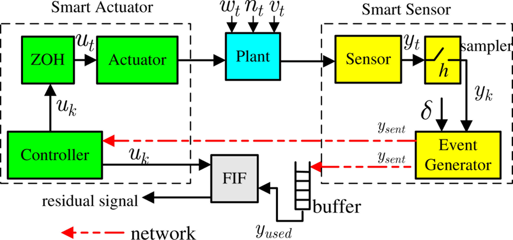
The architecture of NCS with event-sampling discussed in this paper is shown in Figure 1, where the closed-loop system consists of a plant with smart sensors and actuators, a remote FIF and a wireless network channel. The controller, FIF and actuator are assumed to be logically integrated. Thus, control commands do not need to experience any wireless transmission. This configuration represents a system, e.g., wireless sensor/actuator system, where actuation is inexpensive but sensor measurements are transmitted to the controller or FIF by sensors with a limited energy.

Since the event generator, the controller and the FIF have to be implemented on smart sensors and actuators by means of digital hardware, a discrete-time plant model is considered as the alterative to the continuous plant together with a zero-order hold and a sampler. The state evolution and sensor measurement equation are given as follows, respectively: (1) { x k + 1 = Ax k + Bu k + Fn k + w k         y k = Cx k + v kwhere x_k ∈ ℛⁿ is the state vector, u_k is the known manipulated input, F = [ f 1 f 2 … f q ] ∈ ℛ n × q is the fault distribution matrix, n_k ∈ ℛ^q is the fault vector, and y k = [ y k 1 … y k i … y k m ] T ∈ ℛ m the output observation vector of sensors. We assume that the initial state vector x₀, process noise w_k and measurement noise v_k are uncorrelated, zero mean white Gaussian random processes with x₀ ˜ 𝒩 (μ₀, Σ₀), w_k ˜ 𝒩(0, W) v_k ˜ 𝒩(0, R), where Σ₀, W and R are symmetric, positive definite matrices.

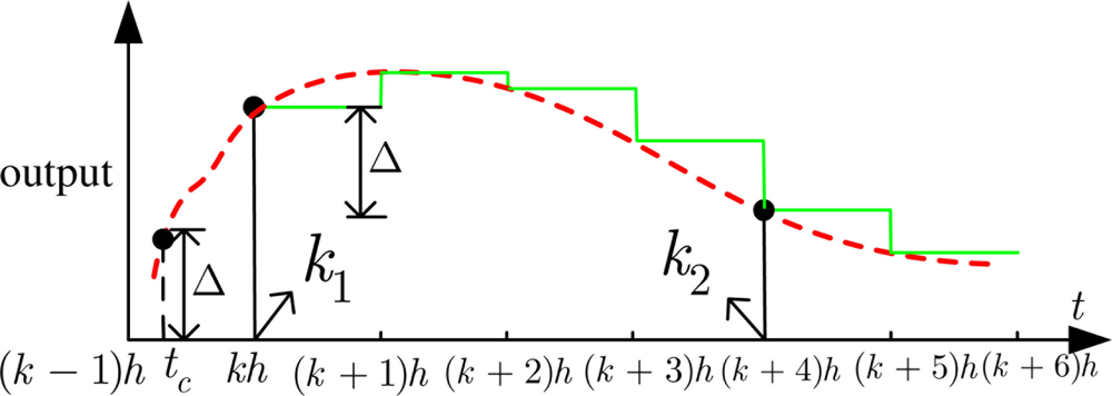
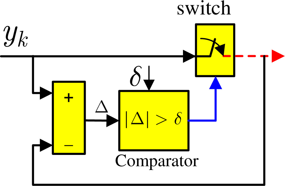
As shown in Figure 1, the smart sensor numbered i has a sampler which regularly samples the sensor measurement with period h and an event generator to decide whether or not to send new sensor measurement through the network. The event generator therein, also known as send-on-delta scheme, is illustrated in Figure 2 where the sensor data y k i is transmitted only when the absolute value of difference between the current sensor value y k i and the previously transmitted one y sent i is greater than the given threshold value δ_i, namely (2) | y k i − y sent i | > δ iwhere δ_i is simply determined according to x-fold of the maximal amplitude of y k i.

Obviously, all the transmitted measurements y sent i are the event-triggered samplers which are subsequences of the raw measurement y k i. For instance, if the time instant when the previous event occurs is denoted as k_j ∈ Z₊, the event-triggered sampling condition (2) is further formulated as (3) | y k i − y k j i | > δ i , k ∈ [ k j , k j + 1 ) , k j ∈ Z +

However, the time instant k_j (j = 1, 2....) can not be precisely determined because of the sampler, which is significantly different from the continuous one introduced in e.g., [5,6]. As shown in Figure 3, the dash line and real line represent the sensor measurement in the continuous time and discrete time, respectively. In the continuous time case, the time t_c when an event occurs can be exactly known since the measurement of plant is continuously updated by the sensor. While in the discrete time, the events have to be generated at the subsequent discrete time steps, e.g., k₁ equivalent to kh, k₂ equivalent to (k + 4)h, since the measurement is only updated at some discrete time instants and remains constant in the inter-sampling interval. Although producing the unsent measurements, e.g., the sample at the time instant (k + 1)h, wastes a bit of computing resource, the unsent measurements in turn save a lot of communication resources. In a sense of improving the resource utilization, applying the event-triggered sampling schemes to discrete-time plant is also meaningful. The reason is that wireless communication consumes more energy than information processing. As noted in [5], a sensor node can execute 3,000 instructions for the same energy cost of sending a single bit at the distance of 100 meters by radio.

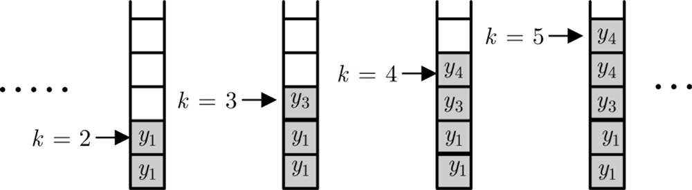
In the sequel, we further assume that all sensor measurements are time-stamped and the network is communication link without packet losses and time delays. For the purpose of reducing communication, only parts of the raw measurements will be communicated to the remote FIF by the send-on-delta scheme. Through the communication link, all the event-triggered samplers { y k j i } j = 1 ∞ are then stored in an infinite buffer. If sensor measurement y k i does not yet arrive at the buffer at time instant k, it means that the current value y k i has not significantly changed in contrast to the previous event-triggered sampler y k j i. In this case, the previous buffer value z k − 1 i whose value is equivalent to y k j i will be stored in the k-slot of the buffer, as illustrated in Figure 4.

Furthermore, the arrival of the measurement y k i at time k is defined as a binary variable θ k i, namely θ k i = 1 when y k i arrives at the buffer at time instant k, otherwise θ k i = 0. Rather than considering the design problem where only the probabilities of θ k i at each time instant is known and the research interest lies in studying the effect of loss and delay probabilities, we address the implementation problem where the value of θ k i at each time instant is known in advance. The last received value of i-th sensor output at time instant k_j is denoted as y k j i. If there is no sensor data received for k > k_j, the estimator node considers that the measurement value of the i-th sensor output y k i is still equal to y k j i, but the measurement noise is increased from υ k i to υ ¯ k i = υ k i + Δ k , k j i where Δ k , k j i = y k j i − y k i satisfies | Δ k , k j i | ≤ δ i.

From the existing literature [6,22], the assumption that Δ k , k j i has a uniform distribution with zero mean and a variance δ i 2 / 3 is valid only if the measurement covariance R > δ². Otherwise, the mean and variance of Δ_i(k, k_j) is sign ( y k j i − y k j − 1 i ) * δ i / 2 and δ_i/12 respectively. Thus, the measurements z k i which the FIF will use for fault diagnosis are formulated as (4) z k i = θ k i y k i + ( 1 − θ k i ) y k j iand the output noise υ k i of the smart sensor numbered i is defined as: (5) 𝒫 ( v k i | θ k i ) = { 𝒩 ( 0 , R i , i ) , θ k i = 1 𝒩 ( 0 , R i , i + δ i 2 / 3 ) , θ k i = 0if R i , i > δ i 2. Otherwise, the output noise υ k i is defined as: (6) 𝒫 ( v k i | θ k i ) = { 𝒩 ( 0 , R i , i ) , θ k i = 1 𝒩 ( sign ( y k j i − y k j − 1 i ) * δ i / 2 , R i , i + δ i 2 / 12 ) , θ k i = 0

Moreover, the following selector is designed to flexibly determine whether (5) or (6) is applied to the FIF: (7) Selector = { ( 5 ) , | y k j i − y k j − 1 i | ≤ ε i ( 6 ) , otherwisewhere ε_i > 0 is a sufficiently small threshold.

By the selector (7) and compensating some values for the unsent measurements, we can also regularly implement some existing fault isolation filter algorithms, e.g., [27] to NCS with event-triggered sampling even though the measurements are transmitted irregularly.

Fault isolation filter, a special dynamic observer which generates the directional residuals in response to a particular fault, is an attractive way for enhancing the fault isolability [28,29]. It was first developed by Beard [28] and [29] and later revisited by Massoumnia [30] in the geometric framework and by White and Speyer [31] and Park and Rizzoni [32] in the context of eigenstructure assignment. Further improvements were suggested by Liu and Si [33], and Keller [27]. For linear continuous time-invariant system, Liu and Si [33] have proposed a fault isolation filter such that faults can be asymptotically detected and isolated. To guarantee that the ith component of the output residual is decoupled from all but the ith fault, the columns of the fault detectability matrix are assigned as the eigenvectors of the filter’s transition matrix with a set of fixed eigenvalues. Keller extended this approach to discrete-time stochastic linear systems. A new fault isolation filter has been developed to isolate q faults with at least q output measurements. More recently, Reference [34] addressed the fault detection problem for a class of linear networked control systems by extending the FIF proposed in [27].

In this section, we further construct a modified Keller’s FIF to detect and isolate the multiple faults in NCS with event-triggered sampling.

Recalling the definitions of fault detectability indexes and matrice introduced in [27]:

Definition 1. The linear stochastic system (1) is said to have fault detectability indexes ρ = {ρ₁, ρ₂, …, ρ_q} if ρ_i = min{ν: CA^ν−1 f_i ≠ 0, ν = 1,2,…}

Definition 2. If the linear stochastic system (1) has finite fault detectability indexes, the fault detectability matrix D is defined as: (8) D = C Ψwith Ψ = [ A ρ 1 − 1 f 1 ⋯ A ρ i − 1 f i ⋯ A ρ q − 1 f q ]

Now, the following filter is presented as the residual generator of discrete-time plant (1): (9) { x ^ k + 1 = A x ^ k + Bu k + K k ( y k − C x ^ k ) α k = L k ( y k − C x ^ k )where x̂_k is the state of the filter, α_k the residual generator or the fault indicator. Filter gain K_k ∈ ℛ^n×m and projector L_k ∈ ℛ^q×m are unknown matrices to be found for the solution of the fault detection and isolation problem.

From Equations (1) and (9), the state estimation error e_k = x_k − x̂_k and the output of the filter α_k propagate as (10) { e k + 1 = ( A − K k C ) e k + Fn k − K k v k + w k α k = L k ( Ce k + v k )

Let G_nα(z) be the transfer function from n_k to the output residual α_k. Then the following theorem is presented to design K_k and L_k such that (11) G n α ( z ) = L k C ( z I − ( A − K k C ) ) − 1 F = diag { z − ρ 1 , … , z − ρ q }which ensures the isolation of multiple faults.

Theorem 1. Under the condition rank(D) = q, the solutions of (11) can be parameterized as K_k = ωΠ+K̄_kΣ, L_k = Π, with Σ = β(I − DΠ), Π = D⁺, ω = AΨ and D = CΨ, where K̄_k ∈ ℛ^n×m−q is the free parameters to be designed, D⁺ is the pseudo-inverse of D and β is an arbitrary matrix chosen so that rank(Σ) = m − q

From Theorem 1, the fault isolation filter (9) is rewritten from the free parameter K̄_k as (12) { x ^ k + 1 = A x ^ k + Bu k + ω α k + K ¯ k γ k α k = Π ( y k − C x ^ k ) γ k = Σ ( y k − C x ^ k )where α_k is a deadbeat filter of fault n_k and given by: (13) α k = Π α ⌣ k + [ n k − ρ 1 1 T … n k − ρ i i T … n k − ρ q q T ] TThe fault n k − ρ i i of detectability index ρ_i directly affects the reduced output residual α_k with a time delay equals to its detectability index. ᾰ_k is the fault indicator signal without faults and propagates from the fault-free state estimation error ē_k = x̃_k − x̂_k as (14) { e ¯ k + 1 = ( A ¯ − K ¯ k C ¯ ) e ¯ k − K ¯ k v k + w k α ⌣ k = Π ( C e ¯ k + v k )where Ā = A − ωΠC, C̄ = ΣC and x̃_k is the fault-free state.

From Equation (14), the following theorem is then proposed to design the free parameter K̄_k which minimizes the trace of the fault-free state estimation error covariance matrix P ¯ k + 1 = ℰ { e ¯ k + 1 e ¯ k + 1 T }.

Theorem 2. The proposed fault isolation filter described by the following relations: (15) { x ^ k + 1 = A x ^ k + Bu k + ω α k + K ¯ k γ k α k = Π ( y k − C x ^ k ) γ k = Σ ( y k − C x ^ k ) P ¯ k + 1 = ( A ¯ − K ¯ k C ¯ ) P ¯ k ( A ¯ − K ¯ k C ¯ ) T + K ¯ k V ¯ K ¯ k T + W ¯ + ω Π R Σ T K ¯ k T + K ¯ k Σ R Π T ω T K ¯ k = ( A ¯ P ¯ k C ¯ T − ω Π R Σ T ) ( C ¯ P ¯ k C ¯ T + V ¯ ) − 1with V̄ = ΣRΣ^T, W̄ = W + ωΠRΠ^Tω^T.

Based on Theorem 2 and the measurement noise shown in Equations (5) and (6), the modified FIF for NCS with event-triggered sampling is proposed as follows: Algorithm 1.

Initialization

In this section, we will present an example to illustrate the implementation approach proposed in this paper. The modified example is borrowed from [27] described by Equation (1), where the parameters are as follows: A = [ 0.2 1 0 0.2 0 0.5 1 0.4 0 0 0.8 1 0 0 0 0.3 ] , B = [ 0 − 1 − 1 1 1 0 − 1 1 ] , F = [ − 1 1 1 0 0 − 1 1 1 ] , C = [ 0 1 0 0 0 0 1 0 0 0 0 1 ] , W = [ 0.9 0 0 0 0 0 0 0 0 0 0.5 0 0 0 0 0.3 ] , R = [ 0.3 0 0 0 0.1 0 0 0 0.5 ]The faults associated with the first and second column of the fault distribution matrix F occur at time instant r₁ = 10 with n k 1 = 5 sin ( 0 , 2 k ) and r₂ = 30 with n k 2 = 15, respectively.

By Theorem 1, we have D = CΨ and Ψ = F since rank(CF) = q (ρ₁ = 1, ρ₂ = 1). The parametrization of the FIF’s gain K_k and projector L_k is then given by Σ = [ − 0.333 0.333 0.333 ] , Π = [ 0.6667 0.3333 0.3333 − 0.3333 − 0.6667 0.3333 ]

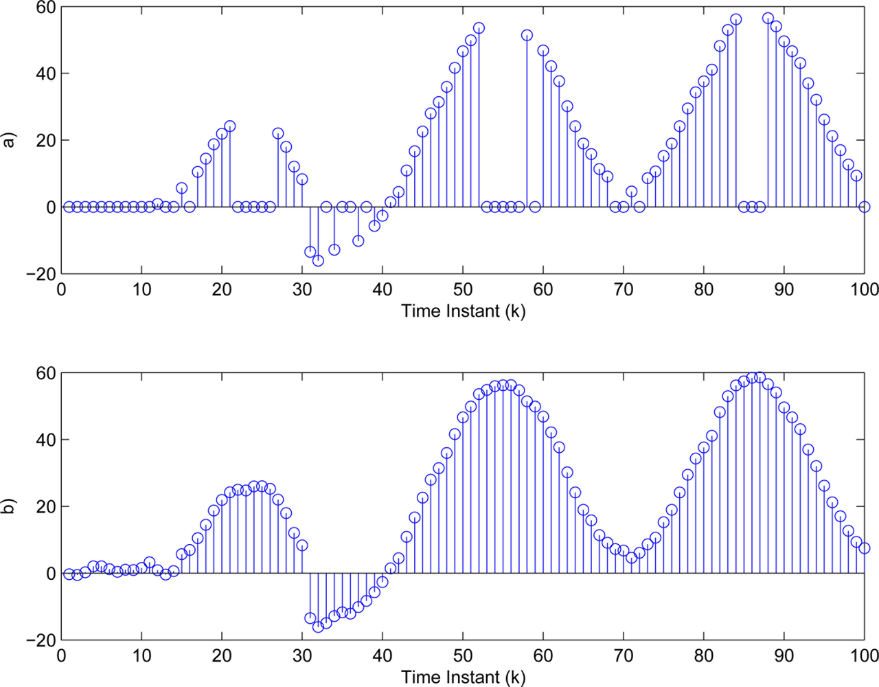
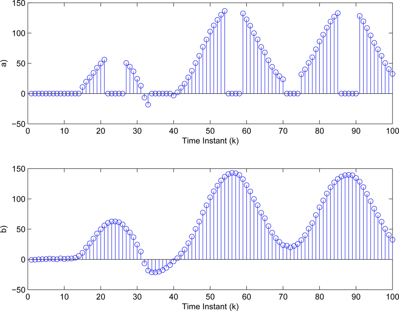
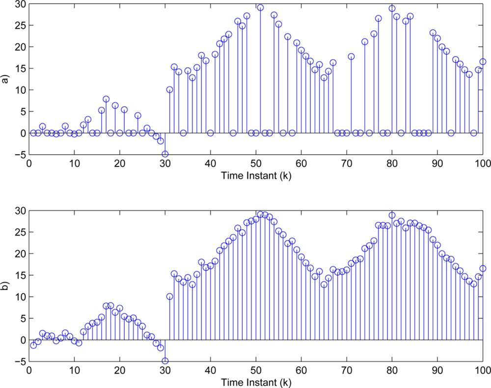
Furthermore, we choose 1 30-fold of the maximal amplitude of y k i (i = 1,2,3). Then, the threshold values in Equation (3) are determined as δ₁ = 4.8406, δ₂ = 2.0382, δ₃ = 1.0009. The sufficiently small threshold ε_i (i = 1,2,3) in Equation (7) is given as 10⁻⁴. Then, Figure 5(a)–7(a) show all the transmitted measurements of sensors with event-triggered scheme. Figures 5(b)–7(b) indicate all the transmitted measurements of sensors with time-triggered scheme. By comparison, the sensors with event-triggered scheme transmit only 66%, 67%, and 58% of samples produced by time-triggered scheme, respectively. In other words, the resource utilization by the event-triggered scheme can be obtained 34%, 33% and 42% improvement, respectively.

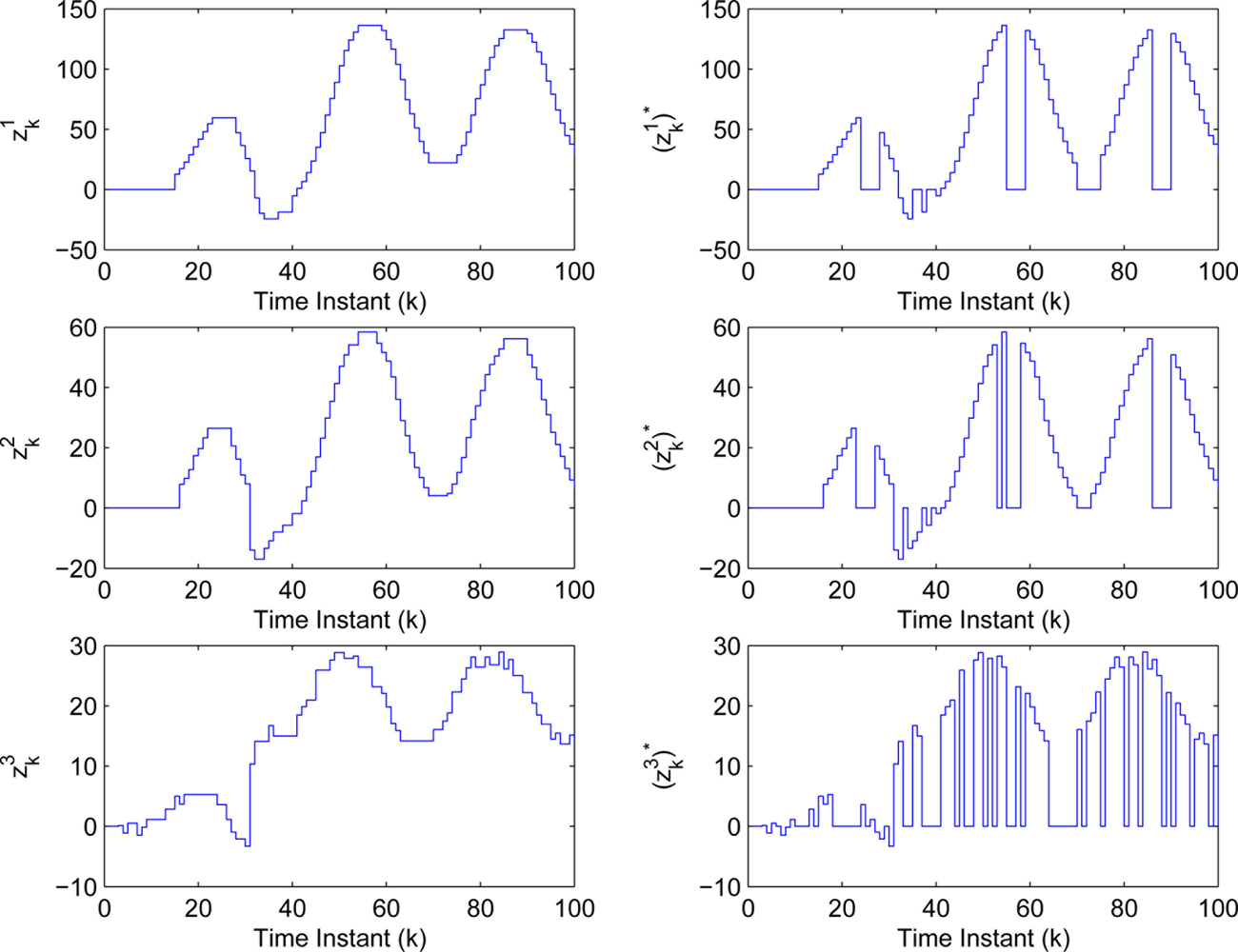
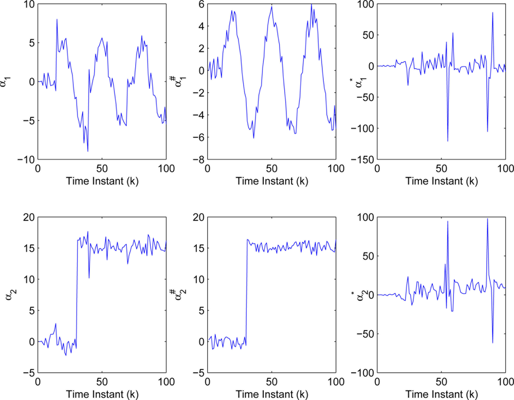
The measurements used in the simulation are indicated in Figure 8, where z k i (i = 1,2,3) and ( z k i ) ★ (i = 1,2,3) represent the measurements with compensating and without compensating some values for the unsent ones, respectively. By Algorithm 1 and the measurements z k i, a modified FIF is implemented to the NCS with event-triggered sampling. Figure 9 shows the innovation sequences of residual α k = [ ( α 1 ) k ( α 2 ) k ] T, α k # = [ ( α 1 # ) k ( α 2 # ) k ] T and α k ★ = [ ( α 1 ★ ) k ( α 2 ★ ) k ] T, which correspond to the residual obtained by the modified FIF described in Algorithm 1, the Keller’s FIF in [27] using the time-triggered samples and the Keller’s FIF using the measurements ( z k i ) ★, (i = 1,2,3), respectively.

In order to compare the simulation results obtained by different schemes, we propose the root mean square (RMS) of the fault estimation errors as a performance index. This error for the scalar variable n_i with respect to its estimate α_i for N_s simulation steps is defined as (17) RMS i ≜ ∑ j = 1 N s [ n i j − α i j ] 2 N swhere n i j is the value of the variable n_i in the jth step, α i j is the estimate of n i j and i = 1,2. Table 1 indicates the RMS of the fault estimation errors by different methods.

From Figure 9 and Table 1, the performance of the modified FIF using less sensor data transmission experiences graceful degradation in contrast to the Keller’s FIF using time-triggered samples. By graceful degradation, it means that a system degenerates in such a manner that it continues to operate, but provides a reduced level of service rather than causing total breakdown. On the other hand, the Keller’s FIF using the measurements ( z k i ) ★ (i = 1,2,3) fails to work completely, while the number of the total sensor data transmission is same as the modified FIF used. From these results, we can draw a conclusion that the modified FIF has an advantage in the tradeoff between communication cost and fault estimation performance.

In order to establish the relationships between the number of the sensor data transmissions, the RMS of the fault estimation errors by different methods and the threshold values δ_i (i = 1,2,3), some further simulations are done by adjusting the threshold values δ_i (i = 1,2,3) from 1/20 to 1/80 of the maximal amplitude of y k i (i = 1,2,3). Figure 10 shows the percentage of transmitted samples to total samples in relation to δ_i by event-triggered scheme, wherein the real line, dash line and dash-dotted line represent the percentage for sensor y k 1, y k 2 and y k 3, respectively. From Figure 10, it can be seen that the sensor data transmission rate is inversely proportional to δ_i, namely the communication cost reduced by the event-triggered scheme will increase when δ_i increases, and vice versa.

In Figure 11, the real line, dash line and dash-dotted line represent the fault estimation performance of the modified FIF, the Keller’s FIF with time-triggered sampling and the FIF with the measurements ( z k i ) ★, respectively. It can be seen that the fault estimation performance of the modified FIF is improved and eventually approaches the performance of Keller’s FIF with time-triggered sampling as δ_i decreases. However, the performance of the FIF with the measurement ( z k i ) ★ (i = 1,2,3) is very poor even by flexibly adjusting the threshold δ_i.

This paper is concerned with the implementation problem of fault isolation filter for networked control system with the send-on-delta scheme which is one of the event-triggered sampling strategies. By send-on-delta, the sensor data is transmitted only when the absolute value of difference between the current sensor value and the previously transmitted one is greater than the given threshold value. Based on this scheme, a modified fault isolation filter for a discrete-time networked control system with multiple faults is then implemented by a particular form of the Kalman filter. In contrast to the Keller’s fault isolation filter using time-triggered samples, the proposed fault isolation filter improves the resource utilization with graceful fault estimation performance degradation. Also, we can improve the performance of the modified FIF by flexibly adjusting the threshold values with taking resource utilization into account.

Throughout the paper, no network-induced packet losses are taken into account in the model of the networked control system. Further study of the fault isolation filter for networked control system with event-triggered sampling and packet losses is encouraged.

References

- Fang, H.; Ye, H.; Zhong, M. Fault diagnosis of networked control systems. Annu. Rev. Control 2007, 31, 55–68. [Google Scholar]
- Aubrun, C.; Sauter, D.; Yame, J. Fault diagnosis of networked control systems. Int. J. Appl. Math. Comput. Sci 2008, 18, 525–537. [Google Scholar]
- Willig, A.; Matheus, K.; Wolisz, A. Wireless technology in industrial networks. Proc. IEEE 2005, 93, 1130–1151. [Google Scholar]
- Domenica, M.; Benedetto, D.; Johansson, K.H.; Johansson, M.; Santucci, F. Industrial control over wireless networks. Int. J. Robust Nonlinear Conr 2010, 20, 119–122. [Google Scholar]
- Miskowicz, M. Send-on-delta concept: An event-based data reporting strategy. Sensors 2006, 65, 49–63. [Google Scholar]
- Suh, Y.S. Send-on-delta sensor data transmission with a linear predictor. Sensors 2007, 7, 537–547. [Google Scholar]
- Kofman, E.; Braslavsky, J.H. Level crossing sampling in feedback stabilization under date-rate constraints. Proceedings of IEEE Conference on Decision and Control, San Diego, CA, USA, 13–15 December 2006; pp. 4423–4428.
- Otanez, P.G.; Moyne, J.R.; Tilbury, D.M. Using deadbands to reduce communication in networked control systems. Proceedings of the 2002 American Control Conference, Anchorage, Ak, USA, 8–10 May 2002; 4, pp. 3015–3020.
- Astrom, K.J.; Bernhardsson, B. Comparison of Riemam and Lebesgue sampling for first order stochastic systems. Proceedings of IEEE Conference on Decision and Control, Las Vegas, NV, USA, 10–13 December 2002; pp. 2011–2016.
- Nguyen, V.H.; Suh, Y.S. Networked estimation with an area-triggered transmission method. Sensors 2008, 8, 897–909. [Google Scholar]
- Miskowicz, M. Efficiency of event-based sampling according to error energy criterion. Sensors 2010, 10, 2242–2261. [Google Scholar]
- Wang, X.; Lemmon, M. Self-triggered feedback control systems with finite-gain L2 Stability. IEEE Trans. Automat. Contr 2009, 45, 452–467. [Google Scholar]
- Lunze, J.; Lehmann, D. A state-feedback approach to event-based control. Automatica 2010, 46, 211–215. [Google Scholar]
- Matveev, A.S.; Savkin, A.V. The problem of state estimation via asynchronous communication channels with irregular transmission times. IEEE Trans. Automat. Contr 2003, 48, 670–676. [Google Scholar]
- Sinopoli, B.; Schenato, L.; Franceschetti, M.; Poolla, K.; Jordan, M.; Sastry, S. Kalman filtering with intermittent observations. IEEE Trans. Automat. Contr 2004, 49, 1453–1464. [Google Scholar]
- Epstein, M.; Shi, L.; Tiwari, A.; Murray, R.M. Probabilistic performance of state estimation across a lossy network. Automatica 2008, 44, 3046–3053. [Google Scholar]
- Schenato, L. Optimal estimation in networked control systems subject to random delay and packet drop. IEEE Trans. Automat. Contr 2008, 53, 1311–1317. [Google Scholar]
- Yook, J.K.; Tilbury, D.M.; Soparkar, N.R. Trading computation for bandwidth: Reducing communication in distributed control systems using state estimators. IEEE Trans. Control Syst. Techn 2002, 10, 503–518. [Google Scholar]
- Xu, Y.; Hespanha, J.P. Estimation under uncontrolled and controlled communications in networked control systems. Proceedings of 44th Conference on Decision and Control, Seville, Spain, 12–15 December 2005; pp. 842–847.
- Xu, Y.; Hespanha, J.P. Communication logics for networked control systems. Proceedings of American Control Conference, Boston, MA, USA, 30 June–2 July 2004; pp. 572–577.
- Xu, Y.; Hespanha, J.P. Optimal communication logics for networked control systems. Proceedings of 43th Conference on Decision and Control, the Bahamas, CA, USA, 17 December 2004; pp. 3527–3532.
- Nguyen, V.H.; Suh, Y.S. Improving estimation performance in networked control systems applying the send-on-delta transmission method. Sensors 2007, 7, 2128–2138. [Google Scholar]
- Nguyen, V.H.; Suh, Y.S. Networked estimation for event-based sampling systems with packet dropouts. Sensors 2009, 9, 3078–3089. [Google Scholar]
- Sijs, J.; Lazar, M. On event based state estimation. Lect. Note Comput. Sci 2009, 5469, 336–350. [Google Scholar]
- Cogill, R. Event-based control using quadratic approximate value functions. Proceedings of IEEE Conference on Decision and Control, Shanghai, China, 15–18 December 2009; pp. 5883–5888.
- Sijs, J.; Lazar, M.; Heemels, W. On integration of event-based estimation and robust MPC in a feedback Loop. Proceedings of International Conference on Hybrid Systems: Computation and Control, Stockholm, Sweden, 12–16 April 2010; pp. 31–40.
- Keller, J.Y. Fault isolation filter design for linear stochastic systems. Automatica 1999, 35, 1701–1706. [Google Scholar]
- Beard, R.V. Failure accommodation in linear systems through self-reorganisation. PhD thesis,. Deptment of Aero-nautics and Astronautics, Massachusetts Institute of Technology, Cambridge, MA, USA, 1971. [Google Scholar]
- Jones, H. Failure detection in linear systems. PhD thesis,. Deptment of Aero-nautics and Astronautics, Massachusetts Institute of Technology, Cambridge, MA, USA, 1973. [Google Scholar]
- Massoumnia, M. A gemetric approachh to the synthesis of failure detection filters. IEEE Trans. Automat. Contr 1986, 31, 839–846. [Google Scholar]
- White, J.; Speyer, J. Detection filter design: Spectral theory and algorithms. IEEE Trans. Automat. Contr 1987, 32, 593–603. [Google Scholar]
- Park, J.; Rizzoni, G. A new interpretation of the fault detection filter: Part 2. Int. J. Contr 1994, 60, 1339–1351. [Google Scholar]
- Liu, B.; Si, J. Fault isolation filter design for time-invariant systems. IEEE Trans. Automat. Contr 1997, 21, 704–707. [Google Scholar]
- Sauter, D.; Li, S.; Aubrun, C. Robust fault diagnosis of networked control systems. Int. J. Adapt. Control Signal Pr 2009, 23, 722–736. [Google Scholar]