This section expresses the sensing methodology of the sensor system; sensors are used to precisely locate an object or pattern of an object using its edges and known locations. For our design we assume frequency information from each of four sensors is from one point of object and each sensor value varies with the distance from the object. The nearer the sensor to the object, the smaller is this frequency value.

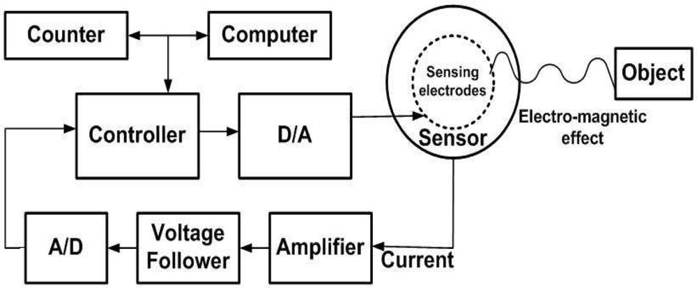
A multiple-element space robot low power sensor with sensing electrodes is used, which is programmed with a proposed sensing algorithm. The capacity type proximity sensor used, comprises a capacitance type sensor, a capacitance type reference, and two independent and mutually opposing driven shields, respectively, adjacent to the sensor and reference and which are coupled in a bridge circuit configuration and driven by a single frequency controlled oscillator [3]. Two mutually opposing driven shields and electro-magnetic effects between the sensing circuit and the sensed object gives rise to a current in the sensors, as shown in Figure 1. Some of the built-in low power sensors, the controller that drives the sensing electrodes, put out a voltage that varies with this current by virtue of the voltage drop of this current across the voltage follower resistor. This voltage follower output is converted to the digital value for control purposes and fed to the controller. The controller of each sensor is capable of transmitting this data to the computer and to the counter so that it can be used by the overall system to guide the robot arm. The controller controls the sensor using feedback through a digital to analog converter. Our controller of the system consists of the Mote circuit board with processor and Tiny OS (operating System) [4]. Section 4 describes in detail the experimental platform used in the testing.

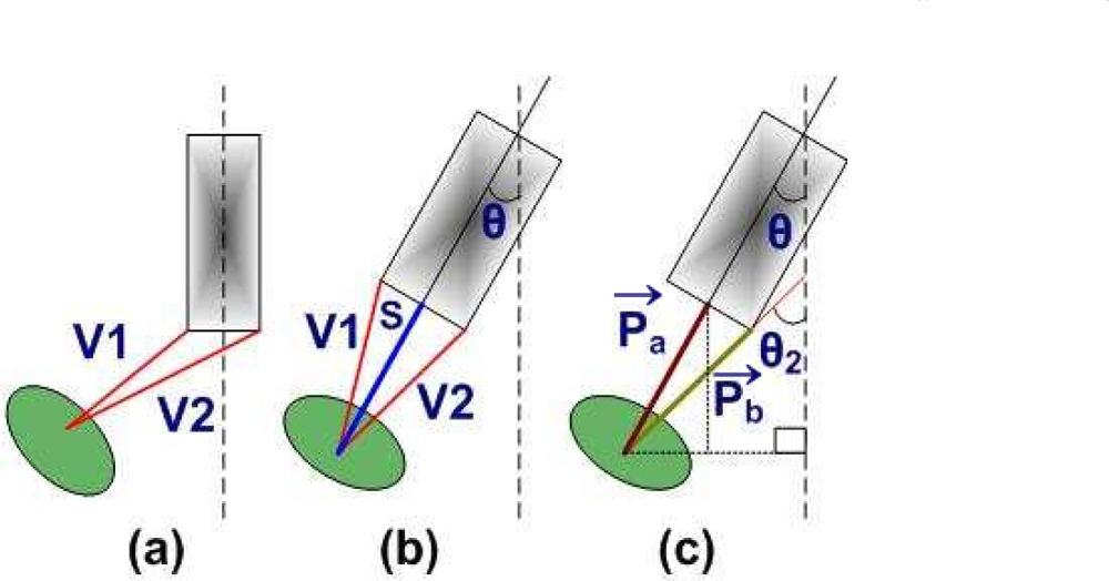
First we think only in 2-D configuration. v1 is sensor1 and v2 is sensor2 known frequency values and current coordinate of sensors are known from hardware feedback. To find an object we increase v1 and decrease v2 till we get the angle θ (direction) and S (required frequency), as shown in Figure 2(b). Figure 2(c) shows that S and is P⃗_a (pattern) and angle θ2 for sensor v2 is P⃗_b (pattern).

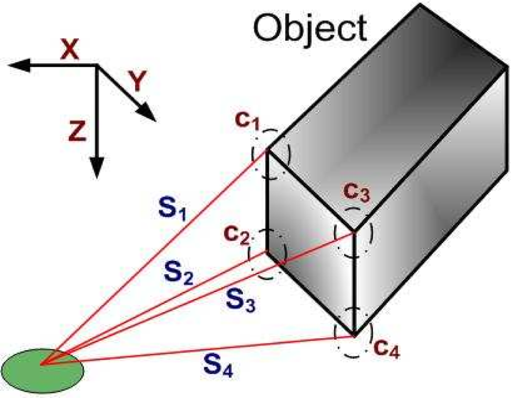
Now we visualize the system in 3-D (as shown in Figure 3). We assume, c₁, c₂, c₃, c₄, and each has the coordinates (x₁, y₁, z₁), (x₂, y₂, z₂), (x₃, y₃, z₃), (x₄, y₄, z₄), respectively. Each sensor has the scalar value S₁ of c₁, S₂ of c₂, S₃ of c₃ and c₄ of S₄. We get the following sets of the equations: (1) ( x 1 − x 0 ) 2 + ( y 1 − y 0 ) 2 + ( z 1 − z 0 ) 2 − S 1 2 = 0 (2) ( x 2 − x 0 ) 2 + ( y 2 − y 0 ) 2 + ( z 2 − z 0 ) 2 − S 2 2 = 0 (3) ( x 3 − x 0 ) 2 + ( y 3 − y 0 ) 2 + ( z 3 − z 0 ) 2 − S 3 2 = 0 (4) ( x 4 − x 0 ) 2 + ( y 4 − y 0 ) 2 + ( z 4 − z 0 ) 2 − S 4 2 = 0where x0, y0, and z0 ≥ 0.

Then, we can find object coordinate using robot arm origin (x₀, y₀, z₀ ) from the above four equations. Now as we know object locations, we can find pattern P⃗_a using Equations (5) and (6): (5) U p a → = ( ( ( x 1 + x 2 + x 3 + x 4 ) 4 − x 0 ) , ( ( y 1 + y 2 + y 3 + y 4 ) 4 − y 0 ) , ( ( z 1 + z 2 + z 3 + z 4 ) 4 − z 0 ) ) = 0 (6) S p a = ( ( ( x 1 + x 2 + x 3 + x 4 ) 4 − x 0 ) 2 , ( ( y 1 + y 2 + y 3 + y 4 ) 4 − y 0 ) 2 , ( ( z 1 + z 2 + z 3 + z 4 ) 4 − z 0 ) 2 ) = 0 (7) P a → = U p a → ⋅ S p a = 0

Based on the pattern P⃗_a, and we can now guide the robot arm in the direction of the object for an accurate positioning. Using one more sensor to detect the object for proper alignment, we can perform the required task by making some rotation and forcing along the z-axis. Also, to clearly explain our methodology, we made a list of 2-D and 3-D configurations as described in Table 1.

The combination of a sensing algorithm with feature recognition requires pre-programmed prior knowledge and operator supervision [5]. The micro energy device’s sensing system consumes low power over the whole electrical system and achieves self- recovery via a sensing manager and a moving manager. When we look at sensors for robots performing precision assembly, an operating principle of the micro energy systems relies on a stable power distribution [6]. We also confirmed that contact surface proximity images can be generated at every sensing step because: (i) the end-unit of the robot is centered and aligned with respect to the fastener; (ii) the electromagnetic effect between the end-unit of robot and fastener can be measured; (iii) the range between the tool and fastener can be calculated from simulation and software models, given the capacitance between them; (iv) each sensors’ surface image is derived from the measurement-adjusted simulation model and displayed in oscillation circuit modeling.

As demonstrated by the profiling result of the combination of multiple sensors (shown in Figure 4), our objective is to minimize the sensing power distribution and moving time. This amounts to maximizing the amount of power distribution that flows a current. Since all array sensors are enclosed by a robot body, they contribute the same to the overall power consumption rate as well as moving time using two software managers—the sensing manager and the moving manager. The specific design application can be implemented for sensor network applications and it will be investigated using an electronic design automation tool, including timing constraints and clock/data frequency recovery circuits under the worst-case scenario. The overall goal of the energy efficient sensor circuit is to model the studied system or plant in robots, to design the control system, and to simulate the entire system by embedding the sensor circuits into the robots. The interface to circuits available in the robots system makes it possible to test the control algorithm with detailed models of all of the hardware components, including piezoelectric sensor, actuators, and devices.

A proposed sensor design gathers information from the environment through measuring mechanical, thermal, chemical, biological, optical, and magnetic phenomena. Moreover, sensor applications and fast data processing are in increasing demand. Energy efficient sensor circuit design also allows for the realistic deployment of highly articulated robots into unknown environments and into environments that are too difficult to model. While carrying on sensors, an issue is extremely important the robot’s ability to determine its location in the world.

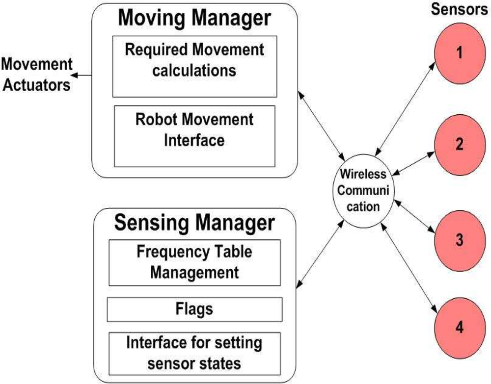
Figure 5 shows how four sensors can detect objects and communicate not only with each other, but also with the managers in our proposed algorithms. We propose a “sensing manager” for controlling the sensors and managing information of each sensor, and a “moving manager” for the actual robot movement.

The four sensors are only needed to read the frequency for a desired object. They send the frequency information to the sensing manger and receive the WAKE or SLEEP commands. Sensors communicate with each other and managers using wireless communication.

The sensing manger has information tables to find the direction and distance of the location. The sensing manager can manage the following tasks and tables:

Each sensors’ maximum frequency table.

The moving manger decides and implements the direction, rotation and movement of the robot. It also performs the tasks below:

Decide first direction pattern (P⃗_a) using four sensors

Our algorithm, which resides in the Tiny OS of our controller, describes how managers work with four sensors in five different modes initial, moving, self-locking, level-setting and forcing. We discuss each mode and its algorithm in detail.

Initialization Mode: This mode sets the start point for the robot and tries to find the first direction or pattern (P⃗_a) of the object by awaking all sensors. This Initialization mode algorithm is as follows:

Algorithm #1
x, y, z = distance (or frequency)
P⃗a = pattern (the vector between four sensors and object)
P⃗b = Near one sensor to the object
init sensing mode{
Set the start point x0, y0, z0
Find the Δx, Δy, Δz
P⃗b = Find Pattern(x, y, z)
}

All the proposed algorithms and techniques were tested using an experimental platform consisting of four mote type boards each mounted with a sensor. The Mica2 mote, developed at UC Berkeley [7] is one of the most popular sensor node designs. It is based on a 7.3 MHz Atmel ATmega128 L embedded controller with 4 Kbytes of RAM and 128 K bytes of ROM. The Mica2 includes a low-power, single-chip radio (the ChipconCC1000) capable of operating at 76.8 kbps with a practical indoor range of approximately 20–30 m. The Mica2 dimensions are 5.7 cm, 3.2 cm, 2.2 cm, and uses two AA batteries that will last for up to a week if the device is powered continuously. However, you can extend its lifetime to months or years through careful duty cycling. The Mica2 runs a specialized operating system, called TinyOS, which addresses the sensor nodes concurrency and resource management [8].

Each board has three parts, as shown in Figure 6, which includes a programming board—MIB510 was used for programming the motes and for housing the base mote for wireless communication. Also, Motes-MICA2 includes a processor that runs the Tiny-OS. It is capable of radio transmission and reception. It has a 51-pin connector for housing the sensor. Finally, Sensors-MTS300 has the capability to sense data and transmits it using the processor/radio module. We have programmed the board using nesC language. Board communicate with the UNIX based PC using serial communication.

For analysis and comparison we analyzed three types of output data from the simulation result we performed. One is the figure of merit, Power Delay (PD) Product, which is essentially the energy consumption per cycle and will remain a constant for a specific machine. Second one is Cache Hit Rate, average time to access memory and tells effectiveness of the cache. Third is the Moving time, the time taken by mode to move the robot or actuator.

We have tested the sensor algorithm using the experimental platform and verified it by benchmarking, using Integer Matrix Multiply (IMM) and Vector Matrix Multiplier (VMM) benchmarks on a machine equipped with an Intel Itanium microprocessor. IMM was chosen because it is designed to facilitate comparing, validating, and improving reconfigurable computing systems. It also provides an architecture-independent compilation framework to express each algorithm’s dependencies and to support automatic synthesis, partitioning, and mapping to a reconfigurable computer [9]. VMM analog VLSI implementation function offers the potential of significant benefits in terms of power, volume, and performance compared to a digital implementation for applications involving fixed or slowly varying weights [10]. Also, in digital systems, VMM reduces the truncation errors and improves vector to vector multiplication.

The benchmark results of our approach on efficient energy consumption are shown in Table 2. We observe our approach for distance moved, active time, power consumption and PD Product in all modes. We note that, since moving mode has more PD Product than others, overall our proposed approach depends mainly on the moving mode, so the proposed algorithm will not restrict the attached hardware actuators’ movements.

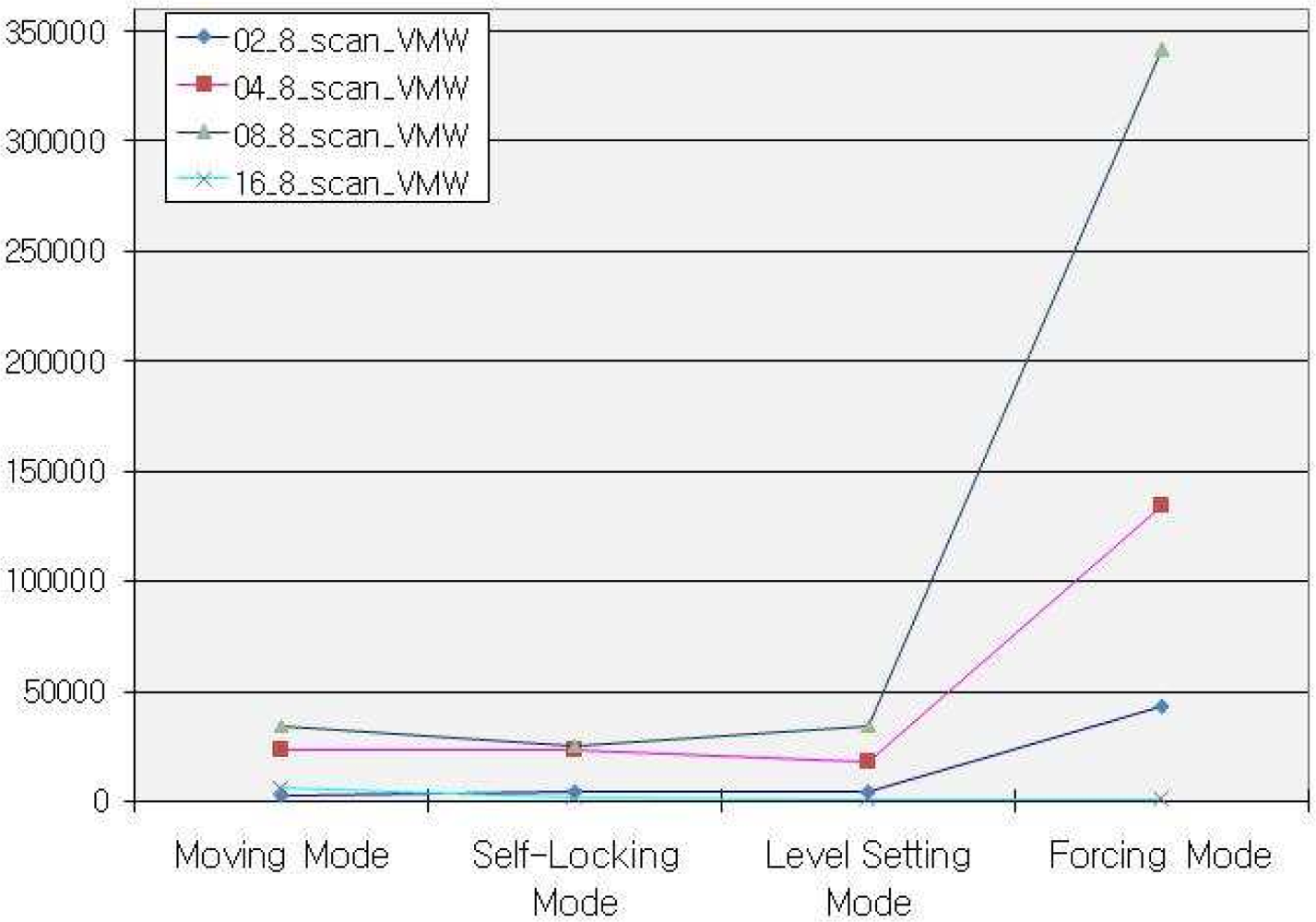
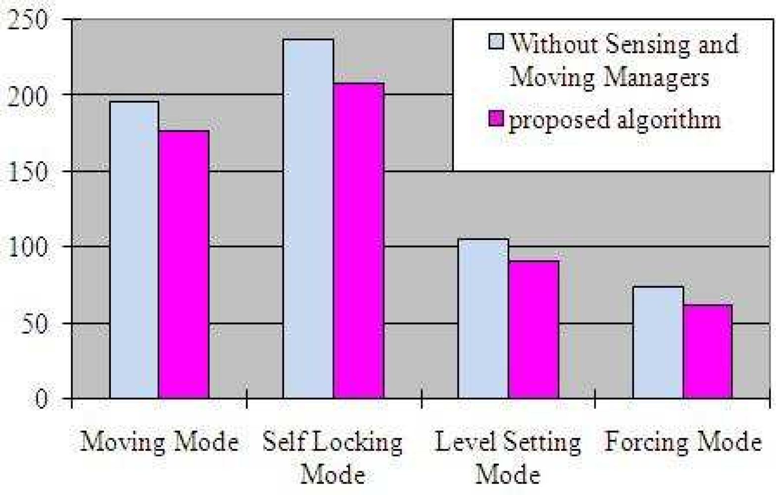
Furthermore, for designing of sensors that have more efficient performance in our approach, we observe the logic gates in Figure 7 used by hardware in each mode by keeping data width 8 and varying the parallel processing nodes and hardware cycles. Figure 8 compares the total time taken in each mode of proposed algorithm with the algorithm lacking the Sensing and Moving manager features.

By studying the two data values of Cache Hit Rate and PD Product, we can predict that our algorithm is energy efficient and has low power consumption. Also, from the values of time taken by each mode we are confident that proposed algorithm has no timing constraints and can also perform well in embedded environment with low speed processors.

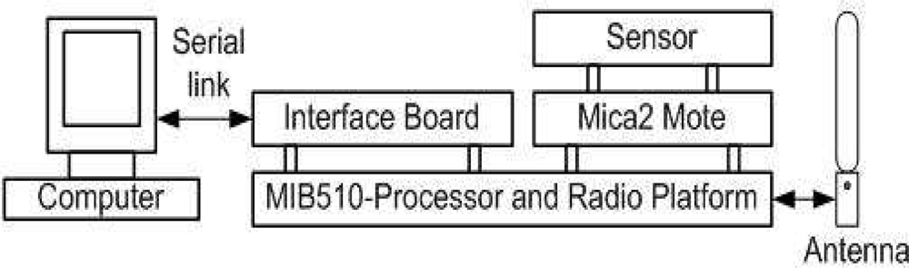
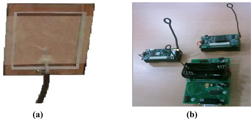
Finally, Figure 9 shows our overall implemented system. Figure 9(a) is a board that included a micro-sensor circuit and Figure 9(b) is a real experimental sensor device, MOTES-MICA2, containing a sensing manger and moving manager. Each sensing and moving manager system was implemented by the embedded board and the robot arm has four sensors. Then the sensing and moving manager system communicates with frequency to the four sensors, and acquires the moving distance, required power consumption, and execution cycle. To precisely adapt the proposed system as well as sensing algorithm, we confirmed that sensor circuits are made by private companies and other defense related industries, e.g., Department of Defense and Aerospace companies. Note that this proposed system could not only be applied to a robot arm, but could also be implemented to many other human environments such as “ubiquitous cities”, “smart homes”, and Wireless Sensor Networks (WSNs), etc.