Detecting Abnormal Vehicular Dynamics at Intersections Based on an Unsupervised Learning Approach and a Stochastic Model

Abstract
:1. Introduction
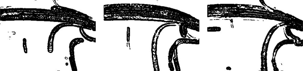
2. Motion Coding
3. Learning States Based on Viscous Morphological Reconstruction
3.1. Binary Spaces with High Dimensionality
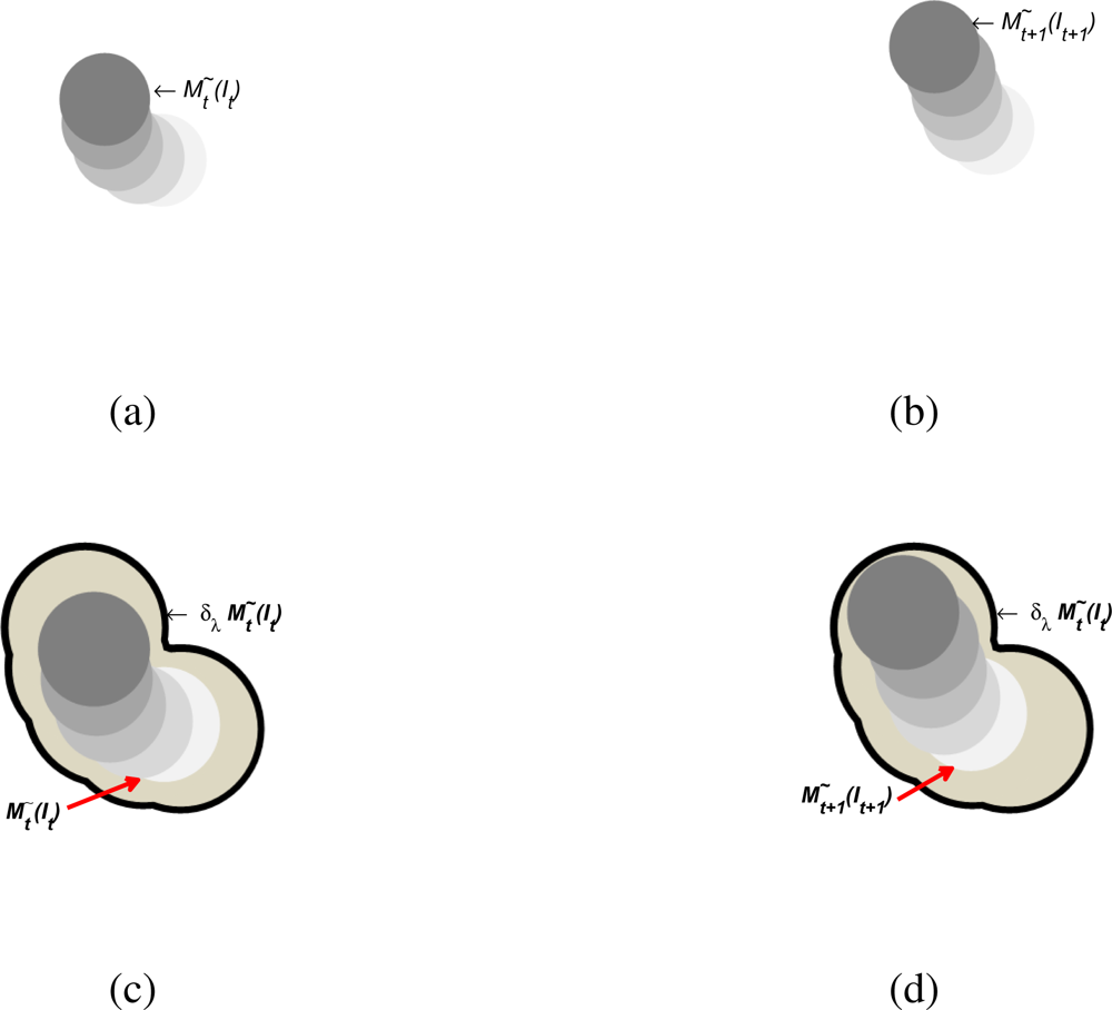
3.2. Morphological Viscous Consistency
3.3. Similarity Measure and Learning Scheme
3.4. Motion Patterns States
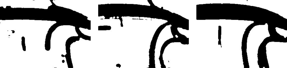
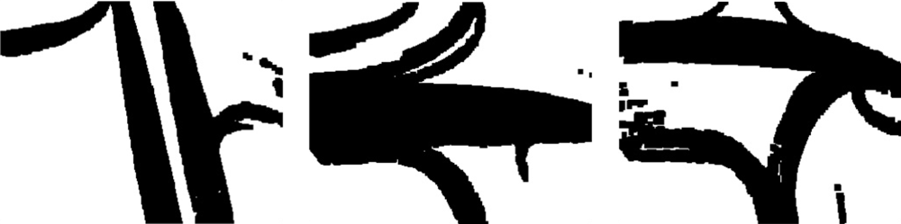
3.5. Abnormal Motion Detection
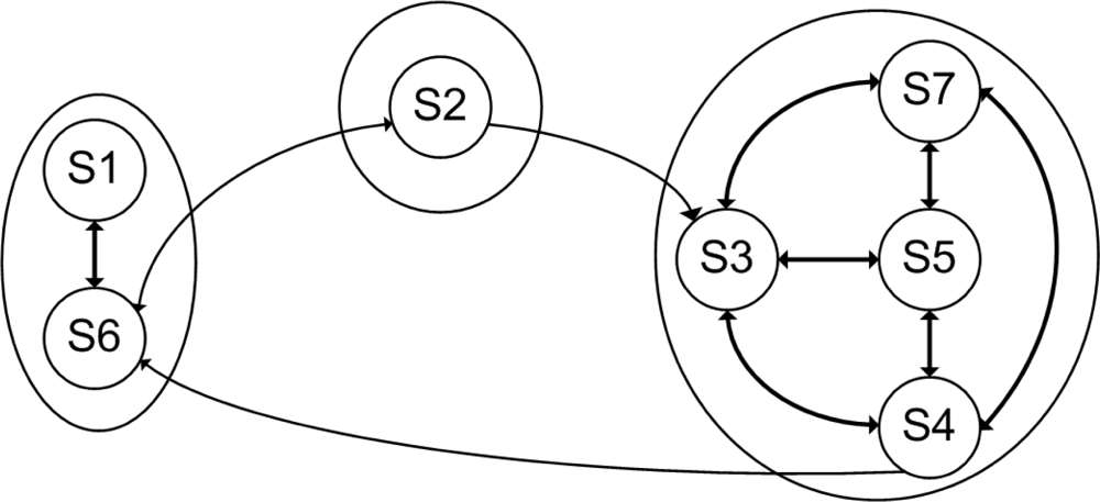
4. Temporal Model
5. Experimental Model and Results
5.1. Experimental Model
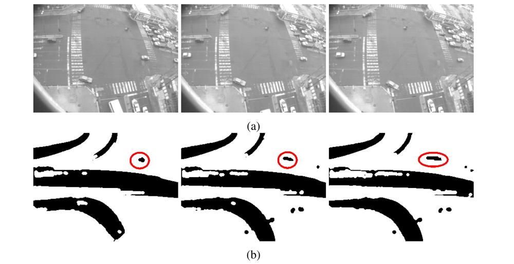
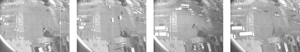
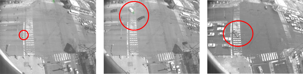
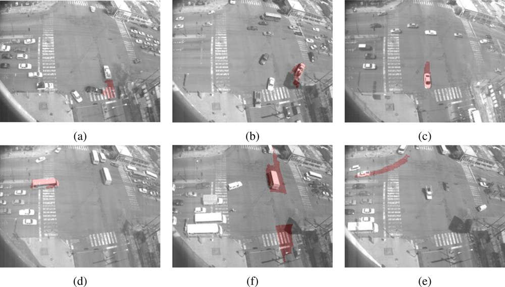
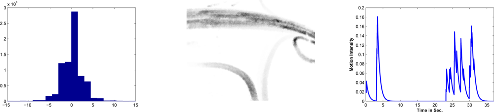
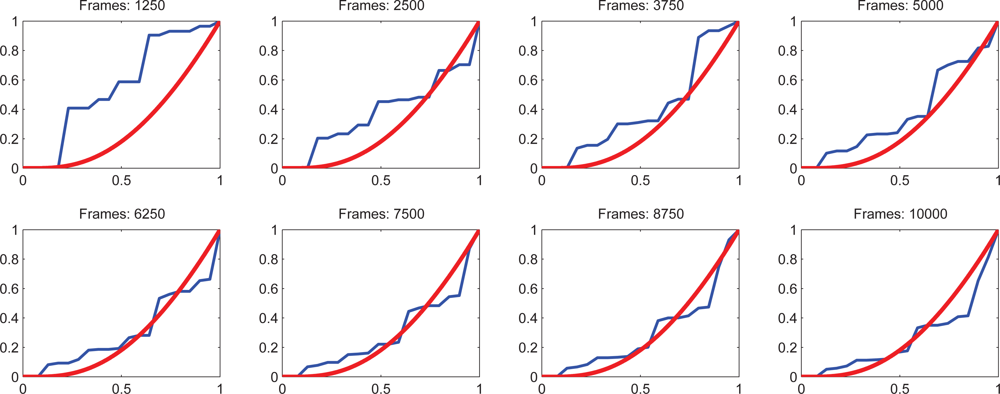
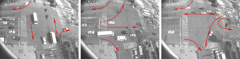
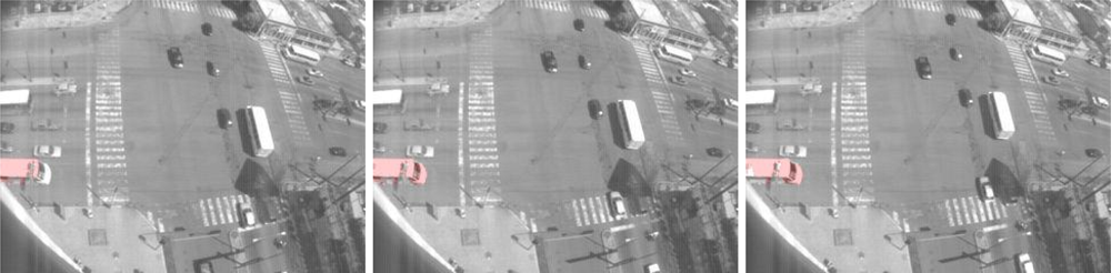
5.2. Analysis of Results
6. Conclusions
Acknowledgments
References
- Collins, RT; Lipton, AJ; Kanade, T; Fujiyoshi, H; Duggins, D; Tsin, Y; Tolliver, D; Enomoto, N; Hasegawa, O; Burt, P; Wixson, L. LambertWixson A System for Video Surveillance and Monitoring; Technical report; Carnegie Mellon University: Cambridge, MA, USA, 2000. [Google Scholar]
- Buxton, H. Advanced Visual Surveillance using Bayesian Networks. IEEE Colloq. Image Process. Secur. Appl 1997, 9, 1–5. [Google Scholar]
- Kanade, T; Collins, R; Lipton, A. Advances in Cooperative Multi-Sensor Video Surveillance; Technical report; Carnegie Mellon University and Stanford Corporation, IEEE Computer Society: Washington, DC, USA, 1997. [Google Scholar]
- Oliver, N; Rosario, B; Pentland, A. A bayesian computer vision system for modeling human interactions. IEEE Trans. Patt. Anal. Mach. Int 2000, 22, 831–843. [Google Scholar]
- Rao, C; Shah, M; Syeda-Mahmood, T. Action Recognition based on View Invariant Spatio-Temporal Analysis. Proceedings of the 11th International Conference on Multimedia (ACM Multimedia 2003), Berkeley, CA, USA, 2–8 November 2003.
- Lou, J; Liu, Q; Hu, W; Tan, T. Semantic Interpretation of Object Activities in a Surveillance System. IEEE Int. Conf. Patt. Recog 2002, 3, 30777. [Google Scholar]
- Hu, W; Hu, M; Zhou, X; Tan, T; Lou, J; Mayobank, S. Principal axis-based correspondence between multiple cameras for people tracking. IEEE Trans. Patt. Anal. Mach. Int 2006, 26, 663–662. [Google Scholar]
- Shannon, C; Weaver, W. The mathematical theory of communication. Bell Syst.Tech. J 1948, 27, 379–423. [Google Scholar]
- Burgin, M. Generalized kolmogorov complexity and duality in theory of computations. Notic. Russ. Acad. Sci 1982, 25, 19–23. [Google Scholar]
- Chaitin, GJ. Algorithmic information theory. IBM J. Res. Dev 1977, 21, 350–359. [Google Scholar]
- Mackay, D. Information Theory, Inference, and Learning Algorithms; Cambridge University Press: Cambrige, UK, 2003. [Google Scholar]
- Brand, M; Kettnaker, V. Discovery and segmentation of activities in video. IEEE Trans. Patt. Anal. Mach. Int 2000, 22, 844–851. [Google Scholar]
- Tomasi, C; Shi, J. Good features to track. Proceedings of Conference on Computer Vision and Pattern Recognition, Seattle, WA, USA, 27 June–2 July 1994; pp. 593–600.
- Lucas, B; Kanade, T. An iterative image registration technique with an application to stereo vision. Proceedings of the DARPA Proceedings on Image Understanding Workshop, Washintong, DC, USA, April 1981; pp. 674–679.
- Lopes, R; Reid, I; Hobson, P. The two-dimensional Kolmogorov-Smirnov test. Proceedings of XI International Workshop on Advanced Computing and Analysis Techniques in Physics Research, Amsterdam, the Netherlands, 23–27 April 2007.
- Dempster, A; Laird, N; Rubin, D. Maximum likelihood from incomplete data via the EM algorithm. J. Royal Stat. Soci 1977, 39, 1–38. [Google Scholar]
- Park, JM; Lu, Y. Edge detection in grayscale, color, and range images. Wiley Encyclopedia Comput Sci Engin 2008. [Google Scholar] [CrossRef]
- Soille, P. Morphological Image Analysis: Principles and Applications; Springer-Verlag: Berlin, Germany, 1999. [Google Scholar]
- Kanerva, P. Sparse Distributed Memory; MIT Press: Cambridge, MA, USA, 1998. [Google Scholar]
- Santini, S; Jain, R. Similarity measures. IEEE Trans. Patt. Anal. Mach. Int 1999, 21, 871. [Google Scholar]
- Braga-Neto, U; Goutsias, J. A theoretical tour of connectivity in image processing and analysis. J. Math. Imaging Vision 2003, 19, 5–31. [Google Scholar]
- Barron, J; Fleet, D; Beauchemin, S; Burkitt, T. Performance of optical flow techniques. Proceedings of IEEE Conference on Computer Vision and Pattern Recognition, Champaign, IL, USA, 15–18 June 1992; pp. 236–242.
- Tsutui, H; Miura, J; Shirai, Y. Optical flow-based person tracking by multiple camera. Proceedings of IEEE Multisensor Fusion and Integration for Intelligent Systems, Kauai, HI, USA, 20–22 August 2001; pp. 91–96.
- Fleet, D; Weiss, Y. Optical flow estimation. In Handbook of Mathematical Models in Computer Vision; Springer: Berlin, Germany, 2006. [Google Scholar]
- Serra, J. Viscous Lattices; Technical report; Centre de Morphologie Mathématique Ecole National Superiure des Mines Paris, 35; rue Saint-Honor: Paris, France, 2004. [Google Scholar]
- Wolpert, DH. The supervised learning no-free-lunch theorems. Proceedings of the 6th Online World Conference on Soft Computing in Industrial Applications, On the World Wide Web. 10–24 September 2001.
- Porikli, F. Trajectory pattern detection by HMM parameter space features and eigenvector Clustering. Proceedings of 8th European Conference on computer vision (ECCV), Prague, Czech Republic, 11–14 May 2004.
- Nguyen, N; Phung, D; Venkatesh, S; Bui, H. Learning and detecting activities from movement trajectories using the hierarchical hidden markov models. IEEE Conf. Comput. Vision Patt. Recog 2005, 2, 955–960. [Google Scholar]
- Baum, LE; Petrie, T; Soules, G; Weiss, N. A maximization technique occurring in the statistical analysis of probabilistic functions of Markov chains. Ann. Math. Statist 1970, 41, 164–171. [Google Scholar]
- Quine, WVO. Notes on Existence and Necessity. J. Phil 1943, 40, 113–127. [Google Scholar]
Appendix—Metric Proof
- ; using a pair of binary patterns and , we have thatNext, making the substitution of the first one into the second one we have that . Perhaps, under the identity of indiscernibles [30], we conclude that iff .
- ; using contradiction proof it is clear thatis true, but, and then Equation (20) becomes false, consequently is true.
- ; expanding each term and grouping show thatTo simplify, it was assumed that the cardinality of each be the same. Left side of the expression have three cases, when patterns are completely non-overlapped, completely overlapped, or partial overlapped.
- When they are completely non-overlapped, the left side can be rewritten as and right side similarly is rewritten as , which becomes true.
- When they are completely non-overlapped, the left side can be rewritten as and right side similarly is rewritten as , which becomes true.
- When they are partially overlapped and right side similarly is rewritten as , which becomes true.
- ; for a given pair of binary patterns and , we have that . Then the expression is true only when and become totally disjoint, that is, for a particular binary pattern , must be ; i.e., .
- ; which is true in sense .
- ; expanding each term and grouping reveals:which is true when they are completely non-overlapped because and . As the same way, is true when are full overlapped because . When they are partially overlapped right side become maxima, when , at right side first almost be equal than because has the same cardinality.


| Approach | Derivative Approximation |
|---|---|
| Convolution Mask | Simple Derivative. |
| Sobel Mask. | |
| Prewitt Mask. | |
| Laplacian Mask. | |
| Roberts Mask. | |
| Deriche Mask. | |
| Morphological Operator | Inner Derivative. |
| Outer Derivative. | |
| Parameter | Values |
|---|---|
| Motion Coding | |
| ∇ | Sobel Mask |
| ρ1 | 1 − (0.1n)−1* |
| ρ2 | 1− (0.1n)−1* |
| ρ | 1 − (5 * f ps)−1** |
| λd | kσ for k = 3 |
| Learning States | |
| λ1 | disk of 3 size |
| λ2 | disk of 5 size |
| λth | |
| KSconf | 0.90 |
| λp | 0.01 |
| Description | Number of Events |
|---|---|
| Events recognized as Abnormal | 9 |
| Events non recognized as an states | 8 |
| Events not parsed | 29 |
| Description | Number |
|---|---|
| Abnormal events detected | 983 frames |
| Non-Recognized states | 587 frames |
| Non-Recognized sequences of states | 307 states transitions |
© 2010 by the authors; licensee MDPI, Basel, Switzerland. This article is an open access article distributed under the terms and conditions of the Creative Commons Attribution license (http://creativecommons.org/licenses/by/3.0/).
Share and Cite
Jiménez-Hernández, H.; González-Barbosa, J.-J.; Garcia-Ramírez, T. Detecting Abnormal Vehicular Dynamics at Intersections Based on an Unsupervised Learning Approach and a Stochastic Model. Sensors 2010, 10, 7576-7601. https://doi.org/10.3390/s100807576
Jiménez-Hernández H, González-Barbosa J-J, Garcia-Ramírez T. Detecting Abnormal Vehicular Dynamics at Intersections Based on an Unsupervised Learning Approach and a Stochastic Model. Sensors. 2010; 10(8):7576-7601. https://doi.org/10.3390/s100807576
Chicago/Turabian StyleJiménez-Hernández, Hugo, Jose-Joel González-Barbosa, and Teresa Garcia-Ramírez. 2010. "Detecting Abnormal Vehicular Dynamics at Intersections Based on an Unsupervised Learning Approach and a Stochastic Model" Sensors 10, no. 8: 7576-7601. https://doi.org/10.3390/s100807576
APA StyleJiménez-Hernández, H., González-Barbosa, J.-J., & Garcia-Ramírez, T. (2010). Detecting Abnormal Vehicular Dynamics at Intersections Based on an Unsupervised Learning Approach and a Stochastic Model. Sensors, 10(8), 7576-7601. https://doi.org/10.3390/s100807576