Investigation of the Frequency Shift of a SAD Circuit Loop and the Internal Micro-Cantilever in a Gas Sensor


Abstract
:
1. Introduction
2. Experimental Details
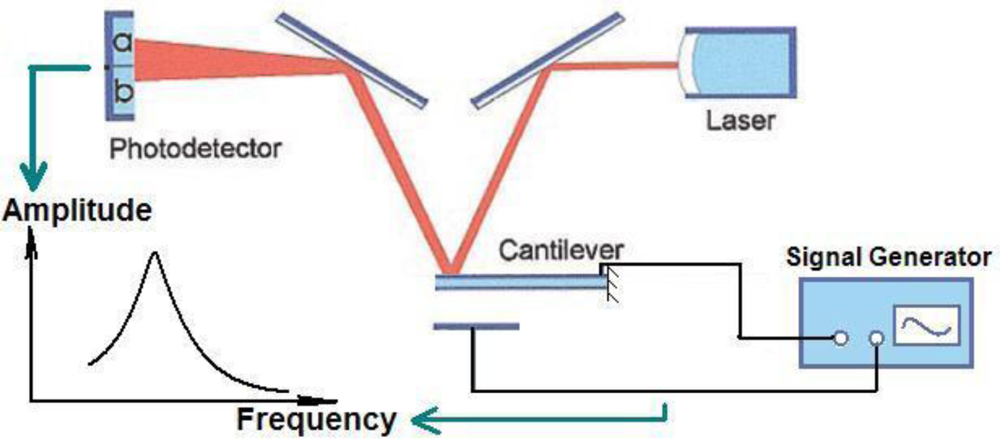
2.1. Brief Description of the SAD Circuit Loop
2.2. Analyte Concentration Controlling
2.3. Open-Loop Tests
2.4. Close-Loop Tests
3. Results and Discussion
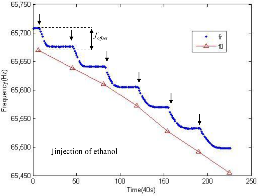
3.1. Initial Offsets
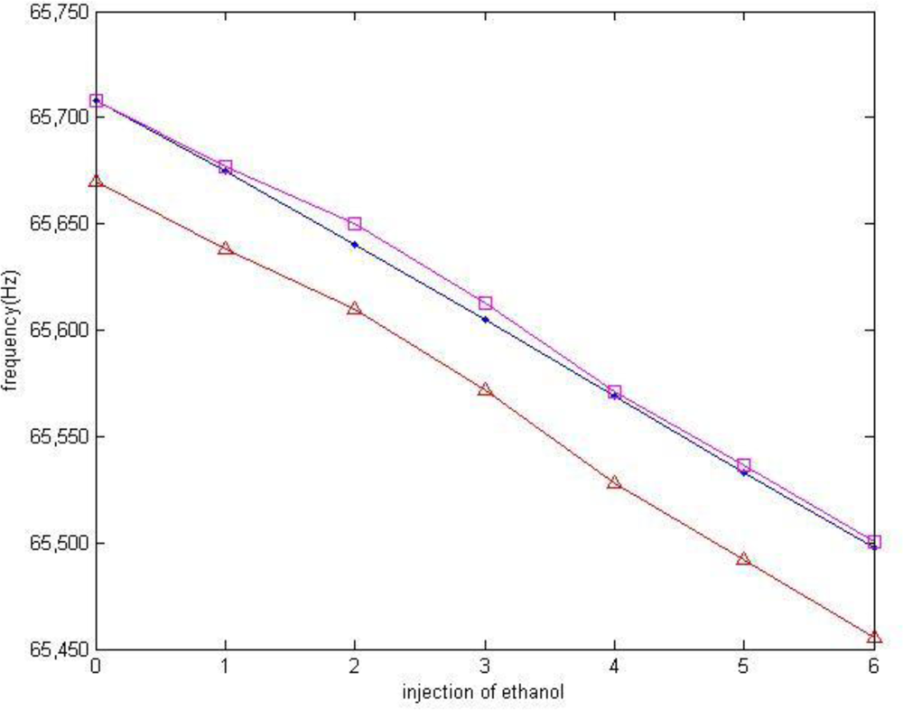
3.2. Differences between MRF Shifts and SWF Shifts
4. Conclusions
Acknowledgments
References
- Zougagh, M; Rios, A. Micro-electromechanical sensors in the analytical field. Analyst 2009, 134, 1274–1290. [Google Scholar]
- Lange, D; Hagleitner, C. Complementary metal oxide Semiconductor cantilever arrays on a single chip: mass-sensitive detection of volatile organic compounds. Anal. Chem 2002, 74, 3084–3095. [Google Scholar]
- Zhou, Q. Study on MEMS chemical gas sensor based on resonating microcantilever. M.S. thesis; Tsinghua University: Beijing, China, 2006. [Google Scholar]
- Li, P; Zhao, J. Resonating frequency of a SAD circuit loop and inner micro-cantilever in a gas sensor. IEEE Sens. J. (In press)
- Datar, R; Kim, S; Jeon, S; Hesketh, P; Manalis, S; Boisen, A; Thundat, T. Cantilever sensors: Nanomechanical tools for diagnostics. MRS Bull 2009, 34, 449–454. [Google Scholar]
- Finot, E; Passian, A; Thundat, T. Measurement of mechanical properties of cantilever shaped materials. Sensors 2008, 8, 3497–3541. [Google Scholar]
- Fadel, L; Lochon, F. Chemical sensing: millimeter size resonant microcantilever performance. J. Micromech. Microeng 2004, 14, S23–S30. [Google Scholar]
- Bedair, S; Fedder, G. CMOS MEMS oscillator for gas chemical detection. Proc. IEEE 2004, 2, 955–958. [Google Scholar]
- Vancura, C; Ruegg, M. Magnetically actuated complementary metal oxide semiconductor resonant cantilever gas sensor systems. Anal. Chem 2005, 77, 2690–2699. [Google Scholar]
- Li, Y; Vancura, C. Monolithic CMOS multi-tranducer gas sensor microsystem for organic and inorganic analytes. Sens. Actuat 2007, B126, 431–440. [Google Scholar]
- Lu, J; Ikehara, T. Characterization and improvement on quality factor of microcantilevers with self-actuation and self-sensing capability. Microelectron. Eng 2009, 86, 1208–1211. [Google Scholar]
- Mutyala, MSK; Bandhanadham, D. Mechanical and electronic approaches to improve the sensitivity of microcantilever sensors. Acta Mech. Sin 2009, 25, 1–12. [Google Scholar]
- Yu, H; Li, X. Resonant-cantilever bio/chemical sensors with an integrated heater for both resonance exciting optimization and sensing repeatability enhancement. J. Micromech. Microeng 2009, 19, 045023. [Google Scholar]
- Rogers, B; Manning, L; Jones, M; Sulchek, T; Murray, K; Beneschott, B; Adames, JD; Hu, Z; Thundat, T; Cavazos, H; Minne, SC. Mercury vapor detection with a self-sensing, resonating piezoelectric cantilever. Rev. Sci. Instr 2003, 74, 4899–4901. [Google Scholar]
- Feng, G. Resonant sensing theory and devices; Tsinghua University Publishing House: Beijing, China, 2008; pp. 25–26. [Google Scholar]
- Gao, W. Study on resonant MEMS gas sensor based on thermally excited micro cantilever; M.S. Thesis; Tsinghua University: Beijing, China, 2008. [Google Scholar]


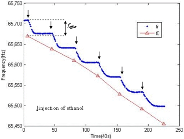
 ]. (b) SWF in close-loop test [
 ]. (c) Simulation results of SWF [
 ].
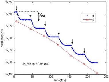
]. (b) SWF in close-loop test [
]. (c) Simulation results of SWF [
].
].
]. (b) SWF in close-loop test [
]. (c) Simulation results of SWF [
].
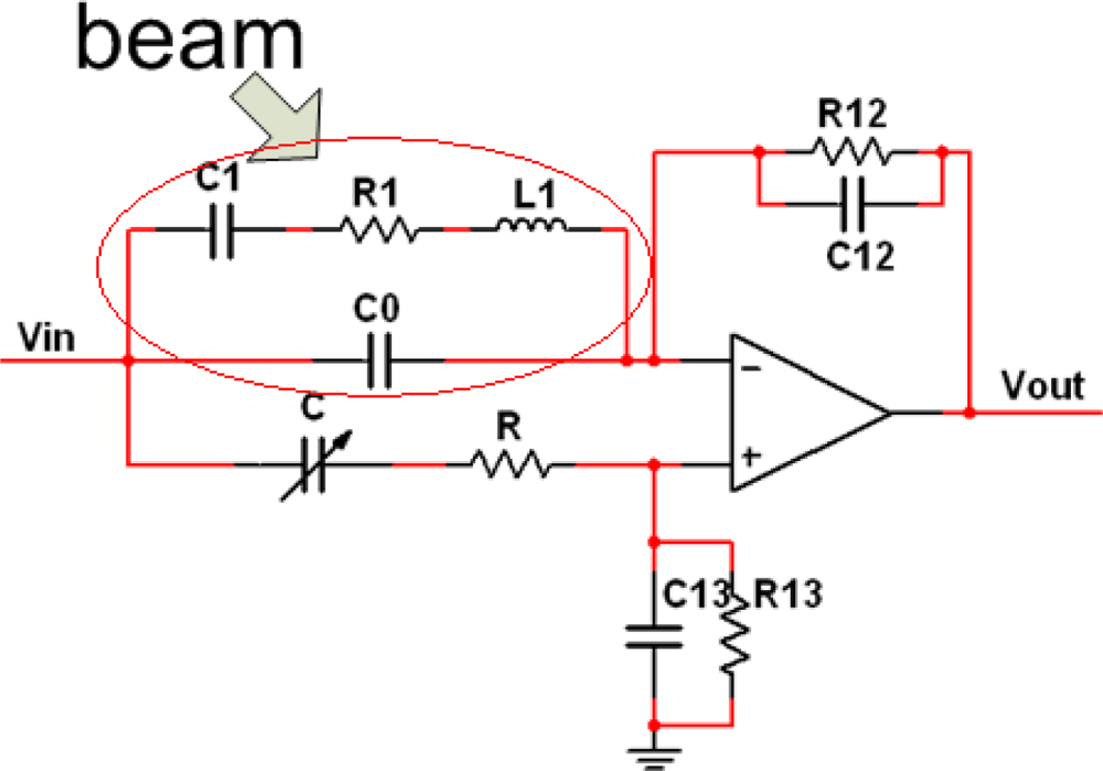
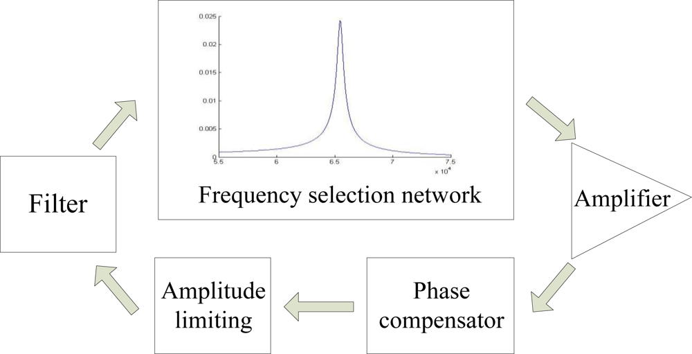
 ], feedback module[
 ] and frequency selection network[
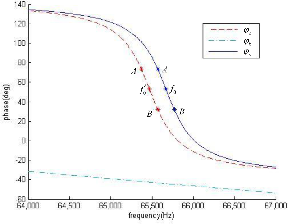
 ]. (b) Experimental measurements of SAD[
 ], feedback module[
 ] and frequency selection network[
 ].
], feedback module[
] and frequency selection network[
]. (b) Experimental measurements of SAD[
], feedback module[
] and frequency selection network[
].
].
], feedback module[
] and frequency selection network[
]. (b) Experimental measurements of SAD[
], feedback module[
] and frequency selection network[
].
© 2010 by the authors licensee MDPI, Basel, Switzerland. This article is an open access article distributed under the terms and conditions of the Creative Commons Attribution license (http://creativecommons.org/licenses/by/3.0/).
Share and Cite
Guan, L.; Zhao, J.; Yu, S.; Li, P.; You, Z. Investigation of the Frequency Shift of a SAD Circuit Loop and the Internal Micro-Cantilever in a Gas Sensor. Sensors 2010, 10, 7044-7056. https://doi.org/10.3390/s100707044
Guan L, Zhao J, Yu S, Li P, You Z. Investigation of the Frequency Shift of a SAD Circuit Loop and the Internal Micro-Cantilever in a Gas Sensor. Sensors. 2010; 10(7):7044-7056. https://doi.org/10.3390/s100707044
Chicago/Turabian StyleGuan, Liu, Jiahao Zhao, Shijie Yu, Peng Li, and Zheng You. 2010. "Investigation of the Frequency Shift of a SAD Circuit Loop and the Internal Micro-Cantilever in a Gas Sensor" Sensors 10, no. 7: 7044-7056. https://doi.org/10.3390/s100707044