L Band Brightness Temperature Observations over a Corn Canopy during the Entire Growth Cycle

Abstract
:1. Introduction
2. Theoretical Background
2.1. Emission from Soil
2.2. Vegetation Effects on Soil Surface Emission
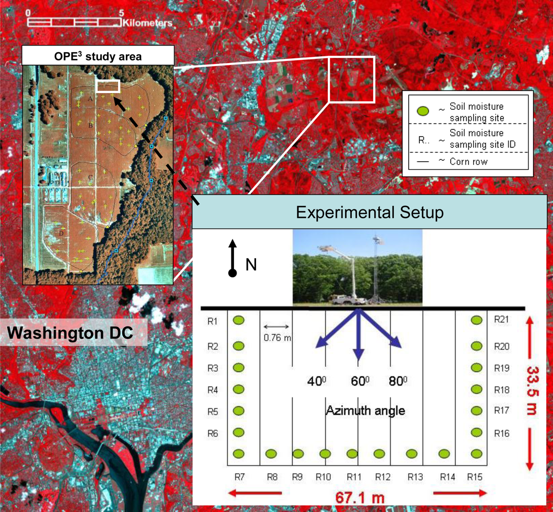
3. The OPE3 Experiment
3.1. Site Description
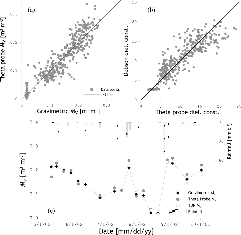
3.2. Ground Measurements
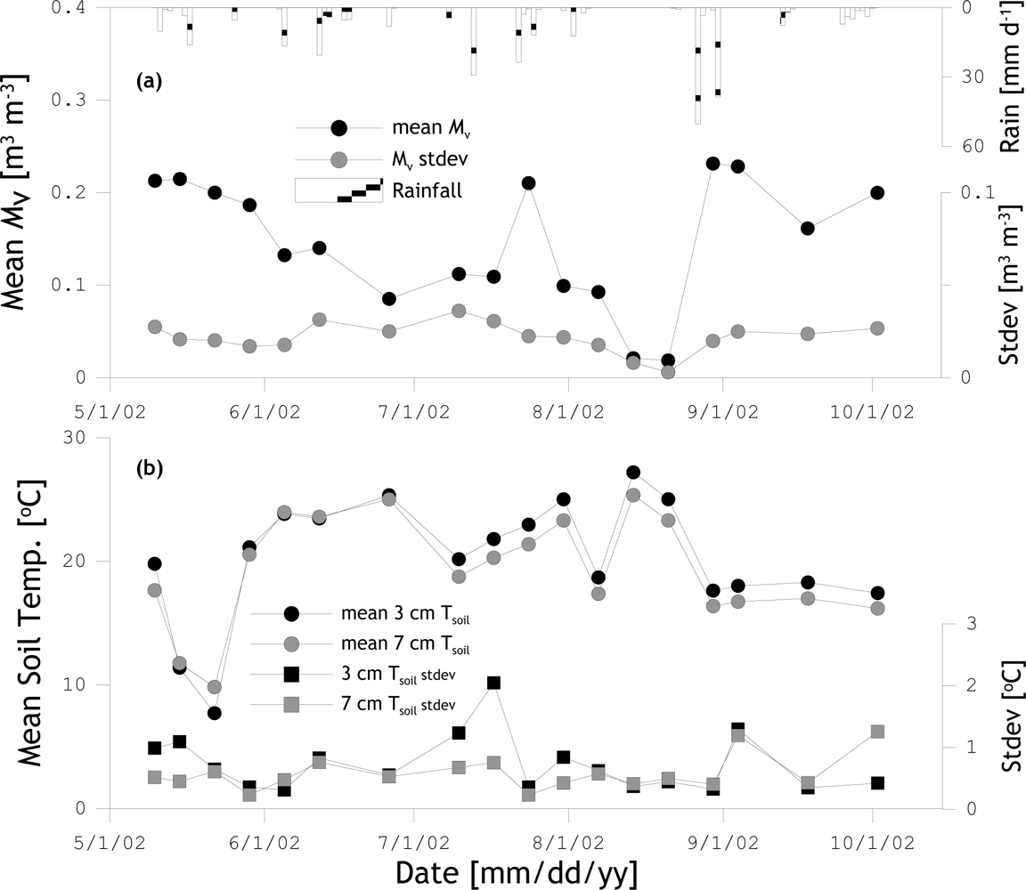
Soil moisture and soil temperature
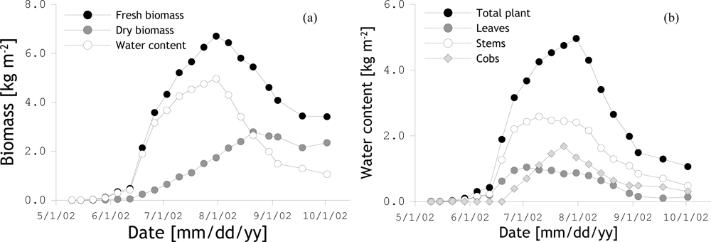
Vegetation
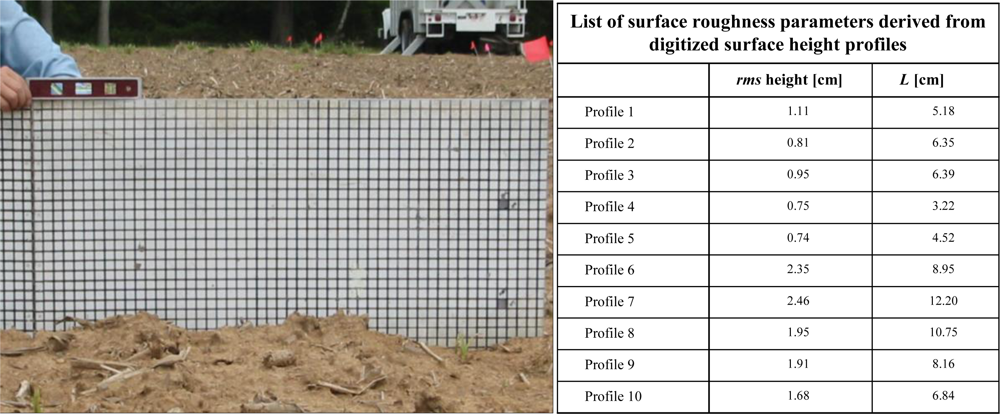
Surface roughness
3.3. Radiometer
4. Results
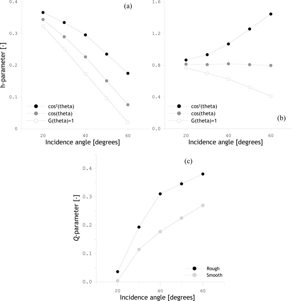
4.1. Surface Roughness Estimation Using H-Polarized TB
4.2. Surface Roughness Parameter Estimation Based on Dual-Polarized TB
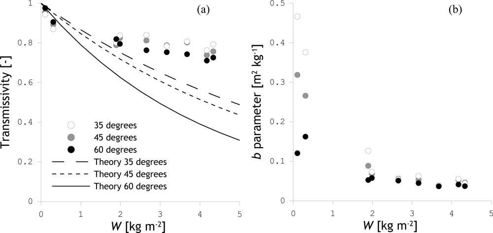
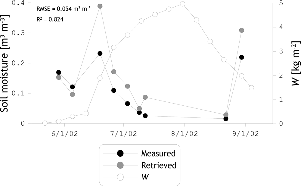
4.3. Estimation of the H-polarized Transmissivity
5. Concluding Remarks
Acknowledgments
References and Notes
- Jackson, TJ. Measuring large scale surface soil moisture using passive microwave remote sensing. Hydrol. Process 1993, 7, 139–152. [Google Scholar]
- Wigneron, JP; Kerr, Y; Waldteufel, P. L-band microwave emission of the biosphere (L-MEB) model: Description and calibration against experimental data sets over crop fields. Remote. Sens. Environ 2007, 107, 639–655. [Google Scholar]
- Owe, M; De Jeu, RAM; Holmes, TRH. Multi-sensor historical climatology of satellite-derived global land surface moisture. J Geophys Res 2008, 113. 1029/2007JF000769. [Google Scholar]
- Saleh, K; Kerr, YH; Richaume, P; Escorihuela, MJ; Panciera, R; Delwart, S; Boulet, G; Maisongrande, P; Walker, JP; Wursteisen, P; Wigneron, JP. Soil moisture retrievals at L-band using a two-step inversion approach. Remote. Sens. Environ 2009, 113, 1304–1312. [Google Scholar]
- Panciera, R; Walker, JP; Kalma, JD; Kim, EJ; Saleh, K; Wigneron, JP. Evaluation of the SMOS L-MEB passive microwave soil moisture retrieval algorithm. Remote. Sens. Environ 2009, 113, 435–444. [Google Scholar]
- Kerr, YH; Waldteufel, P; Wigneron, JP; Martinuzzi, JM; Font, J; Berger, M. Soil moisture retrieval from space: The soil moisture and Ocean Salinity (SMOS) mission. IEEE Trans. Geosci. Remot. Sen 2001, 39, 1729–1735. [Google Scholar]
- Entekhabi, D; Njoku, EG; Houser, P. The Hydrosphere State (Hydros) mission: An Earth system pathfinder for global mapping of soil moisture and land freeze/thaw. IEEE Trans. Geosci. Remot. Sen 2004, 42, 2184–2195. [Google Scholar]
- Jackson, TJ; Le Vine, DM; Hsu, AY; Oldak, A; Starks, PJ; Swift, CT; Isham, JD; Haken, M. Soil moisture mapping at regional scales using microwave radiometry: The Southern Great Plains hydrology experiment. IEEE Trans Geosci Remot Sen 1999, GE-37, 2136–2151. [Google Scholar]
- Owe, M; De Jeu, RAM; Walker, JP. A methodology for surface soil moisture and vegetation optical depth retrieval using the microwave polarization difference index. IEEE Trans. Geosci. Remot. Sen 2001, 39, 1643–1654. [Google Scholar]
- Wen, J; Su, Z; Ma, Y. Determination of land surface temperature and soil moisture from tropical rainfall measuring mission/microwave imager remote sensing data. J. Geophys. Res 2003, 108, 4038–4050. [Google Scholar]
- Pardé, M; Wigneron, JP; Waldteufel, P; Kerr, YH; Chanzy, A; Søbjaerg, SS; Skou, N. N-parameter retrieval from L-band microwave observations acquired over a variety of crop fields. IEEE Trans. Geosci. Remot. Sen 2004, 42, 1168–1178. [Google Scholar]
- Wigneron, JP; Kerr, Y; Waldteufel, P; Saleh, K; Escorihuela, MJ; Richaume, P; Ferrazzoli, P; De Rosnay, P; Gurney, R; Calvet, JC; Grant, JP; Guglielmetti, M; Hornbuckle, B; Mätzler, C; Pellarin, T; Schwank, M. L-band microwave emission of the biosphere (L-MEB) model: Description and calibration against experimental data sets over crop fields. Remote. Sens. Environ 2007, 107, 639–655. [Google Scholar]
- Wigneron, JP; Chanzy, A; Calvet, JC; Bruguier, N. A simple algorithm to retrieve soil moisture and vegetation biomass using passive microwave measurements over crop fields. Remote. Sens. Environ 1995, 51, 331–341. [Google Scholar]
- Jackson, TJ; O’Neill, PE. Attenuation of soil microwave emission by corn and soybeans at 1.4 and 5 GHz. IEEE Trans. Geosci. Remot. Sen 1990, 28, 978–980. [Google Scholar]
- Wigneron, JP; Calvet, JC; De Rosnay, P; Kerr, Y; Waldteufel, P; Saleh, K; Escorihuela, MJ; Kruszewski, A. Soil moisture retrievals from biangular L-band passive microwave observations. IEEE Geosci. Remote. Sens. Lett 2004, 1, 277–281. [Google Scholar]
- Van de Griend, AA; Wigneron, JP. The b-factor as a function of frequency and canopy type at H-polarization. IEEE Geosci. Remote. Sens. Lett 2004, 42, 1–10. [Google Scholar]
- Drusch, M; Wood, EF; Gao, H; Thiele, A. Soil moisture retrieval during the Southern Great Plains Hydrology Experiment 1999: A comparison between experiment remote sensing data and operational products. Water Resour. Res 2004, 40, W2504. [Google Scholar]
- Cashion, J; Lakshmi, V; Bosch, D; Jackson, TJ. Microwave remote sensing of soil moisture: Evaluation of the TRMM microwave imager (TMI) satellite for the Little River Watershed Tifton, Georgia. J. Hydrol 2005, 307, 242–253. [Google Scholar]
- Bindlish, R; Jackson, TJ; Gasiewski, A; Stankov, B; Klein, M; Cosh, MH; Mladenova, I; Watts, C; Vivoni, E; Lakshmi, V; Bolten, J; Keefer, T. Aircraft based soil moisture retrievals under mixed vegetation and topographic conditions. Remote. Sens. Environ 2008, 112, 375–390. [Google Scholar]
- Jackson, TJ; Schmugge, TJ. Vegetation effects on the microwave emission of soils. Remote. Sens. Environ 1991, 36, 203–212. [Google Scholar]
- Schmugge, TJ; Jackson, TJ. A dielectric model of the vegetation effects on the microwave emission from soils. IEEE Trans. Geosci. Remot. Sen 1992, 30, 757–760. [Google Scholar]
- Bindlish, R; Jackson, TJ; Wood, E; Gao, H; Starks, P; Bosch, D; Lakshmi, V. Soil moisture estimates from TRMM Microwave Imager observations over the Southern United States. Remote. Sens. Environ 2003, 85, 507–515. [Google Scholar]
- Saleh, K; Wigneron, JP; De Rosnay, P; Calvet, JC; Escorihuela, MJ; Kerr, Y; Waldteufel, P. Impact of rain interception by vegetation and mulch on the L-band emission of natural grass. Remote. Sens. Environ 2006, 101, 127–139. [Google Scholar]
- Mo, T; Choudhury, BJ; Schmugge, TJ; Wang, JR; Jackson, TJ. A model for microwave emission from vegetation-covered fields. J. Geophys. Res 1982, 87, 11229–11237. [Google Scholar]
- Wang, JR; Choudhury, BJ. Remote sensing of soil moisture content over bare field at 1.4 GHz frequency. J. Geophys. Res 1981, 86, 5277–5282. [Google Scholar]
- Wang, JR; O’Neill, PE; Jackson, TJ; Engman, ET. Multifrequency measurements of the effects of soil moisture, soil texture, and surface roughness. IEEE Trans Geosci Remot Sen 1983, GE-21, 44–51. [Google Scholar]
- Lang, RH; Sidhu, JS. Electromagnetic backscattering from a layer of vegetation: A discrete approach. IEEE Trans. Geosci. Remot. Sen 1983, 21, 62–71. [Google Scholar]
- Chauhan, NS. Soil moisture estimation under a vegetation cover: Combined active passive microwave remote sensing approach. Int. J. Remote. Sens 1997, 18, 1079–1097. [Google Scholar]
- Njoku, EG. AMSR land surface parameters: Surface soil moisture, land surface temperature, vegetation water content. Algorithm Theoretical Basis Documen, Jet Propulsion Laboratory, California Institute of Technology: Pasadena, CA, USA, 1999. [Google Scholar]
- Kerr, YH; Waldteufel, P; Richaume, P; Davenport, I; Ferrazzoli, P; Wigneron, JP. SMOS level 2 processor soil moisture Algorithm Theoretical Basis Document (ATBD). SM-ESL (CBSA), CESBIO, Toulouse,SO-TN-ESL-SM-GS-0001, V5.a, 15/03/2006. 2006. [Google Scholar]
- Gish, TJ; Walthall, CL; Daughtry, CST; Dulaney, WP; Mccarty, GW. Watershed-Scale Sensing of Subsurface Flow Pathways at Ope3 Site. Proceedings of the First Interagency Conference on Research in the Watersheds, Benson, AZ, USA, October 27–30, 2003; pp. 192–197.
- Joseph, AT; Van der Velde, R; O’Neill, PE; Lang, RH; Gish, T. Soil moisture retrieval during a corn growth cycle using L-band (1.6 GHz) radar observations. IEEE Trans. Geosci. Remot. Sen 2008, 46, 2365–2374. [Google Scholar]
- Miller, JD; Gaskin, GD. Theta probe ML2x—Principle of operation and applications, 2nd ed; Macaulay Land Use Research Institute (MLURI): Crairiebuckler, Aberdeen, UK, 1996. [Google Scholar]
- Cosh, MH; Jackson, TJ; Bindlish, R; Famiglietti, JS; Ryu, D. Calibration of an impedance probe for estimation of surface soil water content over large regions. J. Hydrol 2005, 311, 49–58. [Google Scholar]
- Dobson, MC; Ulaby, FT; Hallikainen, MT; El-Rayes, MA. Microwave dielectic behavior of wet soil—Part II: Dielectric mixing models. IEEE Trans Geosci Remot Sen 1985, GE-23, 35–46. [Google Scholar]
- Choudhury, BJ; Schmugge, TJ; Newton, RW; Chang, ATC. Effect of surface roughness on microwave emission of soils. J. Geophys. Res 1979, 84, 5699–5706. [Google Scholar]
- Van de Griend, AA; Wigneron, JP. On the measurement of microwave vegetation properties: Some guidelines for a protocol. IEEE Trans. Geosci. Remot. Sen 2004, 42, 2277–2289. [Google Scholar]
- Wigneron, J; Laguerre, L; Kerr, Y. A simple parameterization of the L-band microwave emission from rough agricultural soils. IEEE Trans. Geosci. Remot. Sen 2001, 39, 1697–1707. [Google Scholar]
- Escorihuela, MJ; Kerr, YH; De Rosnay, P; Wigneron, JP; Calvet, JC; Lemaître, F. A simple model of the bare soil microwave emission at L-band. IEEE Trans. Geosci. Remot. Sen 2007, 45, 1978–1987. [Google Scholar]
- Choudhury, BJ. Reflectivities of selected land-surface types at 19 and 37 GHz from SSM/I observations. Remote. Sens. Environ 1993, 46, 1–17. [Google Scholar]
- Le Vine, DM; Karam, MA. Dependence of attenuation in a vegetation canopy on frequency and plant water content. IEEE Trans Geosci Remot Sen 1996, 34, 1090–1096. [Google Scholar]


| View angle | |||
|---|---|---|---|
| 35 degrees | 45 degrees | 60 degrees | |
| h = h0·cos2 θ | 0.641 | 0.867 | 1.663 |
| h = h0·cos θ | 0.525 | 0.613 | 0.832 |
| h = h0 | 0.429 | 0.434 | 0.416 |
| h = h0·sec θ | 0.352 | 0.307 | 0.208 |
| h = h0·sec2 θ | 0.288 | 0.217 | 0.104 |
| RMSE | |||
|---|---|---|---|
| NRH | h0 | TB [K] | Mv [m3 m−3] |
| NRH = 0.05 (opt.)* | 0.411 | 1.205 | 0.0053 |
| NRH = −2 | 0.104 | 11.225 | 0.0616 |
| NRH = −1 | 0.277 | 6.155 | 0.0074 |
| NRH = 0 | 0.407 | 1.208 | 0.0065 |
| NRH = 1 | 0.613 | 7.441 | 0.0082 |
| NRH = 2 | 0.784 | 13.734 | 0.0074 |
| Date | W | Transmissivity | B parameter | ||||
|---|---|---|---|---|---|---|---|
| kg m−2 | 35° | 45° | 60° | 35° | 45° | 60° | |
| May 29, 2002 | 0.1 | 0.945 | 0.951 | 0.967 | 0.431 | 0.356 | 0.167 |
| June 5, 2002 | 0.3 | 0.857 | 0.878 | 0.881 | 0.423 | 0.306 | 0.211 |
| June 19, 2002 | 1.9 | 0.784 | 0.830 | 0.763 | 0.105 | 0.070 | 0.071 |
| June 26, 2002 | 3.1 | 0.678 | 0.684 | 0.641 | 0.101 | 0.085 | 0.070 |
| July 3, 2002 | 3.7 | 0.695 | 0.679 | 0.629 | 0.081 | 0.075 | 0.063 |
| July 9, 2002 | 4.2 | 0.640 | 0.552 | 0.556 | 0.088 | 0.101 | 0.070 |
| July 12, 2002 | 4.3 | 0.639 | 0.532 | 0.517 | 0.085 | 0.103 | 0.076 |
| August 21, 2002 | 2.6 | 0.783 | 0.758 | 0.736 | 0.078 | 0.076 | 0.060 |
| August 30, 2002 | 2.0 | 0.821 | 0.786 | 0.732 | 0.081 | 0.086 | 0.079 |
| Transmissivity | b-parameter | ||||||
|---|---|---|---|---|---|---|---|
| 35° | 45° | 60° | 35° | 45° | 60° | ||
| May 29th W = 0.1 kg m−2 | TB − 1.0 K | 0.958 | 0.958 | 0.973 | 0.355 | 0.300 | 0.139 |
| TB | 0.949 | 0.951 | 0.967 | 0.431 | 0.356 | 0.167 | |
| TB + 1.0 K | 0.940 | 0.943 | 0.962 | 0.510 | 0.413 | 0.195 | |
| July 9th W = 4.2 kg m−2 | TB − 1.0 K | 0.690 | 0.593 | 0.577 | 0.073 | 0.089 | 0.066 |
| TB | 0.640 | 0.552 | 0.556 | 0.088 | 0.101 | 0.070 | |
| TB + 1.0 K | 0.584 | 0.506 | 0.535 | 0.106 | 0.116 | 0.075 | |
| b-parameter | Single albedo | scattering | |
|---|---|---|---|
| m2 kg−1 | 35° | 45° | 60° |
| 0.10 | 0.014 | 0.017 | 0.033 |
| 0.11 | 0.016 | 0.021 | 0.037 |
| 0.12 | 0.018 | 0.024 | 0.040 |
| 0.13 | 0.020 | 0.027 | 0.043 |
| 0.14 | 0.021 | 0.028 | 0.044 |
| 0.15 | 0.022 | 0.030 | 0.045 |
© 2010 by the authors licensee MDPI, Basel, Switzerland. This article is an open access article distributed under the terms and conditions of the Creative Commons Attribution license (http://creativecommons.org/licenses/by/3.0/).
Share and Cite
Joseph, A.T.; Van der Velde, R.; O’Neill, P.E.; Choudhury, B.J.; Lang, R.H.; Kim, E. J.; Gish, T. L Band Brightness Temperature Observations over a Corn Canopy during the Entire Growth Cycle. Sensors 2010, 10, 6980-7001. https://doi.org/10.3390/s100706980
Joseph AT, Van der Velde R, O’Neill PE, Choudhury BJ, Lang RH, Kim EJ, Gish T. L Band Brightness Temperature Observations over a Corn Canopy during the Entire Growth Cycle. Sensors. 2010; 10(7):6980-7001. https://doi.org/10.3390/s100706980
Chicago/Turabian StyleJoseph, Alicia T., Rogier Van der Velde, Peggy E. O’Neill, Bhaskar J. Choudhury, Roger H. Lang, Edward J. Kim, and Timothy Gish. 2010. "L Band Brightness Temperature Observations over a Corn Canopy during the Entire Growth Cycle" Sensors 10, no. 7: 6980-7001. https://doi.org/10.3390/s100706980