Electromagnet Weight Reduction in a Magnetic Levitation System for Contactless Delivery Applications

Abstract
:1. Introduction
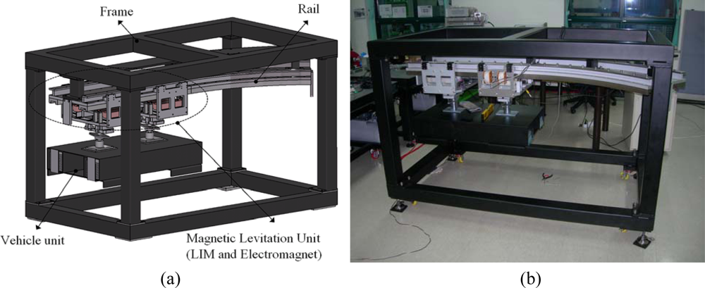
2. Passive Guidance Control and Optimization of Electromagnet
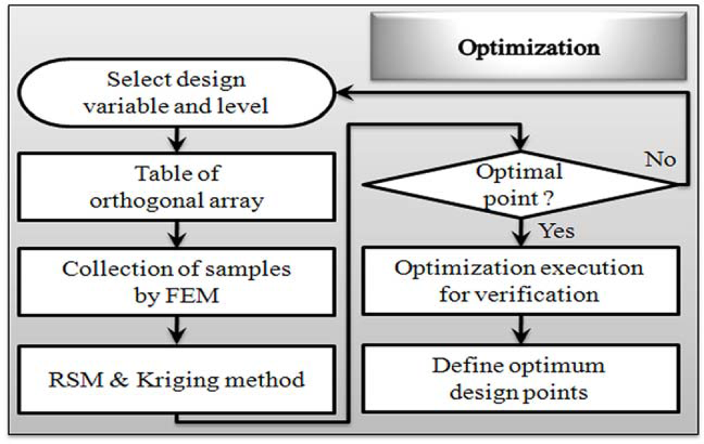
3. Optimum Theory
3.1. Response Surface Methodology
3.2. Kriging Interpolation Method
4. Optimum Design
4.1. Metamodel and Design Variable
4.2. Response Surface Methodology
4.3. Kriging Interpolation Method
5. Conclusions
References
- D’Arrigo, A; Rufer, A. Integrated electromagnetic levitation and guidance system for the swissmetro project. Proceedings of International Conference on Magnetically Levitated Systems and Linear Drives (MAGLEV’ 2000), Rio de Janeiro, Brazil, 7–10 June 2000; pp. 263–268.
- Tzeng, YK; Wang, TC. Optimal design of the electromagnetic levitation with permanent and electro magnets. IEEE Trans. Magn 1994, 30, 4731–4733. [Google Scholar]
- Kim, YJ; Shin, PS; Kang, DH; Cho, YH. Design and analysis of electromagnetic system in a magnetically levitated vehicle, KOMAG-01. IEEE Trans. Magn 1992, 28, 3321–3323. [Google Scholar]
- Onuki, T; Tota, Y. Optimal design of hybrid magnet in Maglev system with both permanent and electromagnets. IEEE Trans. Magn 1993, 29, 1783–1786. [Google Scholar]
- Hong, DK; Woo, BC; Chang, JH; Kang, DH. Optimum design of TFLM with constraints for weight reduction using characteristic function. IEEE Trans. Magn 2007, 43, 1613–1616. [Google Scholar]
- Hong, DK; Choi, SC; Ahn, CW. Robust optimization design of overhead crane with constraint using the characteristic functions. Int. J. Precision Eng. Manuf 2006, 7, 12–17. [Google Scholar]
- Kim, JM; Lee, SH; Choi, YK. Decentralized H∞ control of Maglev systems. Proceedings of IEEE Industrial Electronics, IEEE IECON 2006, Paris, France, 6–10 November 2006; pp. 418–423.
- Lee, KH; Kang, DH. Structural optimization of an automotive door using the kriging interpolation method. Proc. Inst. Mech. Eng. D J. Automobile Eng 2007, 221, 1525–1534. [Google Scholar]
- Guinta, A; Watson, L. A comparison of approximation modeling techniques polynomial versus interpolating models. Proceedings of the 7thAIAA/USAF/NASA/ISSMO Symposium on Multi-disciplinary Analysis and Optimization, Saint Louis, MO, USA, September 1998; pp. 392–440.


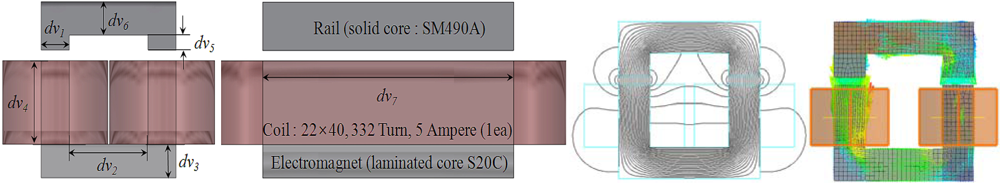
| Design variable Level | dv1 | dv2 | dv3 | dv4 | dv5 | dv6 | dv7 |
|---|---|---|---|---|---|---|---|
| −1 | 16 | 45 | 16 | 40 | 7 | 16 | 144 |
| 0 | 20 | 50 | 20 | 45 | 11 | 20 | 180 |
| 1 | 24 | 55 | 24 | 50 | 15 | 24 | 216 |
| Exp. | dv1 | dv2 | dv3 | dv4 | dv5 | dv6 | dv7 | Normal force (N) | Weight (kg) |
|---|---|---|---|---|---|---|---|---|---|
| 1 | 16 | 45 | 16 | 40 | 7 | 16 | 144 | 382.10 | 8.706 |
| 2 | 16 | 50 | 20 | 45 | 11 | 20 | 180 | 473.67 | 12.153 |
| 3 | 16 | 55 | 24 | 50 | 15 | 24 | 216 | 564.15 | 16.366 |
| 4 | 20 | 45 | 16 | 45 | 11 | 24 | 216 | 682.56 | 15.433 |
| 5 | 20 | 50 | 20 | 50 | 15 | 16 | 144 | 450.22 | 10.979 |
| 6 | 20 | 55 | 24 | 40 | 7 | 20 | 180 | 570.56 | 13.699 |
| 7 | 24 | 45 | 20 | 40 | 15 | 20 | 216 | 795.40 | 16.803 |
| 8 | 24 | 50 | 24 | 45 | 7 | 24 | 144 | 531.60 | 12.66 |
| 9 | 24 | 55 | 16 | 50 | 11 | 16 | 180 | 651.24 | 14.064 |
| 10 | 16 | 45 | 24 | 50 | 11 | 20 | 144 | 379.41 | 10.277 |
| 11 | 16 | 50 | 16 | 40 | 15 | 24 | 180 | 473.76 | 12.094 |
| 12 | 16 | 55 | 20 | 45 | 7 | 16 | 216 | 568.30 | 13.874 |
| 13 | 20 | 45 | 20 | 50 | 7 | 24 | 180 | 570.38 | 13.637 |
| 14 | 20 | 50 | 24 | 40 | 11 | 16 | 216 | 682.15 | 15.453 |
| 15 | 20 | 55 | 16 | 45 | 15 | 20 | 144 | 450.16 | 10.946 |
| 16 | 24 | 45 | 24 | 45 | 15 | 16 | 180 | 659.92 | 14.604 |
| 17 | 24 | 50 | 16 | 50 | 7 | 20 | 216 | 789.93 | 16.646 |
| 18 | 24 | 55 | 20 | 40 | 11 | 24 | 144 | 528.87 | 12.400 |
| Design variable | |||||||
|---|---|---|---|---|---|---|---|
| Model | dv1 | dv2 | dv3 | dv4 | dv5 | dv6 | dv7 |
| Initial | 20 | 50 | 20 | 40 | 15 | 20 | 180 |
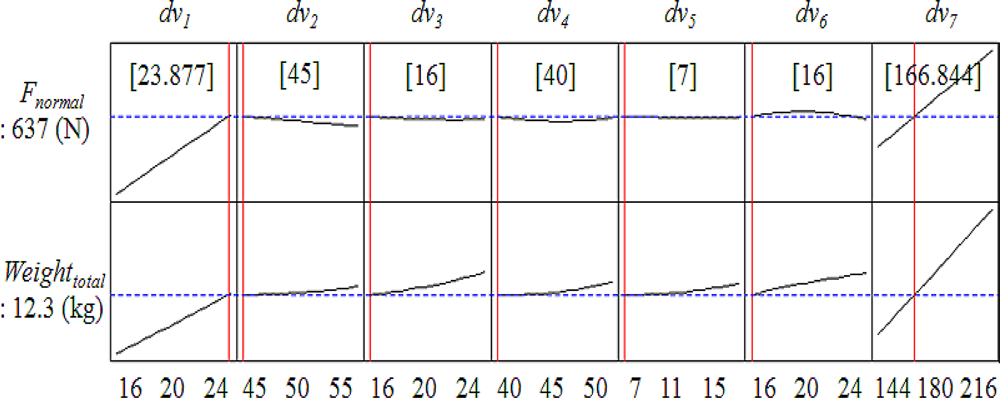
| Optimum (RSM) | 23.877 | 45 | 16 | 40 | 7 | 16 | 166.844 |
| Optimum (Kriging) | 23.877 | 45 | 16 | 40 | 7 | 16 | 166.844 |
| Response | Correlation parameter (corresponding design variable) | |||||||
|---|---|---|---|---|---|---|---|---|
| θ1 (dv1) | θ2 (dv2) | θ3 (dv3) | θ4 (dv4) | θ5 (dv5) | θ6 (dv6) | θ7 (dv7) | β | |
| Weighttotal | 3.026e-3 | 2.304e-4 | 0.909e-3 | 0.201e-3 | 6.318e-5 | 1.195e-3 | 1.289e-2 | 16.0023 |
| Fnormal | 1.319e-2 | 1.382e-5 | 3.437e-6 | 1.172e-5 | 7.819e-6 | 2.320e-6 | 4.087e-2 | 587.009 |
| Model | Weight (kg) | Normal force (N) | |
|---|---|---|---|
| Initial | 2D FEM | 13.319 | 578.5 |
| 3D FEM | 13.319 | 573.48 | |
| Error(2D vs. 3D) % | 0 | 0.86 | |
| Optimum | RSM (predicted) | 12.300 | 637 |
| Kriging method (predicted) | 12.107 | 611.68 | |
| FEM (verification) | 11.799 | 611.70 | |
| Error (RSM vs. FEM) % | −4.073 | −3.972 | |
| Error (Kriging vs. FEM) % | −2.610 | 0.003 | |
| Variation between initial and optimum FEM % | −11.412 | 7.754 | |
© 2010 by the authors licensee MDPI, Basel, Switzerland. This article is an open access article distributed under the terms and conditions of the Creative Commons Attribution license (http://creativecommons.org/licenses/by/3.0/).
Share and Cite
Hong, D.-K.; Woo, B.-C.; Koo, D.-H.; Lee, K.-C. Electromagnet Weight Reduction in a Magnetic Levitation System for Contactless Delivery Applications. Sensors 2010, 10, 6718-6729. https://doi.org/10.3390/s100706718
Hong D-K, Woo B-C, Koo D-H, Lee K-C. Electromagnet Weight Reduction in a Magnetic Levitation System for Contactless Delivery Applications. Sensors. 2010; 10(7):6718-6729. https://doi.org/10.3390/s100706718
Chicago/Turabian StyleHong, Do-Kwan, Byung-Chul Woo, Dae-Hyun Koo, and Ki-Chang Lee. 2010. "Electromagnet Weight Reduction in a Magnetic Levitation System for Contactless Delivery Applications" Sensors 10, no. 7: 6718-6729. https://doi.org/10.3390/s100706718