1. Introduction
Monitoring applications using a single detection device can only obtain local information. If a number of distributed sensors are used to collect data for broader monitored regions or for monitoring tasks with higher precision requirements, and to send those data and perhaps partially processed results to users via mutual collaboration and communication, the information collected by distributed sensor network systems will be more accurate and comprehensive, and the system’s robustness will be stronger. This concept is an important driving force for the development of wireless sensor networks (WSNs).
WSNs are intelligent network application systems that autonomously collect, integrate and transmit data. As an emerging information acquisition technology integrating the latest technological achievements in micro-electronic, network and communications, WSNs have been widely used in many fields such as the military, environmental monitoring, industrial control, and urban transportation [
1]. In comparison to traditional means of environmental monitoring, WSN technology has the following advantages: (1) sensor nodes are small in size and the whole network needs to be deployed only once, so the human impact of the deployment on the monitored environment is very small, which is especially important for environments very sensitive to alien biological activities. Research on the living environment of petrels on the Great Duck Island in the United States showed that even a few minutes of researcher activity on the island would result in a 20% increase in the death rate of fledging birds [
2]; (2) sensor network nodes are large in number, with a high-density distribution, while each node can detect the local environmental information and submit the details to the monitoring center. Sensor networks feature high volume and precision of data acquisition; and (3) wireless sensor nodes have a certain degree of computing power and storage capacity by themselves and can take on more complex monitoring based on changes in the physical environment. Sensor nodes can also communicate wirelessly and monitor collaboratively between nodes.
WSN technology is based on, but different from, the traditional wireless
ad hoc network. The energy of nodes in WSNs is limited, as is their computing, communication and storage capability [
3]. Energy-saving is an essential prerequisite for their reliable operation, and effective energy and resource management has become an important part of the technical issues to be considered, and consequently research on energy consumption has attracted more and more attention [
4].
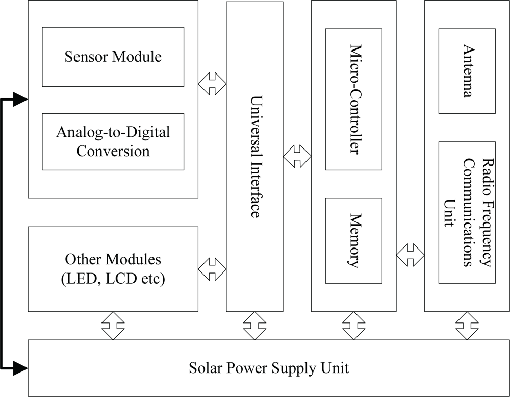
The design of sensor network nodes used for environmental monitoring is shown in
Figure 1. The design features dedicated universal interfaces for common sensors, which can be connected to five types of sensors: water level, precipitation, evaporation, flow and water quality. The circuit of each sensor is designed to be low-power, and its processor can be directed to sleep and wake-up via radio frequency instructions. Meanwhile at the same time sensors are equipped with solar cells to extend their lifetime. With the clustering routing protocol, hydrological information parameters collected within a certain period of time by sensors in a certain number within clusters will be converged to a selected cluster head node. After the fusion treatment, the information will be sent to a sink node and then to a monitoring center via some means of long-distance communication such as GPRS.
From the perspective of network resources, different protocol layers can use different strategies and techniques to meet the energy-saving goal. From the point of view of network layers, many routing protocols are designed and used to improve the network scalability and to extend its network life cycle for WSN applications, such as the energy-based routing protocol [
5], the SPIN negotiation-based routing algorithm [
6], the MTE minimum transmission energy protocol [
7], and the data-centric directed diffusion protocol [
8]. Among them, the routing protocol based on the clustering mechanism is used comparatively more than others [
9].
In a monitored environment with a large-scale deployment of sensor nodes, the monitored properties (such as temperature, humidity, light, wind and precipitation) are usually distributed “structurally” with greater redundancy. Let us consider for example the precipitation distribution of the Taihu Lake Basin, the branch river system in the downstream region of the Yangzi river, centered at Taihu Lake with the drainage channel of the Huangpu river. The river system occupies an area of 36,500 km
2, including Tianmu Mountain in Zhejiang Province and Maoshan Mountain in Jiangsu Province on the west, the end of Yangzi River on the north, facing the East China Sea and Hangzhou Bay on the east and south respectively. The precipitation in the west part of Zhejiang Province (Zhexi, in short) is higher than other areas no matter what year. The precipitation in Pudong and Puxi of Shanghai (a city located at the Coast of East Sea) and Yangcheng Dianmao area of Suzhou City is within the low value area of the precipitation line in every year. That is due to the impact of orographic lift on the precipitation. Zhexi is the only mountain area in the basin while Yangcheng Dianmao is a well-known low-lying land. The spatial distribution of the precipitation in the basin is that it is large in the former and small in the latter. This illustrates the impact of orographic lift on the precipitation. According to years of observation data, the general trend of the precipitation is that the upstream is larger than the downstream, the west than the east, the south than the north and the mountain than the plain in terms of space [
10].
However, from the existing general pattern of precipitation information extraction, it can be seen that the system-level precipitation information processing technology is essentially a background approach of information processing that distributes measuring nodes based on geographical characteristics and processes data centrally. Although the information can be converged after all the data are sent separately to the background, the results obtained from this method are usually not as accurate as those obtained from the fusion in the front, and sometimes even produce fusion error. The participation of local information from the data source is generally required in information fusion, such as time and location of data was generated, and the location generating the data.
The clustering mechanism-based routing protocol [
9] demonstrates its superiority. Its idea is that in a multi-hop communications process, a cluster head is used in data fusion to reduce the amount of data sent to sink nodes and to achieve the purpose of efficient use of energy. Compared with the flat routing protocols (flooding, gossiping,
etc.), the introduction of the clustering mechanism improves performance significantly for similar or dissimilar sensor fusion of data collection with high correlation (or high similarity).
An earlier proposed one is the Low Energy Adaptive Clustering Hierarchy (LEACH) protocol [
11,
12] (referred as the traditional LEACH protocol in this paper). This idea of hierarchy-based protocol design has been accepted by more and more scholars. However there are still some problems in the practice of this routing protocol, the most important of which concerns the unreasonable selection of cluster heads, such as uneven distribution, no regard to the remaining energy of nodes,
etc. Some improved algorithms have been proposed to solve these problems [
13–
15]. However, most of them select cluster heads according to the status information of candidate nodes without considering the information of their neighbors, which tends to result in blind nodes inside clusters, possibly reducing the survival time of the network.
This paper considers monitoring applications for an outdoor environment such as meteorological and hydrological data or the wetland ecology environment, and aims to reduce network energy consumption. It mainly focuses on the optimal selection of cluster heads, improves the traditional LEACH routing algorithm, and introduces and designs a routing algorithm based on the differential evolution algorithm (DE), the DE_LEACH routing algorithm in short. The DE_LEACH algorithm uses the easy and fast search features of the DE in multi-objective optimization applications, takes energy and distance distribution of neighbor nodes inside clusters into account, and then optimizes the selection of cluster heads. The algorithm has advantages in terms of effectively preventing premature blind nodes and reducing network energy consumption, and is more suitable than others to meet the needs of WSN applications in monitoring applications for outdoor environment such as those mentioned before.
The rest of this paper is organized as follows: Section 2 reviews related work on WSN protocols; Section 3 describes the idea of differential evolution algorithms; Section 4 presents the proposed method; Section 5 proves the DE_LEACH algorithm through experiments and analyzes the experiment results, and finally, Section 6 concludes and indicates several issues for future work.
2. Related Work
Currently, there are many network protocols for WSNs with their own advantages and disadvantages. Energy-based routing protocols [
6] can choose transmission paths based on available energy of WSN nodes or energy requirement of links of transmission paths. However, such energy routing algorithms need to know the network global information, and the energy constraints of sensor networks only allows nodes to obtain local information, so they are routing methods just in ideal situations.
A negotiation-based routing algorithm such as the sensor protocol for information via negotiation or SPIN [
7] is a data-centric self-adaptive communication routing protocol. Its goal is to offset the deficiencies in the diffusion method of SPIN through the negotiation mechanism between nodes and the resource self-adaptive mechanism. Its shortcoming is that in the process of new data transmission it directly broadcasts ADV data packages to its neighbor nodes, and that all neighbor nodes are not willing to take the responsibility of forwarding new data due to their own energy. Therefore new data cannot be transferred, data blind spots will appear, and the information collection across the whole network will be affected.
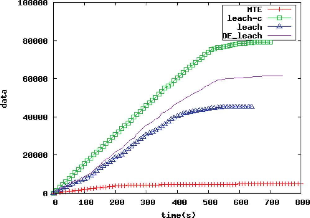
The minimum transmission energy [
8] (MTE) protocol is an improved traditional direct route algorithm. In the MTE, a node chooses the one closest to itself for routing forwarding. Its advantage is simplicity, low cost, and each node only needs to find the next hop node to the sink node, and then sends the data to it. The disadvantage is that sensor nodes near the sink node always takes the role of router, loads between nodes are not in balanced, sensor nodes close to the sink node may soon run out of energy and “die”, and the life cycle of the entire network is shortened.
The Directed Diffusion [
9] protocol is a data-centric routing protocol, and features the introduction of a gradient to describe the possibility of network intermediate nodes continuing their search for matched data along the direction. The disadvantage is that there are no multiple routes to the sink node, and the routing robustness is not good enough.
The LEACH & LEACH_C protocols: LEACH is a cluster-based routing protocol, and uses the following technologies to achieve its energy-saving: 1) random, self-adaptive, self-organization clustering method; 2) local control of data transmission; 3) low-energy consumption of the MAC protocol; 4) information processing technology. The LEACH protocol occupies an important position in WSN routing protocols, and other cluster-based routing protocols have been developed from the LEACH one. Its proposer later improved it, proposing the LEACH_C [
10] protocol. The main improvement was that during the clustering nodes no longer compete for cluster heads, but nodes first send their own data to the sink node, and then the sink node determines the location of cluster heads according to their location, energy and cycle. The advantage of doing so lies in that we get a reasonable distribution of clusters through a reasonable arrangement of cluster heads, reducing the energy consumption due to the non-ideal random location or numbers of clusters in the original LEACH algorithm. For now, the LEACH_C and LEACH protocols may be considered generally equivalent cluster routing protocols.
Nevertheless, the LEACH_C network protocol has its own inherent shortcomings. Because the number of nodes in WSNs is large, the density coverage is also high, and the data collected by a single node are inevitably highly related with those collected by the entire WSN, and what users need is not the data collected by all nodes (including redundant data), but rather a description of incidents—the situation of events taking place in observed regions through the analysis of the set of network.
Taking it into account that the LEACH protocol uses clusters, data sent from nodes is processed locally (compression, de-redundancy) inside clusters and sent to the sink node. This will reduce the dependence of useful information users need on information a certain node collects. It also provides evidence for using the shift rest of nodes to reduce the energy consumption, that is to say, during each working cycle it will not affect the whole system greatly when a small amount of nodes in the network node hibernate.
Based on the above studies, this paper selects part of low energy nodes through cyclical filters, and puts them into the hibernation state to reduce the system’s total energy consumption, to extend the lifetime of the who system. At the same time, it requires consideration of various factors such as energy saving, self-adaptive capability of the network, the accuracy of information in accordance with the characteristics of WSNs when designing WSN protocols.
2.1. Structure Analysis of the Traditional LEACH Protocol
The traditional LEACH routing protocol is a low energy-consumption self-adaptive hierarchical routing algorithm designed for WSNs by Heinzelman
et al. [
9,
11]. Its basic idea is that cluster heads are selected randomly through cycles with equal probability, and integrate and send information collected by members inside clusters to sink nodes to reduce communication traffic and distribute the energy load of the whole network evenly to each sensor node, so as to meet the goal of reducing energy consumption and extending the overall survival time of the network.
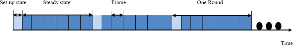
The working process of the LEACH protocol is cyclic, defined as the concept of rounds. In
Figure 2, each round of a cycle is divided into two types of state: set-up state and steady state.
In the set-up state, each sensor node competes for a cluster head at a certain probability and each cluster head broadcasts a message to all nodes that it has become one, and each node determines which one to join based on the signal strength, and responds to that cluster head. In the steady state, the cluster’s members send collected data to the cluster head according to the TDMA time slot, and the head integrates and sends data to sink nodes via Carrier Sense Multiple Access (CSMA). The steady state is much longer than the set-up state, and after a period of working time, the network re-enters a set-up state. The execution process is periodic. From the protocol process, cluster heads need to finish integrating data and communication with sink nodes, so the energy consumption is very high. The LEACH algorithm ensures that each node can be a cluster head in equiprobability, and that each node in the network consumes energy comparatively evenly.
2.2. Problem Description
During the operation process, the traditional LEACH protocol executes the cluster re-construction process constantly in cycles. The re-construction process is described in rounds, and each round needs to create clusters first. The process is mainly about how to select cluster heads. The protocol uses each sensor node to select a random number between 0∼1. If the selected number is less than T(n), then this node becomes a cluster head. This method of selecting cluster heads does not guarantee that cluster head nodes will be distributed over the entire network, and it is very possible for selected cluster heads to concentrate in a certain part of the network, resulting in no cluster heads around some nodes. The phenomenon of uneven distribution of cluster heads may result in premature death of nodes inside clusters, thus becoming blind nodes.
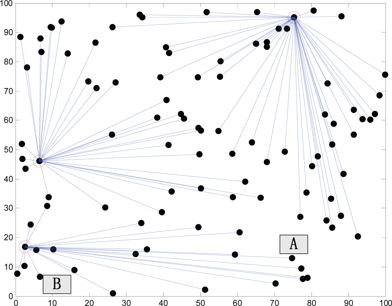
In
Figure 3, nodes A and B belong to the same cluster. Suppose that
R1 is the distance from node A to the cluster head with energy
EA, and
R2 is the distance from node B to the cluster head with energy
EB, and that
EA ≈
EB.
ET, the communications energy, is proportional to the square of the distance to the target [
8], and obviously
EA −
ETA <
EB −
ETB. The margin of the remaining energy increases as the margin between the distances from two nodes to the cluster head increases. If the location of the cluster head is selected improperly, resulting in that the margin between the distances to the cluster head is too large; the uneven level of energy of nodes inside the cluster may be very serious.
The traditional LEACH protocol assumes that all nodes carry the same energy. The selection of cluster heads is regardless to the remaining energy of nodes. However in the actual network operation, the remaining energy of nodes is often very different. It is necessary to take these factors into account for optimizing the selection of cluster heads.
3. Differential Evolution Algorithm
Because of the problems with the traditional LEACH protocol described above, this paper tries to use a more practical differential evolution algorithm to optimize the selection of cluster heads. The differential evolution (DE) algorithm is an emerging evolution algorithm, proposed by Storn
et al. in 1995 [
16,
17]. The initial idea was to address the Chebyshev polynomial, and later it was found out that it was an effective technique for addressing complex optimization problems, and it has been successfully applied to solve the optimization of unconstrained single- and multi-objectives [
18]. Like the traditional evolution algorithm, the particle swarm optimization (PSO) algorithm,
etc., the DE is an optimization algorithm based on the theory of swarm intelligence, and optimizes searches with swarm intelligence by cooperation and competition between individuals within the swarm.
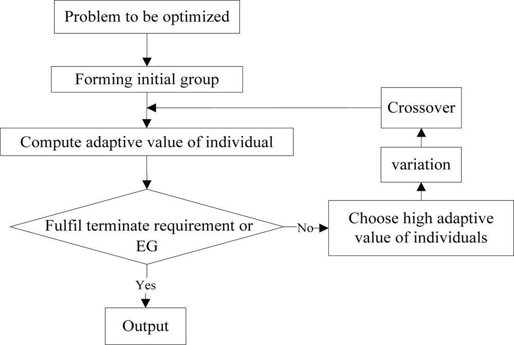
Compared with the traditional evolution algorithms, the DE retains the swarm-based global search strategy, uses real-coded, simple compilation operations based on differences and the survival strategy of one-to-one competition, and reduces the complexity of genetic manipulation. In addition the DE dynamically tracks current searches with its unique memory capability to adjust its search strategy. With its comparatively strong global convergence capability and robustness and no need with the help from information about the characteristics of problems, it is applicable for complex optimization problems [
19]. The basic flow is shown in
Figure 4.
In the DE, there are similar operations such as mutation in genetic algorithms, crossover and selection. Among them, the mutation operation is defined as [
18]:
where Pr
1 Pr
2 and Pr
3, are three different individuals randomly selected from evolution swarm, and F is a parameter between the interval [0.5, 1]. In (1), the parameter
F enlarges or shrinks the difference between two individuals, Pr
2 and Pr
3, randomly selected from the population swarm and adds them into the third individual Pr
1, and a new individual
C(
c1,
c2, ….,
cn). To increase the diversity of swarms, z crossover operation is introduced into the differential algorithm, and the specific operation is as the follows: for each piece value
xi of individuals Pr = (
x1,
x2,…,
xn) of the father generation, a random pi is generated at the interval [0, 1]. The big or small relationship between Pr and the parameter CR determines whether
xi is replaced with
ci in order to obtain a new individual Pr′ = (
x1′,
x2′,…,
xn′), in which xi′ = ci (when pi < CR) or xi (when pi ≥ CR). If the new individual Pr′ is better than the father-generation individual Pr, Pr will be replaced with Pr′. Otherwise it remains unchanged. In the differential evolution algorithm, selection operation uses the greedy strategy. Only when the generated offspring is better than father-generation individuals, the offspring will be retained. Otherwise, the father-generation individuals will be kept into the next generation.
4. LEACH Protocol Improvement Based on the Differential Evolution Algorithm
The LEACH protocol improvement based on the differential evolution algorithm executes in rounds the same as the traditional LEACH protocol. Each round execution is divided into four phases: (1) partitioning of initial clusters, (2) collecting status information about the nodes inside clusters by auxiliary cluster head nodes, (3) optimizing and selecting cluster heads with differential evolution algorithms, and (4) forming optimized clusters. Among them, the third one is the key to the improvements proposed in this paper, and will be described in detail.
4.1. Partitioning Initial Clusters
In this phase, the traditional LEACH routing algorithm is used for partitioning initial clusters for WSNs. The selection process of cluster head assignment by the LEACH protocol works as follows: each node creates a random number between 0∼1, and if the number is less than the threshold
T(
n), it sends a message to others that it is the cluster head. In each round of a cycle, if one node was a cluster head before, then
T(
n) is set to 0, so that node will not be elected again as a cluster head in this round. Non-elected nodes will be elected as cluster heads with probability
T(
n). The number of elected nodes increases, the threshold
T(
n) to elect the nodes from the remaining nodes increases, and the probability of the random number created by nodes less than
T(
n) increases, and the probability of nodes to become cluster heads increases correspondingly. When there is only one node that is not elected,
T(
n) = 1, which means the node must be elected as the cluster head.
T(
n) is given as:
where
P =
k/N is the percentage of cluster head accounted for all nodes, r is the number of election rounds, r mod (1/
P) refers to the number of nodes elected in the previous r-1 round of cycle, and G is a set of non-elected nodes in the previous r-1 round. It can be seen that the selection of cluster heads is determined by the elected times of nodes.
Nodes will broadcast ADV messages via the CSMA mechanism to all other ones to inform them that they became cluster heads when they compete successfully. The messages contain information such as IDs of cluster heads, etc. Non-cluster head nodes receive them, analyze and compare, find out the one with the strongest signal as its head cluster, and send a join-request message back to that cluster head, which contains the information of its own ID and that cluster head’s ID. When receiving it, that cluster head starts to create a TDMA schedule, uses the TDMA mechanism to allocate slots for each member in the cluster, and informs all nodes inside it. By now, the LEACH protocol has completed partitioning clusters. After that phase, cluster heads and clusters are basically determined, but blind nodes tend to appear in the clusters. Cluster heads in this phase is defined as auxiliary cluster heads.
4.3. Optimizing Algorithm and Determining Cluster Heads with the DE
The DE algorithm executes basically in the same way as other evolution algorithms, including coding, initial swarm formation, variation, crossover and selection operations. In order to make it suitable for the problem domain, the DE algorithm has to be modified, which is described in details as follows.
(1) Initial Swarm Formation: Initial swarms are formed with the corresponding groups of integer sequences of ID numbers of neighbor nodes the auxiliary cluster heads collect.
Defining the solution vector as:
Each solution vector is an evolution individual. Each generation of an evolution swarm is expressed as G, i, is an individual’s location in the swarm, n is the number of neighbor nodes auxiliary cluster heads collect, and NP is the scale of the swarm.
The first-generation swarm is created at random. The rule is to sort the IDs of neighbor nodes’ auxiliary cluster heads collected in an ascending order of
ID1 <
ID2 < …<
IDn, to create a corresponding relationship of
IDi ↔
i,
i = 1,…,
n, and to create the initial swarm based on that relationship. Each element in the swarm is given as:
where
rd is a random number between (0,1),
round [] is a closest integer, and
n is the number of neighbor nodes.
(2) Variation Operation: Variation Operation is an important step for the DE algorithm to create sub-individuals. The algorithm uses the variation mode of DE/rand/1 [
19]. Super-individuals, plus the difference between two or more individuals in the group create the sub-individuals. The basic unit of the variation operation is individual, which is solution vector.
For the evolution target vector of each generation
Xi,G,
i = 1,2,…,
NP, its variation operation is given by:
where
r1,
r2,
r3 are not equal random integers in [1,2,
NP], and not equal to
i. Xri,G is called the father individual or basic individual.
F is the variation factor, and
F ∈ (0,1).
(3) Crossover Operation: The crossover operation adds varieties to the swarm. It includes two modes, index crossover mode and binomial crossover mode. The algorithm uses the common binomial crossover mode defined as
where
randb(
j) is a random decimal figure between [0,1],
randr(
i) is a random integer between [1,
n] and
CR is the crossover factor.
(4) Selection Operation: In order to calculate the adaptation value of each experimental vector, it is necessary to establish an objective function first. Each vector is composed of n integers between 1∼n, corresponding to the ID numbers of the neighbor nodes, respectively. The purpose of establishing the function is to connect an actual physical relationship with abstract numbers in the algorithm to judge the quality of the vectors.
Determining the adaptation value of the experiment vectors not only needs to consider the energy of corresponding nodes, but also reflects the energy distribution of surrounding nodes. The further away from the node the neighbor nodes are, the greater the energy; and
vice versa. Based on this characteristic, an objective function is defined as:
where
α +
β = 1 and
α ∈ [0,1],
β ∈ [0,1];
ej is the energy of the corresponding node of element
j in the experiment vector (node
j in short);
ēj is the average energy of nodes except node
j; α is the influential energy factor of
ej; and
β is the influential energy factor of
ēj. Adjusting
α and
β will adjust the contribution rate of
ej and
ēj to the adaptation value. In this paper,
α =
β = 0.5.
The average equivalent energy
ēj is defined as:
where
ẽi =
f(
ei,
ri) is the equivalent energy of node
i. Suppose
ri is the distance from node
i to node
j, and
ei is the remaining energy of node
i. The remaining energy of node
i and its distance to node
j should be taken into account together for the structure of
f(
ei,ri). The following should be satisfied: the farther the distance from node
i to node
j, the less the equivalent energy of node
i, and
vice versa. The function reflects the characteristics of problems in simulation. In all, the target function is:
The experiment vector Ui,G+1 resulted from the crossover operation is compared with the objective vector Xi,G substituted into the vector objective function. If the objective function value of Ui,G+1 is greater than that of Xi,G, then Xi,G is replaced with Ui,G+1. And if not, Xi,G will be kept, thus the next generation swarm is created. By now, a swarm has finished a generation of evolution. The DE algorithm repeatedly executes the steps of variation, crossover and selection until the termination condition is satisfied. The termination condition is usually the evolution generations, and the element with the absolute dominant amount position in the experiment vectors is just the corresponding number of the final cluster head.
6. Conclusion
The ultimate goal of WSNs is to increase the sensing precision, accuracy of sensed information and to reduce redundant data of communications. The aim of precipitation monitoring, for example, is to improve the accuracy and real-time of precipitation data in the basin as well as to reduce the information loss of precipitation details. Existing hydrological stations must be built based on the conditions of good power supply, communications and transportation. The data from a single hydrographic station are often used to represent the precipitation information in its radius of a few hundred meters or even a few kilometers, and it would seriously affect the accuracy of regional precipitation information. WSNs for monitored environment avoid the dependence of monitor sites on the hydrological infrastructure, and geographical and terrain factors can be fully taken into account in the deployment of sensor nodes. The precipitation information collected via sensors can be representative for meteorological environment of the monitored region. In addition, the reduced cost of building stations and the reduced size of nodes make it possible to deploy more nodes. Based on requirements, the amount of precipitation information within the same area can be several, several hundred times or even higher than that of the existing hydrological station network. The decisions supported by that amount of information are much more accurate than by the traditional network.
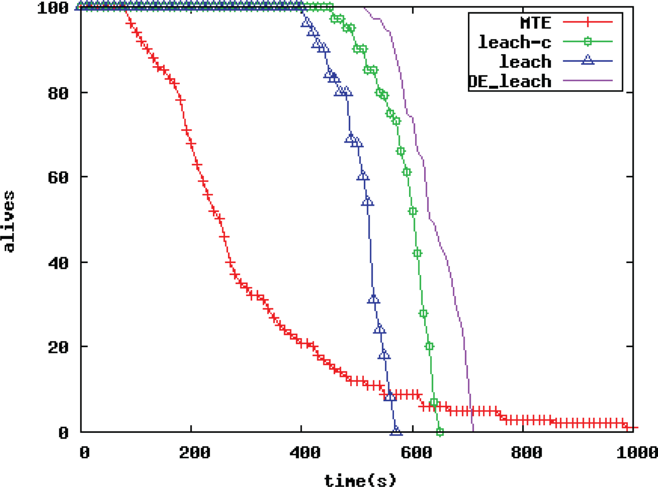
In wireless sensor networks, the performance of routing protocols determines the overall performance of the network, and the WSN routing protocols have always been a hot topic. This paper takes outdoor environmental monitoring applications such as meteorology and hydrology and wetland ecology field as the background. The paper proposes an improved LEACH routing algorithm based on the differential evolution algorithm (DE_LEACH routing algorithm) to address the shortcomings of the traditional LEACH routing protocol. The improved algorithm uses the simple and fast search features of the differential evolution algorithm (DE) to optimize multiple objectives for the selection process of cluster heads to improve energy efficiency and stability of the application system. The simulation results prove that the DE_LEACH routing algorithm proposed in this paper can effectively prevent blind nodes in normal clustering routing algorithms, improve the life cycle of large-scale WSNs as well as the quality, and make WSN routing protocols with the improvement in this paper more suitable for outdoor environmental monitoring applications such as meteorology and hydrology, wetland ecology field than other routing protocols.
The present research results are mainly on how to avoid an unreasonable distribution of cluster heads and how to prevent the emergence of blind nodes. Further studies will focus on how to improve the selection for each parameter to adaptively meet the needs of various applications in order to reduce the computing amount as much as possible.


