1. Introduction
With the development of the information society, there is higher and higher demand for communication systems. Therefore, how to transmit the information faster and better has become very important. Recently, high efficiency modulation technologies are receiving the attention by many researchers, especially Ultra Narrow Band (UNB) [
1,
2] communication with its outstanding transmission ability in the wireless communication field. The concept of UNB communication, first proposed by H. R. Walker, can obtain very high data rates and high spectra efficiency, even higher than traditional channel capacity. Consequently, many researchers begin to pay more attention to this “break” performance, and the extension to Shannon’s channel capacity equation has been proposed [
3].
In wireless sensor networks [
4], sensor nodes are typically powered by batteries with a limited lifetime, and even though energy-scavenging mechanisms can be adopted to recharge batteries through solar panels, piezo-electric or acoustic transducers, energy is still a limited resource and must be used judiciously, so efficient use of the sensor node battery’s energy is an important aspect of sensor networks. Therefore, many researchers have paid attention to this problem and proposed many energy management schemes [
5–
7].
During the research, we found that as a kind of UNB system, the Extended Binary Phase Shift Keying (EBPSK) [
8] modulation, proposed by Wu
et al., has better bandwidth efficiency [
9], high data rates, attractive energy efficiency [
10], and can greatly save energy for sensor nodes. However, the research on its BER performance just remains in the simulation stage and has no detailed theoretical derivations. So this paper will discuss this problem, which will provide the theoretical support for simulation results, and lay the foundation for the feasibility and rationality of UNB system.
The rest of this paper is organized as follows. In Section 2, a scheme for EBPSK- MODEM is introduced, of which the detailed derivation of BER performance is given, and also the SNR improvement performance is analyzed in Section 3. Then, Section 4 collects some simulation results, and conclusions are given in Section 5.
2. EBPSK Modulation and Demodulation
2.1. The Definition of EBPSK Modulation
EBPSK modulation [
8] is defined as follows:
where
g0(
t) and
g1(
t) is modulation waveform corresponding to bit “0” and bit “1”, respectively,
T is the bit duration,
τ is the phase modulation duration, and
θ is the modulating angle. Obviously, if
τ =
T and
θ =
π,
Eq.(1) degenerates to:
It is just the classical Binary Phase Shift Keying (BPSK) modulation, so is named as the Extended BPSK.
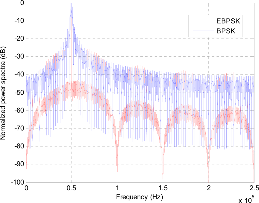
Figure 1 depicts the normalized the power spectral density (PSD) of the typical BPSK of
(2) and the EBPSK of
(1) at the same bit rate
R, where bit duration
T = 20
Tc = 20*2
π /
wc, the phase modulation duration
τ for EBPSK modulation lasts one period of carrier,
i.e.,
τ =
Tc = 2
π /
wc, the modulation angle
θ =
π, the amplitude
A = 1, and the carrier frequency
fc =
wc / 2
π = 50
KHz,
2.2. The Demodulation of EBPSK Signals
As we know, if
, the bit error ratio (BER) of the optimal BPSK receiver is calculated by:
where
Eb is the signal energy used for transmitting one bit, and
N0 is the
PSD of Addition Gaussian White Noise (AWGN).
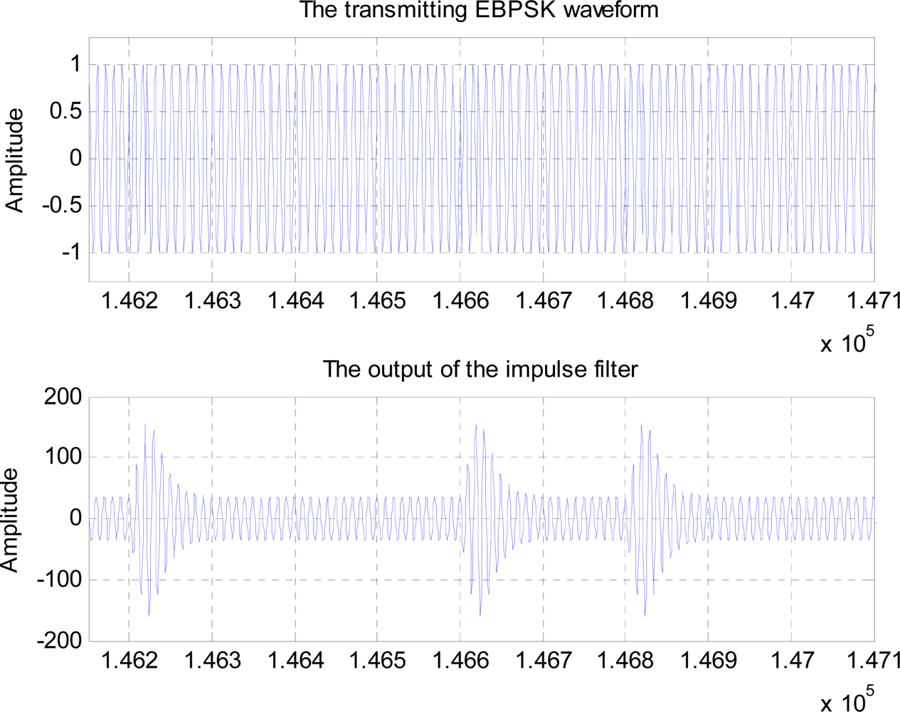
However, if the same optimal BPSK receiver using traditional matched filter was utilized as the EBPSK demodulator, the BER performance would be much poorer since the difference in EBPSK modulated waveforms corresponding to “0” and “1” is very tiny and hard to detect, although in
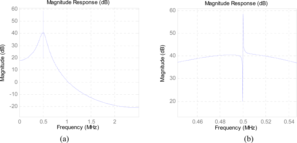
Figure 1 more centralized PSD of the EBPSK appears. Therefore a special infinite impulse response (IIR) filter as given in
Figure 2 is used in EBPSK receiver to produce high impulse at the phase jumping points
τ of bit 1s, so as to transform phase modulation into amplitude changes [
10]. And by this way it amplifies the signal characters as much as possible and removes utmost noise.
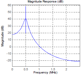
Figure 3 depicts the response of this filter to EBPSK modulated signals. Obviously, a simple amplitude detector followed would perform the demodulation of EBPSK signals because of the existence of high impulse in coded 1 s. Therefore, we gave this kind of filter the name of “impacting filter” [
10].
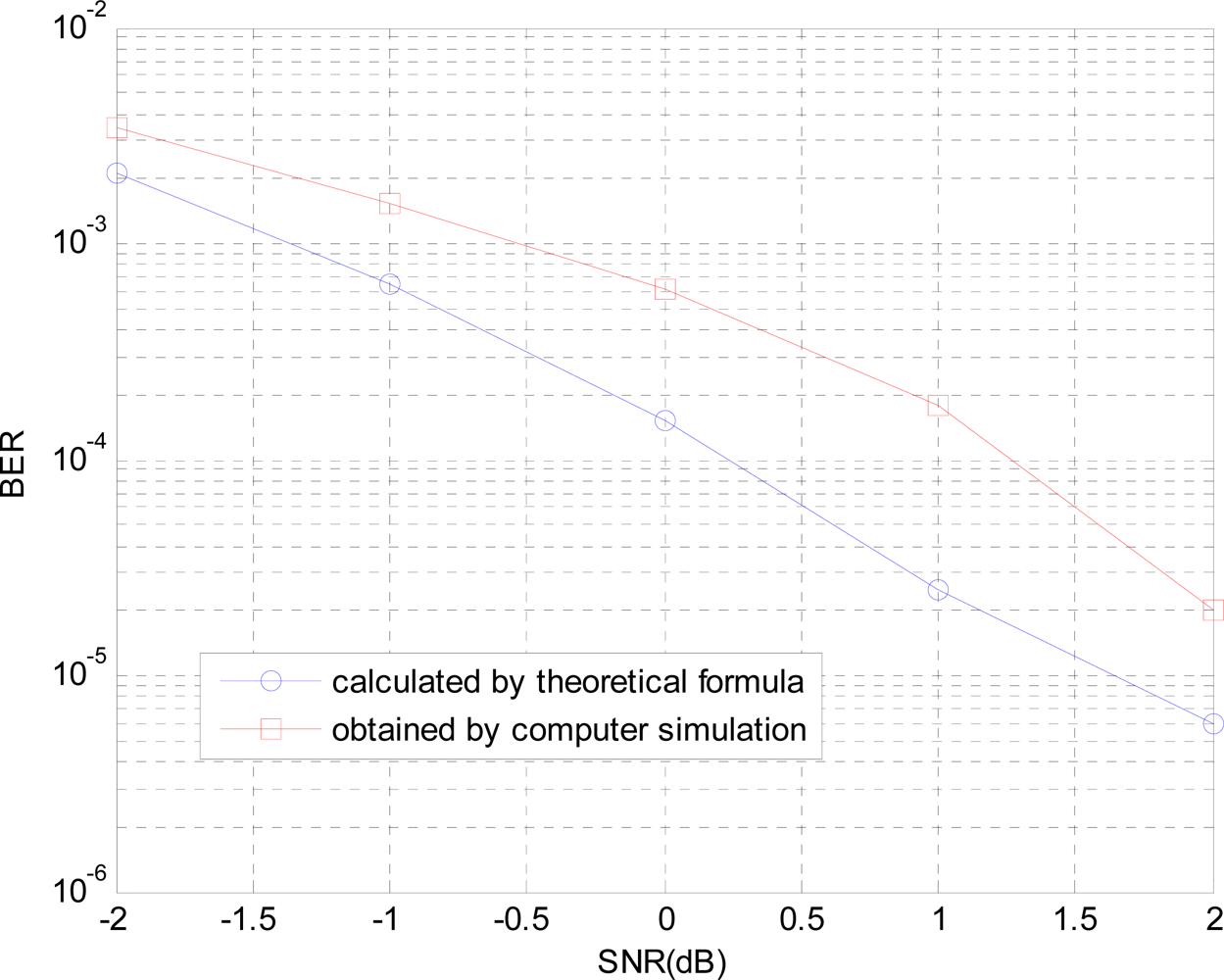
4. Simulation
In this section, in order to verify the correctness of theoretical analysis, we compare the BER results calculated by the theoretical formula with one obtained by computer simulation, as in
Figure 5, where system parameters in simulation are selected as:
fc = 930
KHz,
N = 20,
K = 2,
A =
B = 1, and
θ =
π. The paper chooses the receiver filter having three conjugate poles and one zero point, where the detail filter parameters is as ref. [
10].
According to the above results, the theoretical result and simulation result just have 1 dB difference in order to obtain the same BER performance, which is caused by the detection method and the choosing of the decision threshold in the simulation.
5. Discussion and Conclusions
(1) The
Pe−BPSK given in
(3) is an ideal and optimum value already, while the
Pe−EBPSK given in
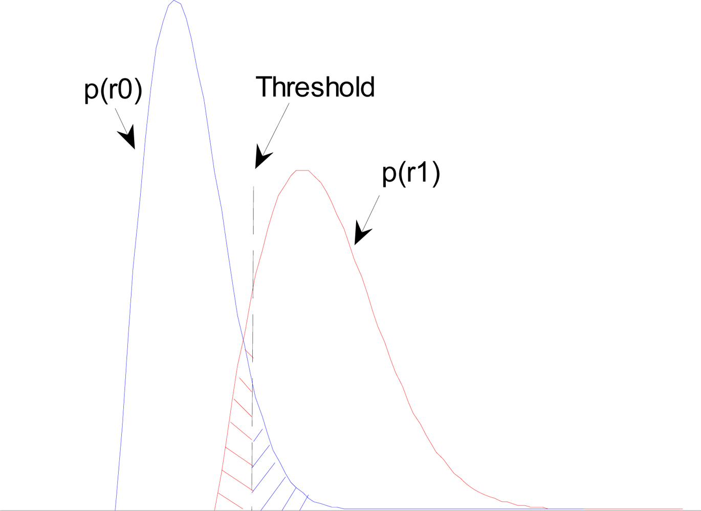
(7) is far from giving an optimal EBPSK receiver and still depends on the filter design. In other words, it leaves potential for EBPSK receivers to improve. For example, from the
Figure 4 we can imagine:
With the increasing of k, the peak distance of p(r0) and p(r1) becomes large, so the shaded area decreases, i.e., the minimum BER decreases.
With the decrease of σ2, although the peak distance of p(r0) and p(r1) remains unchanged, their shapes are narrowing, so the shaded area, or the minimum BER, decreases also.
Therefore, under certain conditions, the BER performance of the EBPSK modulation will outperform or be inferior to that of the BPSK modulation, and the spectral efficiency of the EBPSK system is much higher than BPSK.
(2) Substituting
k = 2 into
(21) we obtain an astonishing estimation as
SNR1 = 18
SNR0, which implies that as long as we can obtain larger value of
k by optimizing the impacting feature of the filter, the BER performance of the EBPSK system can be further improved.
To sum up, aimed at a UNB system, the EBPSK-MODEM, this paper has discussed the importance of the special impacting filter, deduced the BER formula of EBPSK system, analyzed the SNR improvement performance of impacting filter, discussed the choice of optimum decision threshold, and analyzed the reason or possibility for EBPSK to outperform BPSK both in spectral efficiency and in BER performance. Research on these special filters is underway, and a detailed introduction will be given in forthcoming papers.
Acknowledgments
The authors would like to thank the National Foundation of China (60872075), the Natural Science Foundation of Jiangsu Province (BK2007103), China Postdoctoral Science Foundation (20080441015), Jiangsu Planned Projects for Postdoctoral Research Funds (0802005B) and Southeast University Planned Projects for Postdoctoral Key Research Funds.
References and Notes
- Walker, H.R. Ultra Narrow Band Modulation Textbook. Available Online: http://www.vmsk.org/ (accessed on 23 July 2008).
- Wu, L.N. Advance in UNB high speed communications. Prog. Nat. Sci. (in Chinese) 2007, 17, 143–149. [Google Scholar]
- Feng, M.; Wu, L.N. Special non-linear filter and extension to Shannon's channel capacity. Digital Signal Proc. 2009, 19, 861–873. [Google Scholar]
- Akiyldiz, I.; Su, W.; Sankarasubramaniam, Y.; Cayirci, E. A survey on sensor networks. IEEE Commun. Mag. 2002, 40, 102–114. [Google Scholar]
- Suhinthan, M.; Saman, H; Malin, P. Energy efficient sensor scheduling with a mobile sink node for the target tracking application. Sensors 2009, 9, 696–716. [Google Scholar]
- Alippi, C.; Anastasi, G.; Di Francesco, M.; Roveri, M. An adaptive sampling algorithm for effective energy management in wireless sensor networks with energy-hungry sensors. IEEE Instrum. Meas. Mag. 2010, 59, 335–344. [Google Scholar]
- Anastasi, G.; Conti, M.; Francesco, M.; Passarella, A. Energy conservation in wireless sensor networks. Ad Hoc Netw 2009, 7, 537–568. [Google Scholar]
- Wu, L.N. UNB modulation in high speed space communications. Proc. SPIE 2007, 6795, 679510-1–679510-6. [Google Scholar]
- Feng, M.; Wu, L.N.; Qi, C.H. Analysis and optimization of power spectrum on EBPSK modulation in throughput-efficient wireless system. J. Southeast Univ 2008, 24, 143–148. [Google Scholar]
- Wu, L.N.; Feng, M.; Gao, P. An impulse filter method used in ABSK signal. Chinese Patent CN10029875.3,. 2009. [Google Scholar]
- Proakis, J.G. Digital Communications, 4th ed.; McGraw-Hill Book Company, Inc.: Columbus, OH, USA, 2001. [Google Scholar]
- Oppenheim, A.V.; Willsky, A.S. Signals and Systems, 2nd ed.; Publishing House of Electronics Industry: Beijing, China, 2009. [Google Scholar]
- Proakis, J.G.; Salehi, M. Communication System Engineering, 2nd ed.; Prentice Hall: Bergen County, NJ, USA, 2002. [Google Scholar]
© 2010 by the authors; licensee Molecular Diversity Preservation International, Basel, Switzerland. This article is an open-access article distributed under the terms and conditions of the Creative Commons Attribution license ( http://creativecommons.org/licenses/by/3.0/).
