Localization of Mobile Robots Using Odometry and an External Vision Sensor

Abstract
:
1. Introduction
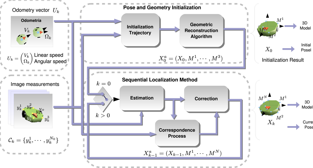
- Image measurements: they consist of the projection in the camera’s image plane of certain points of the robot’s 3D structure. The measurement process is in charge of searching coherent correspondences through images with different perspective changes due to the movement of the robot.
- Motion estimation of the robot: The odometry sensors built on-board the robot supply the localization system with an accurate motion estimation in short trajectories but that is prone to accumulative errors in large ones.
1.1. Previous Works
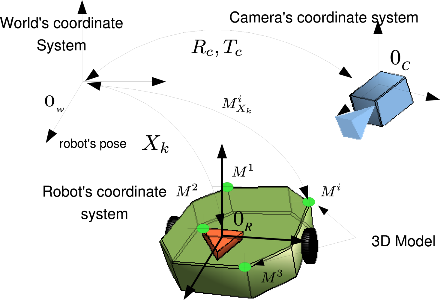
2. Definitions and Notation
2.1. Robot and Image Measurements
2.2. Random Processes
- Pose Xk = (X̂k, ∑k) and 3D model M = (M̂, ∑M) processes. Its joint distribution is encoded in .
- Measurement process Yk = (Ŷk, ∑Yk), whose uncertainty comes from errors in image detection.
- Odometry input values Uk = (Ûk, ∑Uk), which are polluted by random deviations.
3. Initialization Process
3.1. Odometry Estimation
3.2. Image Measurements
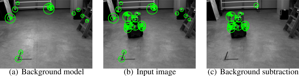
- Feature-based background subtraction.We describe the static background of the scene using a single image, from which a set of features, and its correspondent SIFT descriptors are obtained. The sets b and b are our feature-based background model.Given an input image, namely Ik, we find the sets k and k. We consider that a feature , belongs to the background if we can find a feature , such that and . This method although simple shows to be very effective and robust in real environments (See Figure 4).
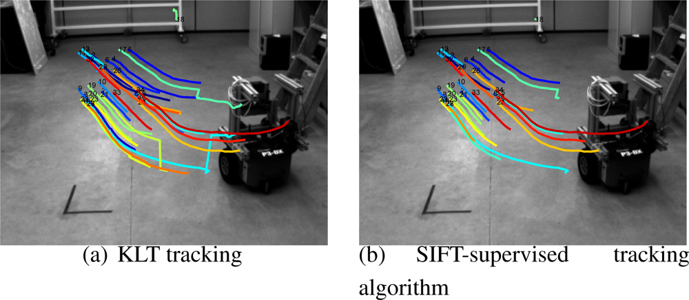
- Supervised tracking algorithm.Given the first image of the initialization trajectory, namely I1, we obtain the set of N features 1, once they are cleaned by the aforementioned background subtraction method. We propose a method to track them in the whole initialization trajectory.By only using SIFT descriptors and its tracking in consecutive frames does not produce stable tracks, specially when dealing with highly irregular objects where many of the features are due to corners. We thus propose to use a classical feature tracking approach based on the Kanade–Lucas–Tomasi (KLT) algorithm [14]. To avoid degeneracy in the tracks, which is a very common problem in those kind of trackers, we use the SIFT descriptors to remove those segments of the tracks that clearly do not correspond to the feature tracked. This can be done easily by checking distance between the descriptors in the track. The threshold used must be chosen experimentally so that it does not eliminate useful parts of the tracks. In Figure 5a we can see the tracks obtained by the KLT tracker without degeneracy supervision. In Figure 5b the automatically removed segments are displayed.
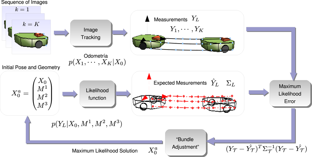
3.3. Likelihood Function
3.4. Maximum Likelihood Approach
3.5. Initialization before Optimization
3.6. Degenerate Configurations
- Straight motion: there is no information about the center of rotation of the robot and thus the pose has multiple solutions.
- Rotational motion around robot axis: the following one-parameter (i.e., n) family of solutions gives identical measurements in the image plane:with .
- Circular trajectory: under a purely circular trajectory the following one-parameter family of initialization vectors gives identical measurements in the image plane:
3.7. Obtaining the Gaussian Equivalent of the Solution
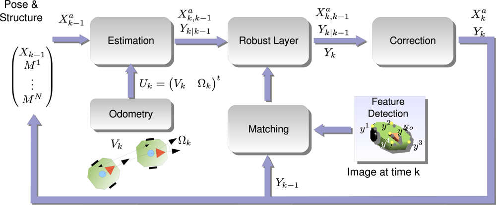
4. Online Robot Localization
- Estimation Step: using the previous pose distribution , defined by its mean and covariance matrix , and the motion model ga, a Gaussian distribution which infers the next state is given .
- Robust Layer: the correspondence between image measurements and the 3D model of the robot easily fails, so a number of wrongly correspondences or outliers pollute the measurement vector Yk. Using a robust algorithm and the information contained in the state vector, the outliers are discarded before the next step.
- Correction Step: using an outlier-free measurement vector, we are confident to use all the information available to obtain the target posterior distribution
4.1. Estimation Step
4.2. Correction Step
4.3. Robust Layer
4.4. Image Measurements
5. Results
5.1. Simulated Data
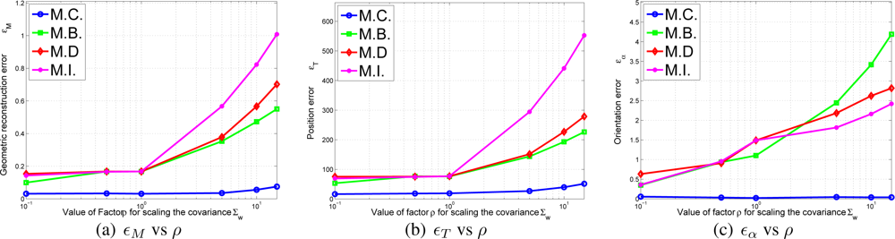
- Initialization errors in function of the odometry error. In this experiment the value of and are multiplied by the following multiplicative factor:The different errors of Equation 43 can be viewed in Figure 9a–c in terms of ρ. As it can be observed in the results, the M.C. (Complete correlated matrix ∑L) method outperforms the rest of approximations of ∑L, specially the full diagonal method M.I., which means that the statistical modelling proposed in this paper is effective.
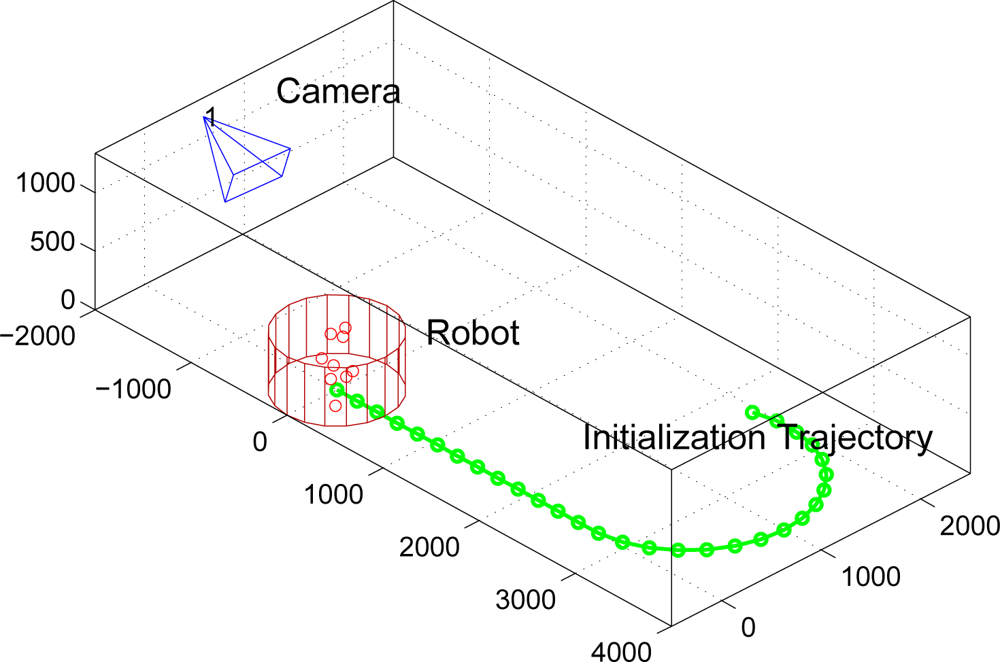
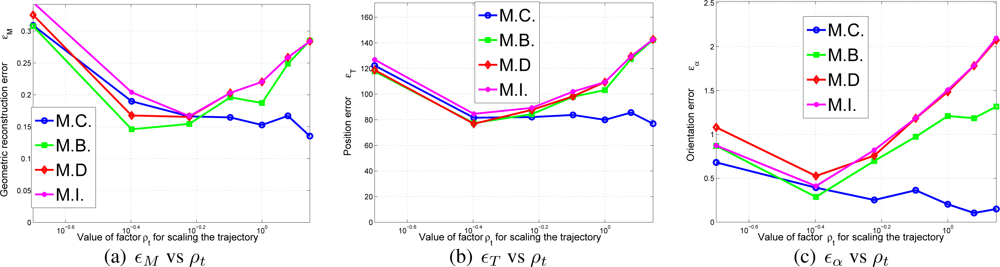
- Initialization errors in function of the trajectory length. The trajectory used in the experiment and displayed in Figure 8 is uniformly scaled by parameter ρt,so that it can be guessed the relationship between trajectory length and initialization errors. In Figure 10 the initialization errors are displayed versus ρt.In light of the results shown in Figure 10a–c, the M.C. method is capable of reducing the error no matter how large is the trajectory chosen. However, in the rest of the approximations of ∑L there is an optimal point where the initialization errors are minimum. This results make sense, as without statistical modelling large trajectories contain accumulative errors which usually affects the final solution of .
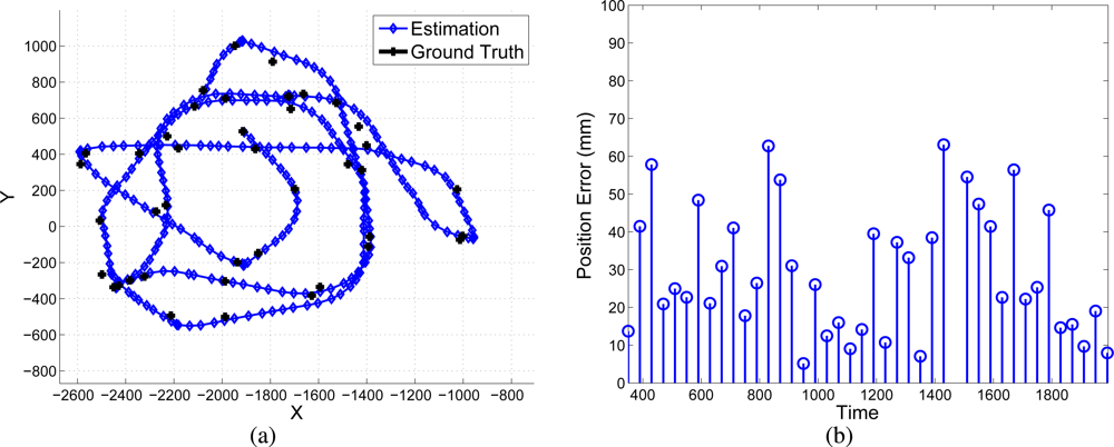
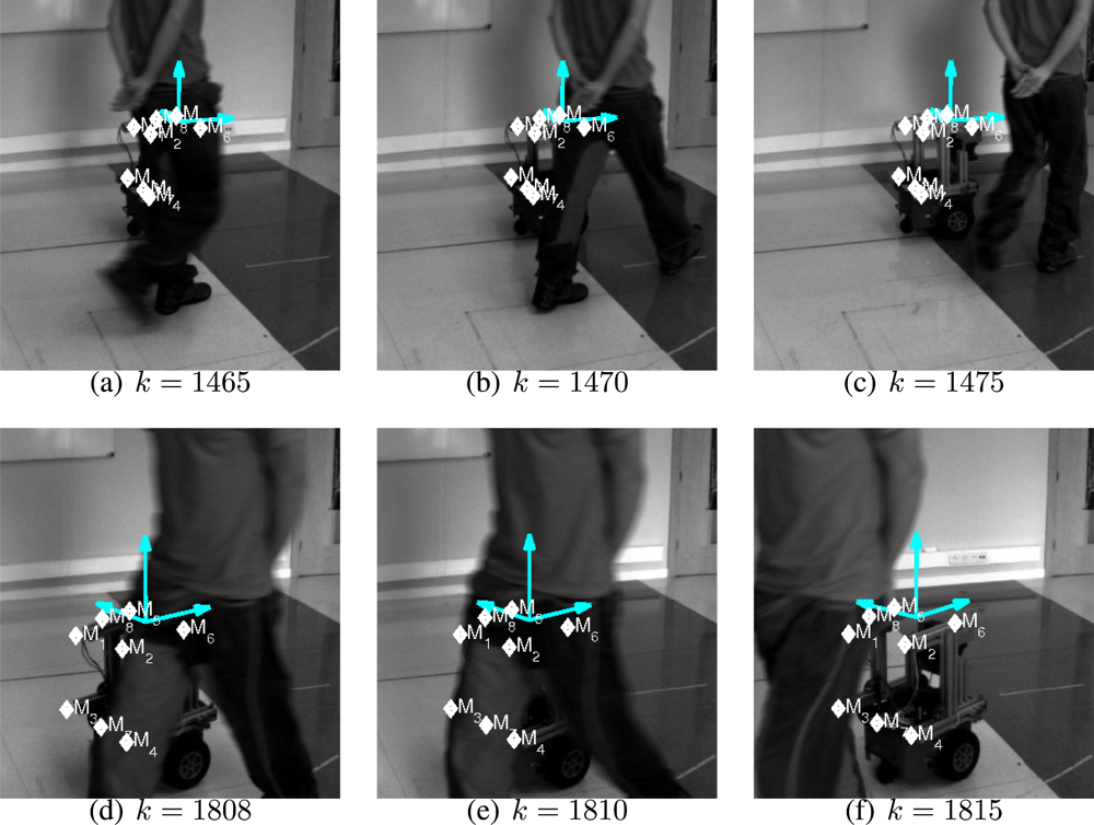
5.2. Real Data
6. Conclusions
- The initialization step provides a non-supervised method for obtaining the initial pose and structure of the robot previously to its sequential localization. A Maximum Likelihood cost function is proposed, which obtains the pose and geometry given a trajectory performed by the robot. The proposal of this paper allows to compensate for the odometry drift in the solution. Also an exact initialization method has been proposed and the degenerate configurations have been identified theoretically.
- The online approach of the algorithm obtains the robot’s pose by using a sequential Bayesian inference approach. A robust step, based on the RANSAC algorithm, is proposed to clean the measurement vector out of outliers.
- The results show that the proposed method is suitable to be used in real environments. The accuracy and non-drifting nature of the pose estimation have been also evaluated in a real environment.
Acknowledgments
References
- Lee, J.; Hashimoto, H. Intelligent space concept and contents. Advanced Robotics 2002, 16, 265–280. [Google Scholar]
- Aicon 3D. Available online: www.aicon.de (accessed January 2010).
- ViconPeak. Available Online: www.vicon.com (accessed January 2010).
- Se, S.; Lowe, D.; Little, J. Vision-based global localization and mapping for mobile robots. IEEE Trans. Robotics Automat 2005, 21, 364–375. [Google Scholar]
- Davison, A.J.; Murray, D.W. Simultaneous Localization and Map-Building Using Active Vision. IEEE Trans. Patt. Anal 2002, 24, 865–880. [Google Scholar]
- Hada, Y.; Hemeldan, E.; Takase, K.; Gakuhari, H. Trajectory tracking control of a nonholonomic mobile robot using iGPS and odometry. Proceedings of IEEE International Conference on Multisensor Fusion and Integration for Intelligent Systems, Tokyo, Japan; 2003; pp. 51–57. [Google Scholar]
- Fernandez, I.; Mazo, M.; Lazaro, J.; Pizarro, D.; Santiso, E.; Martin, P.; Losada, C. Guidance of a mobile robot using an array of static cameras located in the environment. Auton. Robots 2007, 23, 305–324. [Google Scholar]
- Morioka, K.; Mao, X.; Hashimoto, H. Global color model based object matching in the multi-camera environment. Proceedings of IEEE /RSJ International Conference on Intelligent Robots and Systems, Beijing, China; 2006; pp. 2644–2649. [Google Scholar]
- Chung, J.; Kim, N.; Kim, J.; Park, C.M. POSTRACK: a low cost real-time motion tracking system for VR application. Proceedings of Seventh International Conference on Virtual Systems and Multimedia, Berkeley, CA, USA; 2001; pp. 383–392. [Google Scholar]
- Sogo, T.; Ishiguro, H.; Ishida, T. Acquisition of qualitative spatial representation by visual observation. Proceedings of International Joint Conference on Artificial Intelligence, Stockholm, Sweden; 1999. [Google Scholar]
- Kruse, E.; Wahl, F.M. Camera-based observation of obstacle motions to derive statistical data for mobile robot motion planning. Proceedings of IEEE International Conference on Robotics and Automation, Leuven, Belgium; 1998; pp. 662–667. [Google Scholar]
- Hoover, A.; Olsen, B.D. Sensor network perception for mobile robotics. Proceedings of IEEE International Conference on Robotics and Automation, Krakow, Poland; 2000; pp. 342–347. [Google Scholar]
- Steinhaus, P.; Ehrenmann, M.; Dillmann, R. MEPHISTO. A Modular and extensible path planning system using observation. Lect. Notes Comput. Sci 1999, 1542, 361–375. [Google Scholar]
- Shi, J.; Tomasi, C. Good features to track. Proceedings of IEEE Conference on Computer Vision and Pattern Recognition, Seattle, WA, USA; 1994; pp. 593–600. [Google Scholar]
- Lowe, D.G. Distinctive image features from scale-invariant keypoints. Int. J. Comput. Vision 2004, 60, 91–110. [Google Scholar]
- Triggs, B.; McLauchlan, P.; Hartley, R.; Fitzgibbon, A. Bundle adjustment–a modern synthesis. Lect. Notes Comput. Sci 1999, 1883, 298–372. [Google Scholar]
- Hartley, R.; Zisserman, A. Multiple View Geometry in Computer Vision, 2nd ed.; Cambridge University Press: Cambridge, UK, 2003. [Google Scholar]
- Moreno-Noguer, F.; Lepetit, V.; Fua, P. Accurate non-iterative o (n) solution to the PnP problem. Proceedings of IEEE International Conference on Computer Vision, Rio de Janeiro, Brasil; 2007; pp. 1–8. [Google Scholar]
- Schweighofer, G.; Pinz, A. Globally optimal o (n) solution to the pnp problem for general camera models. Proceedings of BMVC, Leeds, UK; 2008. [Google Scholar]
- Van der Merwe, R.; de Freitas, N.; Doucet, A.; Wan, E. The Unscented Particle Filter; Technical Report CUED/F-INFENG/TR380; Engineering Department of Cambridge University: Cambridge, UK, 2000. [Google Scholar]
- Pizarro, D.; Mazo, M.; Santiso, E.; Hashimoto, H. Mobile robot geometry initialization from single camera. Field and Service Robotics; Springer Tracts in Advanced Robotics: Heidelberg, Germany, 2008; pp. 93–102. [Google Scholar]
- Fischler, M.A.; Bolles, R.C. Random sample consensus: a paradigm for model fitting with applications to image analysis and automated cartography. Comm. Assoc. Comp. Match 1981, 24, 381–395. [Google Scholar]
- GEINTRA. Group of Electronic Engineering Applied to Intelligent Spaces and Transport. Available online: http://www.geintra-uah.org/en (accessed December 2009).
- Bouguet, J.Y. Matlab Calibration Toolbox. Available online: http://www.vision.caltech.edu/bouguetj/calib-doc (accessed December 2008).


| Type of Approximation | cost function |
|---|---|
| Complete Correlated matrix ∑L (M.C.) | |
| 2N × 2N block approximation of ∑L (M.B.) | |
| 2 × 2 block approximation of ∑L (M.D.) | |
| Identity approximation of ∑L (M.I.) |
© 2010 by the authors; licensee Molecular Diversity Preservation International, Basel, Switzerland. This article is an open-access article distributed under the terms and conditions of the Creative Commons Attribution license http://creativecommons.org/licenses/by/3.0/.
Share and Cite
Pizarro, D.; Mazo, M.; Santiso, E.; Marron, M.; Jimenez, D.; Cobreces, S.; Losada, C. Localization of Mobile Robots Using Odometry and an External Vision Sensor. Sensors 2010, 10, 3655-3680. https://doi.org/10.3390/s100403655
Pizarro D, Mazo M, Santiso E, Marron M, Jimenez D, Cobreces S, Losada C. Localization of Mobile Robots Using Odometry and an External Vision Sensor. Sensors. 2010; 10(4):3655-3680. https://doi.org/10.3390/s100403655
Chicago/Turabian StylePizarro, Daniel, Manuel Mazo, Enrique Santiso, Marta Marron, David Jimenez, Santiago Cobreces, and Cristina Losada. 2010. "Localization of Mobile Robots Using Odometry and an External Vision Sensor" Sensors 10, no. 4: 3655-3680. https://doi.org/10.3390/s100403655