Fiber Bragg Grating Sensor for Fault Detection in Radial and Network Transmission Lines

Abstract
:
1. Introduction
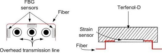
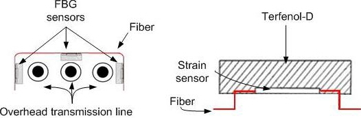
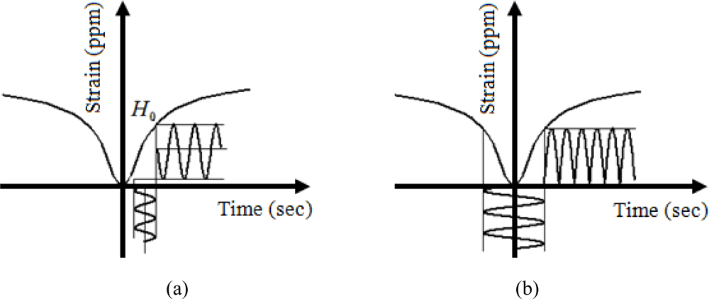
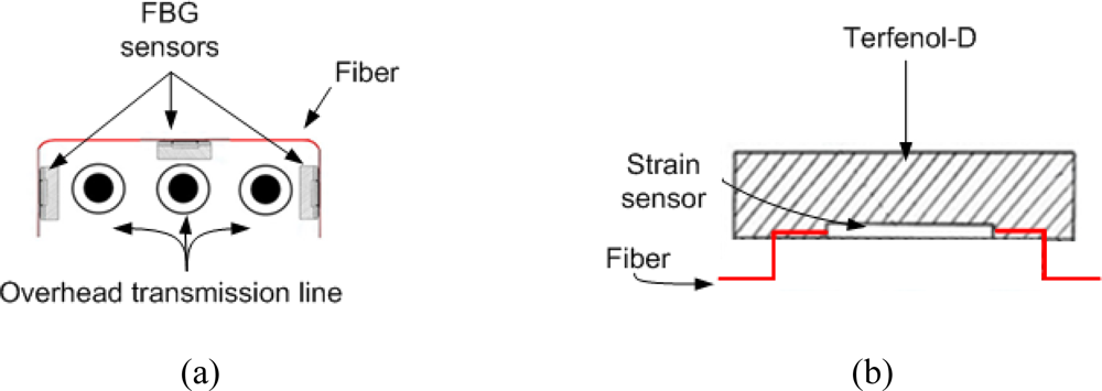
2. Magnetostrictive Materials
3. FBG Sensors
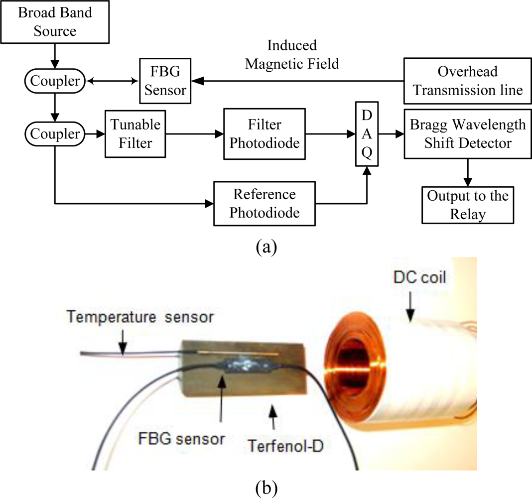
4. Development of the Concept
5. Simulation Result
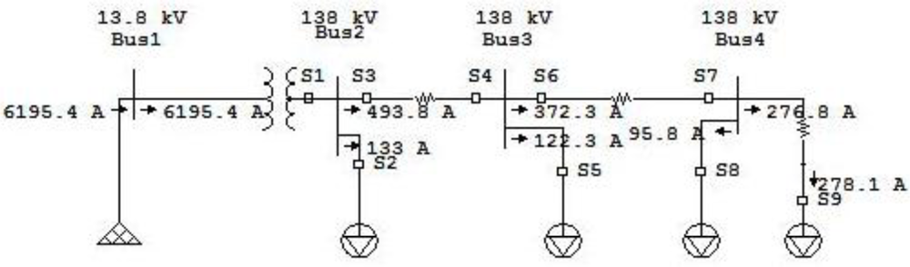
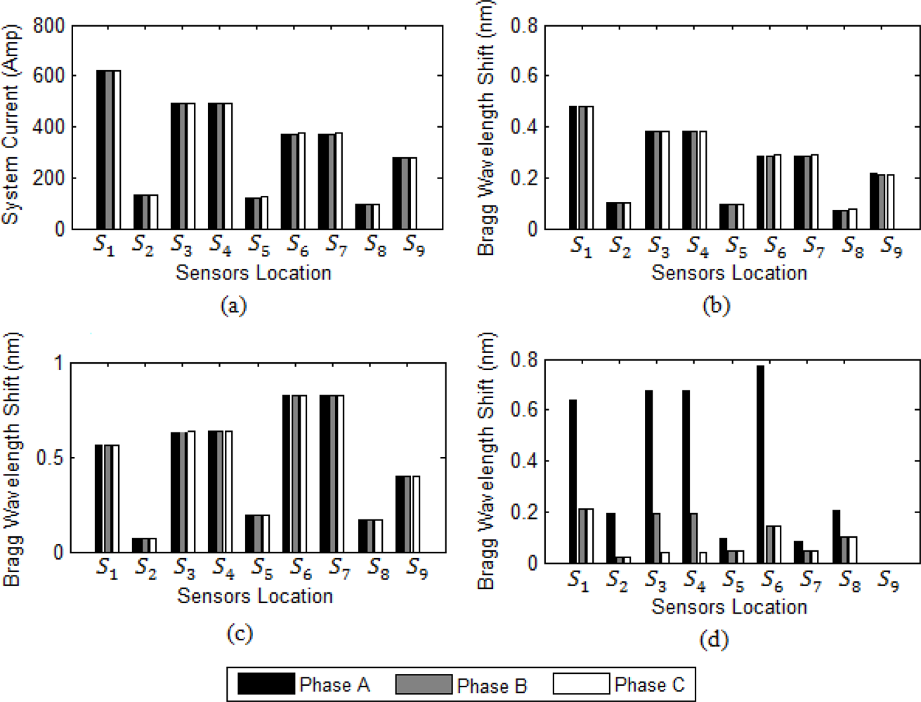
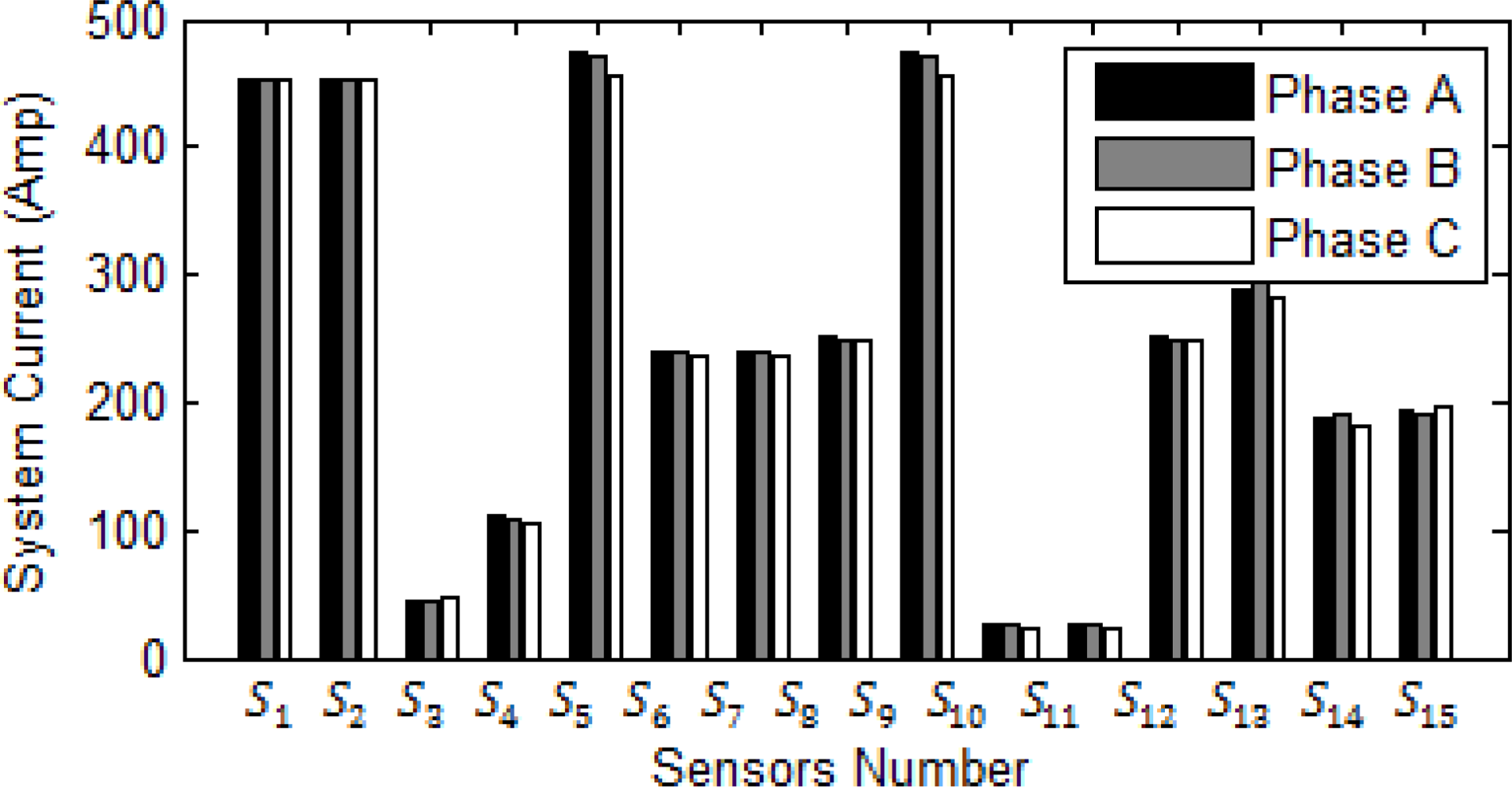
5.1. Radial System
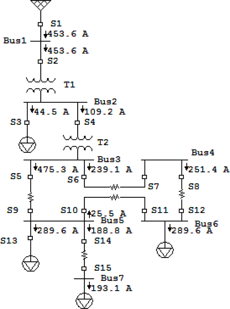
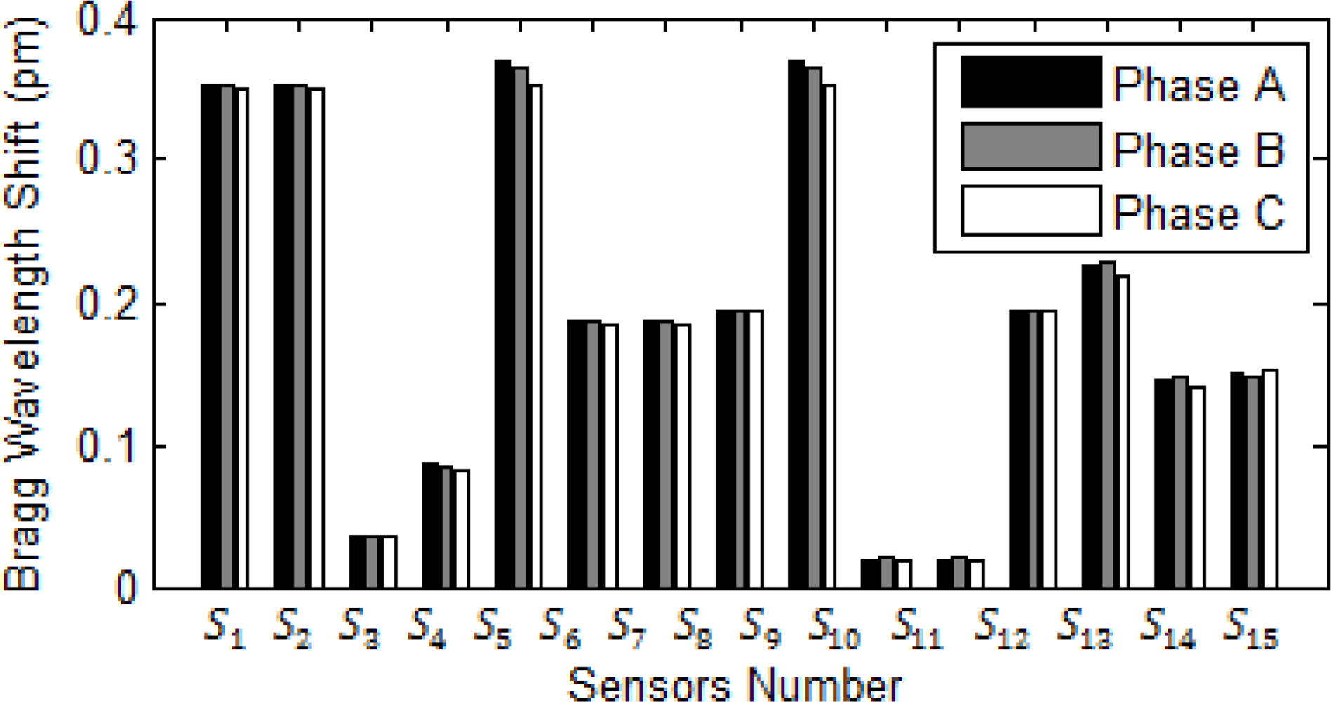
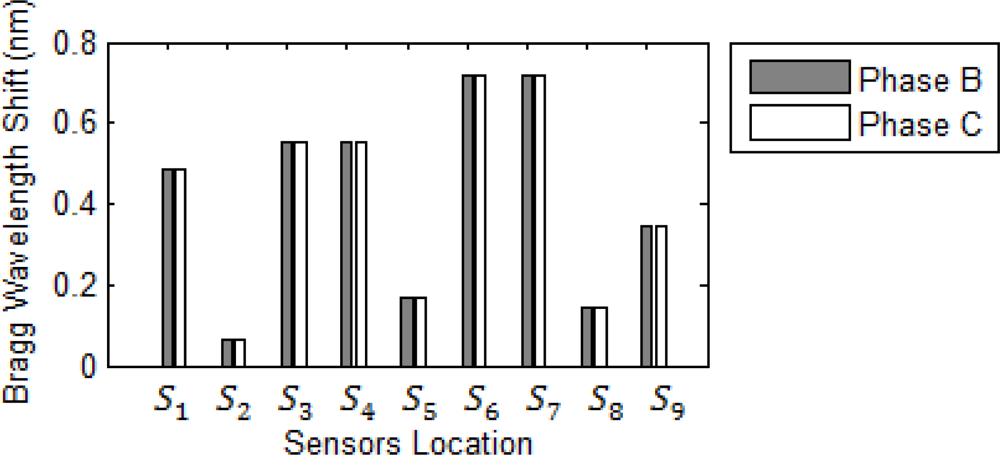
5.2. Network System
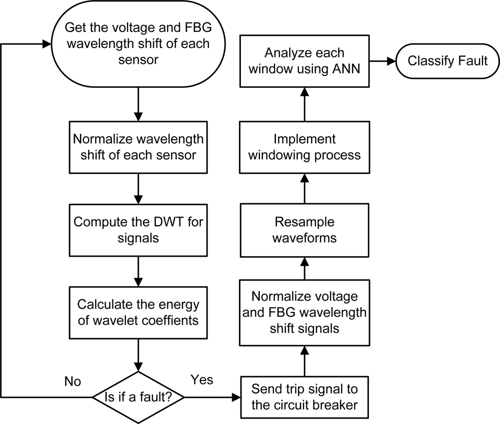
5.3. Fault detection and Classification Algorithm
- If Δλpos ≈ Δλpre, it is not a fault.
- If Emax < E*, it is not a fault.
- If Emax ≥ E*and Δλpos ≤ 0.14Δλpre, it is not a fault.
- If Emax ≥ E*and|Δλpos − Δλpre| < 0.14 max{Δλpos, Δλpre} it is not a fault.
- If Emax ≥ E*, and none of aforementioned rules have not met, it is a fault.
4. Conclusions
References
- Kucuksari, S; Karady, G. Experimental comparison of conventional and optical current transformers. IEEE Trans. Power Delivery 2010, 25, 2455–2463. [Google Scholar]
- Gang, Z; Shaohui, L; Zhipeng, Z; Wei, C. A novel electro-optic hybrid current measurement instrument for high-voltage power lines. IEEE Trans Instru Meas 2001, 50. [Google Scholar]
- Bohnert, K; Gabus, P; Nehring, J; Brandle, H. Temperature and Vibration Insensitive Fiber-Optic Current Sensor. J. Lightwave Tech 2002, 20, 267–276. [Google Scholar]
- Rochford, KB; Rose, AH; Day, GW. Magneto-optic sensors based on iron garnets. IEEE Trans. Mag 1996, 32, 4113–4117. [Google Scholar]
- Law, CT; Bhattarai, K; Yu, DC. Fiber-optics-based fault detection in power systems. IEEE Trans. Power Delivery 2008, 23, 1271–1279. [Google Scholar]
- Li, Y; Li, W; Han, X; Li, J. Application of multi-sensor information fusion technology in the power transformer fault diagnosis. Proceedings of International Conference on Machine Learning and Cybernetics, Boading, China, July 2009; pp. 29–33.
- Orr, P; Niewczas, P; Dysko, A; Booth, C. FBG-based fiber-optic current sensors for power systems protection: Laboratory evaluation. the Proceedings of the 44th International Universities Power Engineering Conference (UPEC), Leuven, Belgium, May 2009; pp. 1–5.
- Engdahl, G. Handbook of Giant Magnetostrictive Materials; Academic: New York, NY, USA, 2000. [Google Scholar]
- Calkins, F; Dapino, M; Flatau, AM. Effect of prestress on the dynamic performance of a terfenol-D transducer. Presented at the SPIE Symposium Smart Structures and Materials, San Diege, CA, USA; 1997. [Google Scholar]
- Sun, L; Zheng, Z. Numerical simulation on coupling behavior of Terfenol-D rods. Int. J. Solids Struct 2006, 43, 1613–1623. [Google Scholar]
- Groom, NJ; Bloodgood, VD. A comparison of analytical & experimental data for a magnetic actuator; NASA/TM 200-210328; NASA Langley Research Center Hampton: VA, 23681–2199; September 2000; pp. 1–16. [Google Scholar]
- Claeyssen, F; Lhermet, N; Le Letty, R; Bouchilloux, P. Actuators, transducers and motors based on giant magnetostrictive materials. J. Alloys Compounds 1997, 258, 61–73. [Google Scholar]
- Tan, X; Baras, JS. Modeling and control of hysteresis in magnetostrictive actuators. J. Automatica 2004, 40, 1469–1480. [Google Scholar]
- Dapino, MJ; Smith, RC; Flatau, AB. Structural magnetic strain model for magnetostrictive transducers. IEEE Trans. Mag 2000, 36, 545–556. [Google Scholar]
- Kashyap, R. Fiber Bragg Grating; Academic Press: Burlington, MA, USA, November 2009. [Google Scholar]
- Dziuda, L; Fusiek, G; Niewczas, P; Burt, GM; McDonald, JR. Laboratory evaluation of the hybrid fiber-optic current sensor. J. Sens. Actuat. A: Phys 2007, 136, 184–190. [Google Scholar]
- Or, SW; Nersessian, N; Carman, GP. Dynamic magnetomechanical behavior of terfenol-D/Epoxy 1-3 particulate composites. IEEE Trans. Mag 2004, 40, 71–77. [Google Scholar]
- Karunanidhi, S; Singaperumal, M. Design, analysis and simulation of magnetostrictive actuator and its application to high dynamic servo valve. J. Sensor. Actuat. A Phys 2010, 157, 185–197. [Google Scholar]
- Zhao, H; Xiong, YL; Zhang, J; Wang, SR. Measurement of power frequency AC current using FBG and GMM. IEEE ISEIM Int. Symp. Elect. Insulat. Mater 2005, 3, 741–743. [Google Scholar]
- Mora, J; Diez, A; Cruz, JL; Andres, MV. A Magnetostrictive sensor interrogated by fiber gratings for DC-Current and temperature discrimination. IEEE Photonics Tech Lett 2000, 12, 1680–1682. [Google Scholar]
- Moghadas, A; Barnes, R; Shadaram, M. An innovative fiber bragg grating sensor capable of fault detection in radial power systems. Proceeding of 4th Annual IEEE Systems Conference, San Diego, CA, USA, March 2010; pp. 165–168.
- Moghadas, A; Shadaram, M. Novel fiber bragg grating sensor applicable for fault detection in high voltage transformers. Proceedings of IEEE Conference on Innovative Technologies for an Efficient and Reliable Electric Supply, Waltham, MA, USA, September 2010.
- Reilly, D; Willshire, AJ; Fusiek, G; Niewczas, P; McDonald, JR. A fiber bragg grating based sensor for simultaneous AC current and temperature measurement. IEEE Sensors J 2006, 6, 1539–1542. [Google Scholar]
- Melle, S; Liu, K; Measures, R. A Passive demodulation system for guided wave bragg grating sensors. IEEE Photonics Tech. Lett 1992, 4, 516–518. [Google Scholar]
- Jiang, JA; Fan, PL; Cen, CS; Yu, C; Sheu, JY. A fault detection and faulted-phase selection approach for transmission lines with haar wavelet transformers. Proceeding IEEE/PES Transmission and Distribution Conference and Exhibition, Dallas, TX, USA, September 7–12, 2003; pp. 285–289.
- Vasilic, S; Kezunovic, M. Fuzzy art neural network algorithm for classifying the power system faults. IEEE Trans. Power Delivery 2005, 20, 1306–1314. [Google Scholar]
- Silva, KM; Souza, BA; Brito, NSD. Fault detection and classification in transmission lines based on wavelet transform and ANN. IEEE Trans. Power Delivery 2006, 21, 2058–2063. [Google Scholar]
- Hong, YY; Chang-Chian, PC. detection and correction of distorted current transformer current using wavelet transform and artificial intelligence, generation, transmission & distribution. IET 2008, 2, 566–575. [Google Scholar]
- Haykin, S. Neural Networks: A Comprehensive Foundation, 2nd ed; Prentice-Hall: Upper Saddle River, NJ, USA, July 1999. [Google Scholar]
- Daubechies, I. Ten Lectures on Wavelets. Proceedings of CBMS-NSF Regional Conference Series in Applied Mathematics, Philadelphia, PA, USA; 1992. [Google Scholar]


| Fault type | Phase A (output 1) | Phase B (output 2) | Phase C (output 3) | Ground (output 4) |
|---|---|---|---|---|
| AG | 1 | 0 | 0 | 1 |
| BG | 0 | 1 | 0 | 1 |
| CG | 0 | 0 | 1 | 1 |
| AB | 1 | 1 | 0 | 0 |
| AC | 1 | 0 | 1 | 0 |
| BC | 0 | 1 | 1 | 0 |
| ABG | 1 | 1 | 0 | 1 |
| ACG | 1 | 0 | 1 | 1 |
| BCG | 0 | 1 | 1 | 1 |
| ABC | 1 | 1 | 1 | 0 |
| No Fault | 0 | 0 | 0 | 0 |
| Variables | Training | Validation | Test |
|---|---|---|---|
| Fault location (km) | 10-30-50-70-90 100-120-140 | 60–110 | 80–130 |
| Fault type | AG-BG-CG-AB-BC-AC-ABG-BCG-ACG-ABC | ||
| Fault resistance (Ω) | Phase-Phase: 0.5 and 5 Phase-Ground: 10, 50 and 100 | ||
| Real system change | Expected change in system | Number of iterations | Number of Success |
|---|---|---|---|
| Voltage sag | No fault | 45 | 45 |
| Line de-energization | No fault | 70 | 70 |
| Normal operation | No fault | 25 | 25 |
| AG fault | AG fault | 70 | 70 |
| AB fault | AB fault | 70 | 68 |
| ABG fault | ABG fault | 70 | 68 |
| ABC fault | ABC fault | 70 | 70 |
| 420 | 416 | ||
| Real system change | Expected change in system | Number of iterations | Number of Success |
|---|---|---|---|
| Voltage sag | No fault | 45 | 45 |
| Line de-energization | No fault | 70 | 70 |
| Normal operation | No fault | 25 | 25 |
| AG fault | AG fault | 70 | 69 |
| AB fault | AB fault | 70 | 67 |
| ABG fault | ABG fault | 70 | 67 |
| ABC fault | ABC fault | 70 | 70 |
| 420 | 413 | ||
© 2010 by the authors; licensee MDPI, Basel, Switzerland. This article is an open access article distributed under the terms and conditions of the Creative Commons Attribution license (http://creativecommons.org/licenses/by/3.0/).
Share and Cite
Moghadas, A.A.; Shadaram, M. Fiber Bragg Grating Sensor for Fault Detection in Radial and Network Transmission Lines. Sensors 2010, 10, 9407-9423. https://doi.org/10.3390/s101009407
Moghadas AA, Shadaram M. Fiber Bragg Grating Sensor for Fault Detection in Radial and Network Transmission Lines. Sensors. 2010; 10(10):9407-9423. https://doi.org/10.3390/s101009407
Chicago/Turabian StyleMoghadas, Amin A., and Mehdi Shadaram. 2010. "Fiber Bragg Grating Sensor for Fault Detection in Radial and Network Transmission Lines" Sensors 10, no. 10: 9407-9423. https://doi.org/10.3390/s101009407