Electro‐Quasistatic Analysis of an Electrostatic Induction Micromotor Using the Cell Method

Abstract
:
1. Introduction
2. Finite Formulation for the Micromotor
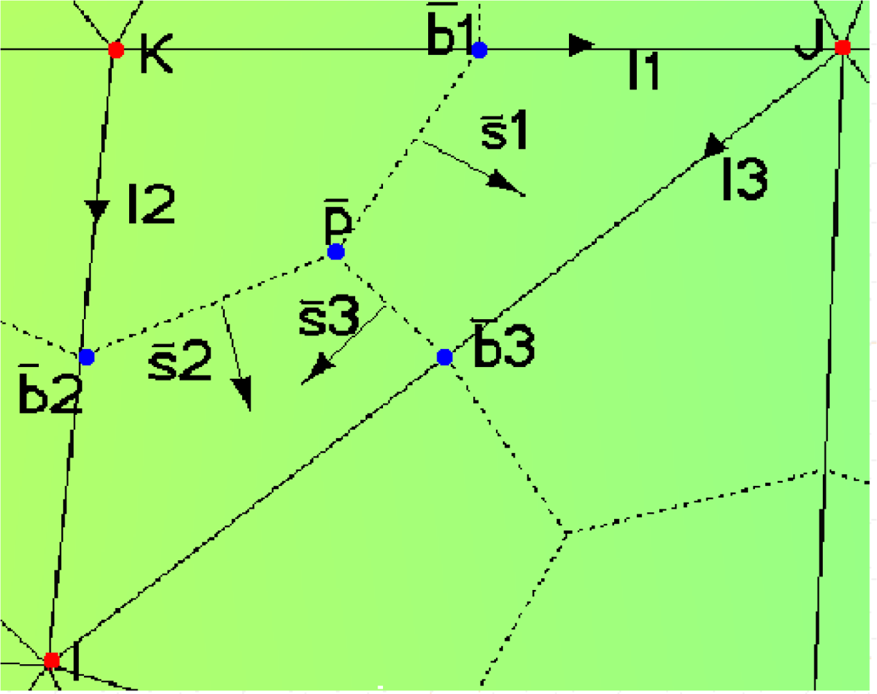
2.1. Topological Equation of the Micromotor in Discrete Form
2.2. Constitutive Equation of the Micromotor in Discrete Form
2.3. Final Global Equation of the Micromotor
3. Results
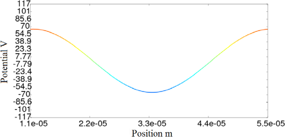
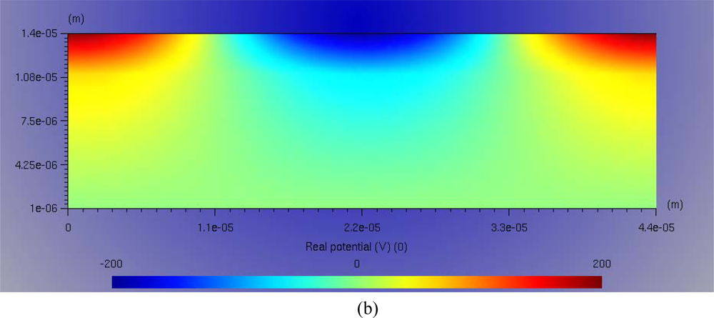
3.1. Discrete Field in Frequency Domain
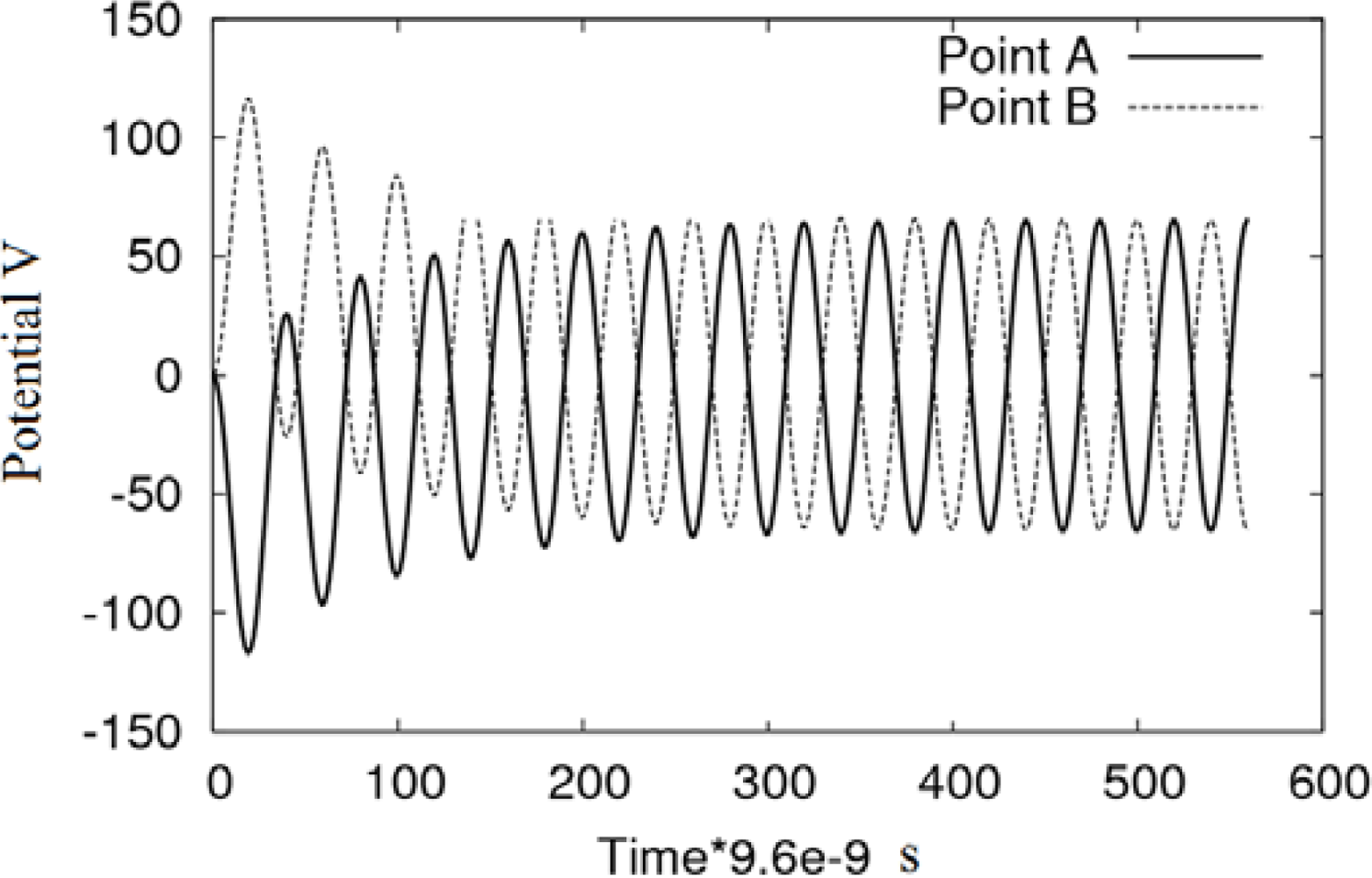
3.1. Discrete Field in Time Domain
4. Conclusions
References
- Tonti, E. On the geometrical structure of the electromagnetism. In Gravitation, Electromagnetism and Geometrical Structures, for the 80th Birthday; Lichnerowicz, A, Ferrarese, G, Eds.; Pitagora Editrice: Bologna, Italy, 1995; pp. 281–308. [Google Scholar]
- Tonti, E. A direct discrete formulation for the wave equation. J. Comp. Acoust 2001, 9, 1355–1382. [Google Scholar]
- Tonti, E. Finite formulation of the electromagnetic field. Int. Compumag Soc. Newslett 2001, 8, 5–11. [Google Scholar]
- Tonti, E. A direct discrete formulation of field laws: The cell method. Comput. Model. Eng. Sci 2001, 2, 237–258. [Google Scholar]
- Marrone, M. Computational aspects of the cell method in electrodynamics. J. Electromagn. Wave. Applicat 2001, 15, 407–408. [Google Scholar]
- Alotto, P; Perugia, I. Matrix properties of a vector potential cell method for magnetostatics. IEEE Trans. Magn 2004, 40, 1045–1048. [Google Scholar]
- Livermore, C; Forte, AR; Lyszczarz, T; Umans, SD; Ayon, AA; Lang, JH. A high–power MEMS electric induction motor. J. Microelectromech. Syst 2004, 13, 465–471. [Google Scholar]
- Irudayaraj, SS; Emadi, A. Micromachines: Principles of Operation, Dynamics, and Control. Proceedings of 2005 IEEE Int. Electric Machines and Drives Conference, San Antonio, TX, USA, May 2005; pp. 1108–1115.
- Neugebauer, TC; Perreault, DJ; Lang, JH; Livermore, C. A six–phase multilevel inverter for MEMS electrostatic induction machines. IEEE Trans. Circuit. Syst. II 2004, 51, 49–56. [Google Scholar]
- Santana, FJ; Monzón, JM; García–Alonso, S; Montiel–Nelson, JA. Analysis and modeling of an electrostatic induction micromotor. Proceedings of IEEE International Conference on Electrical Machines, Villamoura, Portugal, September 2008.
- Clemens, M; Weiland, T. Discrete electromagnetism with the finite integration technique. Prog Electromagn Res 2001, Pier 32. 65–87. [Google Scholar]
- Bettini, P; Trevisan, F. Electrostatic analysis for plane problems with finite formulation. IEEE Trans. Magn 2003, 39, 1127–1130. [Google Scholar]
- Bullo, M; Dughiero, F; Guarnieri, M; Tittonel, E. Isotropic and anisotropic electrostatic field computation by means of the cell method. IEEE Trans. Magn 2004, 20, 1013–1016. [Google Scholar]
- Clemens, M. Large Systems of equations in a discrete electromagnetism: formulations and numerical algorithms. IEE Proc. Sci. Meas. Technol 2005, 152, 50–57. [Google Scholar]
- Steinmetz, T; Helias, M; Wimmer, G; Fichte, LO; Clemens, M. Electro–quasistatic field simulations based on a discrete electromagnetism formulation. IEEE Trans. Magn 2006, 42, 755–758. [Google Scholar]
- Nagle, SF; Livermore, C; Frechette, LG; Ghodssi, R; Lang, JH. An electric induction micromotor. IEEE J. Microelectromech. Syst 2005, 14, 1127–1143. [Google Scholar]
- Marrone, M. Properties of constitutive matrices for electrostatic and magnetostatic problems. IEEE Trans. Magn 2004, 40, 1516–1520. [Google Scholar]
- Dular, P; Specogna, R; Trevisan, F. Coupling between circuits and A–x discrete geometric approach. IEEE Trans. Magn 2006, 42, 1043–1046. [Google Scholar]
- Schreiber, U; Clemens, M; van Rienen, U. Conformal FIT formulation for simulations of electro-quasistatic fields. Int. J. Appl. Electromagn. Mech 2004, 19, 193–197. [Google Scholar]
- Dular, P; Specogna, R; Trevisan, F. Constitutive matrices using hexahedra in a discrete approach for eddy currents. IEEE Trans. Magn 2008, 44, 694–697. [Google Scholar]
- Steinmetz, T; Wimmer, G; Clemens, M. Numerical simulation of transient electro-quasistatic fields using advanced subspace projection techniques. Adv. Radio Sci 2006, 4, 49–53. [Google Scholar]
- Steinmetz, T; Wimmer, G; Clemens, M. Adaptive linear-implicit time integration using subspace projection techniques for electroquasistatic and thermodynamic field simulations. IEEE Trans. Magn 2007, 43, 1273–1276. [Google Scholar]
- Steinmetz, T; Wimmer, G; Clemens, M. Acceleration of linear–implicit time integration schemes using subspace projection techniques for electro-quasistatic field simulations. Proceedings of 12th Biennial IEEE Conference on Electromagnetic Field Computation, Miami, FL, USA, April 2006.
- Nicolet, A; Delince, F. Implicit Runge–Kutta methods for transient magnetic field computation. IEEE Trans. Magn 1996, 32, 1405–1408. [Google Scholar]
- Wang, H; Taylor, S; Simkin, J; Biddlecombe, C; Trowbridge, B. An adaptative-step time integration method applied to transient magnetic field problems. IEEE Trans. Magn 2001, 37, 3478–3481. [Google Scholar]


| Symbol | Name | Unity |
|---|---|---|
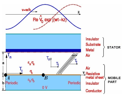
| a | Height of the air gap | m |
| b | Height of insulator | m |
| k | Number of waves per metre | - |
| l | Length | m |
| j | Imaginary unity | - |
| Jf | Current density | A/m2 |
| S | Slip | - |
| t | Thickness | m |
| ν | Linear speed of mobile part | m/s |
| V | Interelectrodic potential | V |
| V0 | Supply potential | V |
| εa | Electric permittivity of the air | F/m |
| εb | Electric permittivity of the insulator | F/m |
| εeff | Effective permittivity | F/m |
| φ | Electric scalar potential | V |
| ω | Angular frequency of the signal | Hz |
| σa | Electric conductivity of the air | S/m |
| σb | Electric conductivity of the insulator | S/m |
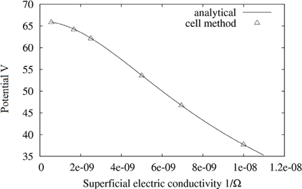
| σS | Superficial electric conductivity | 1/Ω |
| σeff | Effective Conductivity | S/m |
| Φb | Potential at the interface | V |
| Symbol | Name | Value | Unit |
|---|---|---|---|
| L | Length of the structure | 44 | μm |
| hm | Height of the metal sheet | 0.01 | μm |
| a | Height of dielectric 2 | 3 | μm |
| b | Height of dielectric 1 | 10 | μm |
| k | Number of waves per meter | 2π/L | μm−1 |
| ν | Linear speed of mobile part | 0 | μm/s |
| f | Temporal frequency of excitation | 2.6 × 10⁶ | Hz |
| V0 | Maximum value of excitation | 200 | V |
| Conductivity 1/Ω | Analytical solution V | CM V | Error % |
|---|---|---|---|
| 1/(50·106) | 21.6688 | 21.6947 | −0.119 |
| 1/(100·106) | 37.7909 | 37.7259 | 0.172 |
| 1/(200·106) | 53.6311 | 53.5904 | 0.075 |
| 1/(600·106) | 64.2738 | 64.2748 | −0.001 |
| 1/(1800·106) | 65.8906 | 65.9102 | −0.029 |
| Conductivity 1/Ω | Analytical solution V/m | CM V/m | Error % |
|---|---|---|---|
| 1/(50·106) | 3094307 | 3102000 | −0.248 |
| 1/(100·106) | 5381641 | 5389700 | −0.149 |
| 1/(200·106) | 7658503 | 7665400 | −0.090 |
| 1/(600·106) | 9178278 | 9182800 | −0.049 |
| 1/(1800·106) | 9409100 | 9419900 | −0.114 |
| Number of nodes | Number of elements | Analytical solution V | CM V | Error % |
|---|---|---|---|---|
| 2353 | 4704 | 65.89 | 65.91 | 0.030 |
| 613 | 1224 | 65.89 | 66.02 | 0.197 |
| 284 | 566 | 65.89 | 66.20 | 0.470 |
| 170 | 338 | 65.89 | 66.40 | 0.774 |
© 2010 by the authors; licensee MDPI, Basel, Switzerland. This article is an open access article distributed under the terms and conditions of the Creative Commons Attribution license (http://creativecommons.org/licenses/by/3.0/).
Share and Cite
Monzón-Verona, J.M.; Santana-Martín, F.J.; García–Alonso, S.; Montiel-Nelson, J.A. Electro‐Quasistatic Analysis of an Electrostatic Induction Micromotor Using the Cell Method. Sensors 2010, 10, 9102-9117. https://doi.org/10.3390/s101009102
Monzón-Verona JM, Santana-Martín FJ, García–Alonso S, Montiel-Nelson JA. Electro‐Quasistatic Analysis of an Electrostatic Induction Micromotor Using the Cell Method. Sensors. 2010; 10(10):9102-9117. https://doi.org/10.3390/s101009102
Chicago/Turabian StyleMonzón-Verona, José Miguel, Francisco Jorge Santana-Martín, Santiago García–Alonso, and Juan Antonio Montiel-Nelson. 2010. "Electro‐Quasistatic Analysis of an Electrostatic Induction Micromotor Using the Cell Method" Sensors 10, no. 10: 9102-9117. https://doi.org/10.3390/s101009102