1. Introduction
Protein structures are stabilized by several non-covalent interactions, such as hydrophobic, van der Waals, electrostatic, and hydrogen bonding interactions [
1,
2]. Of all the interactions that take place in proteins, hydrophobic interaction is a dominant force that drives protein folding. The interaction between non-polar amino-acid residues and the aqueous environment provides a strong hydrophobic force for protein folding [
1,
3], forming a hydrophobic core in the protein interior. Thus, the variation in hydrophobicity from the hydrophobic core to hydrophilic exterior is the spatial variation for most globular proteins. To quantify the spatial transition of hydrophobicity between the interior and the surface of globular proteins of known structure, Silverman [
4] introduced the second-order hydrophobic moment, using the hydrophobicity consensus scale of Eisenberg [
5]. The second-order hydrophobic moment, or quadrupole moment, is similar to the electrostatic quadrupole, and it was first proposed by Eisenberg [
5] to describe the hydrophobic distributions of proteins. A second-order hydrophobic moment has also been applied to the systems [
6] including native and decoy protein structures, and multi-domain proteins [
7]. In contrast, the first-order hydrophobic moment, or hydrophobic dipole moment, is similar to the dipole moment of a molecule. The first-order hydrophobic moment has been used to measure the amphiphilicity of primary and secondary structures either in globular proteins [
5,
8–
10] or in transmembrane proteins [
11,
12]. Moreover, the zeroth-order hydrophobic moment is the total hydrophobicity of the amino-acid residues in a protein, and it is similar to a net molecular charge.
Residues classified as buried or exposed are conventionally described by a geometric parameter calculated using the solvent-accessible surface area (ASA) [
13], which is generated by rolling a spherical probe with a radius of 1.4 Å over the surface of a protein. The ASA values obtained are in absolute values, and these can be changed to relative values, which are also known as the percentage of solvent accessibility
p (%) [
14,
15]. These values have been calculated using the ASA value of each amino-acid residue in the native state normalized with respect to the ASA value of the corresponding residue X in the extended state either of Gly-X-Gly [
16,
17] or of Ala-X-Ala [
14,
15]. Recently, the prediction of solvent accessibility, based on protein sequences, has also been developed using support vector regression (SVR) [
18–
21]. Gromiha
et al. [
14,
15] have classified these relative values to the locations of protein residues as follows: 0–2% as completely buried, 2–20% as a location between buried and partially buried, 20–50% as partially buried, and greater than 50% as completely exposed. This classification is used to study the stability changes for protein mutants.
Silverman [
4] used an ellipsoidal representation for the shapes of proteins. The extent of an ellipsoid was defined by a distance,
d, which was calculated from the molecular moments of geometry [
4]. The second-order hydrophobic moment per residue in a protein was calculated from a small value of
d to a larger value by increasing the value of
d until all residues in the protein have been collected to obtain its spatial distribution of the second-order hydrophobic moment. In contrast, the percentage of solvent accessibility,
p (%), is adopted in this work, and we employ successive increases of solvent accessibility; that is, increases from 0 to 100% are used to study the spatial distributions of the second-order hydrophobic moment of the protein structures. The second-order hydrophobic moment per residue is calculated from a space defined by a small value of
p (%), which collected the residues at the hydrophobic core of a protein to the larger value of
p (%) at which all residues will be collected. To investigate spatial characteristics, the distances from the origin of a protein to the centroids of the protein residues in a space defined by
p (%) are also considered. Here, we use the center of mass of each protein as the origin. In this work, two sets of hydrophobic parameters for each of the amino-acid residues in the protein structures are used in a comparative study of the second-order hydrophobic moments: one is based on the hydrophobicity consensus scale of Eisenberg [
5], and the other is derived from the partial atomic charges assigned to atoms of a protein in the CHARMM program [
22].
In this work, a different approach from the works of Silverman [
4] is used to define the spaces in a protein;
i.e., we employ
p (%) to define the spaces to calculate the spatial distributions of the second-order hydrophobic moment of a protein. The purpose of this study is to examine whether the hydrophobicity of each residue in a protein can be obtained using molecular modeling, and whether the values of hydrophobicity derived from the partial atomic charges assigned to atoms of a protein in the CHARMM program [
22] are comparable with those of the consensus scale of Eisenberg [
5] by using the spatial distributions of the second-order hydrophobic moment in the new definition of spaces in the protein. This work may provide an alternative way to calculate the hydrophobicity of each residue in a protein. Since the hydrophobicity of an amino-acid residue cannot be defined and measured easily, it is usually obtained from the free energy changes calculated by transferring amino-acid side chains from aqueous to non-aqueous media [
23,
24] or from non-aqueous to aqueous media [
25].
2. Materials and Methods
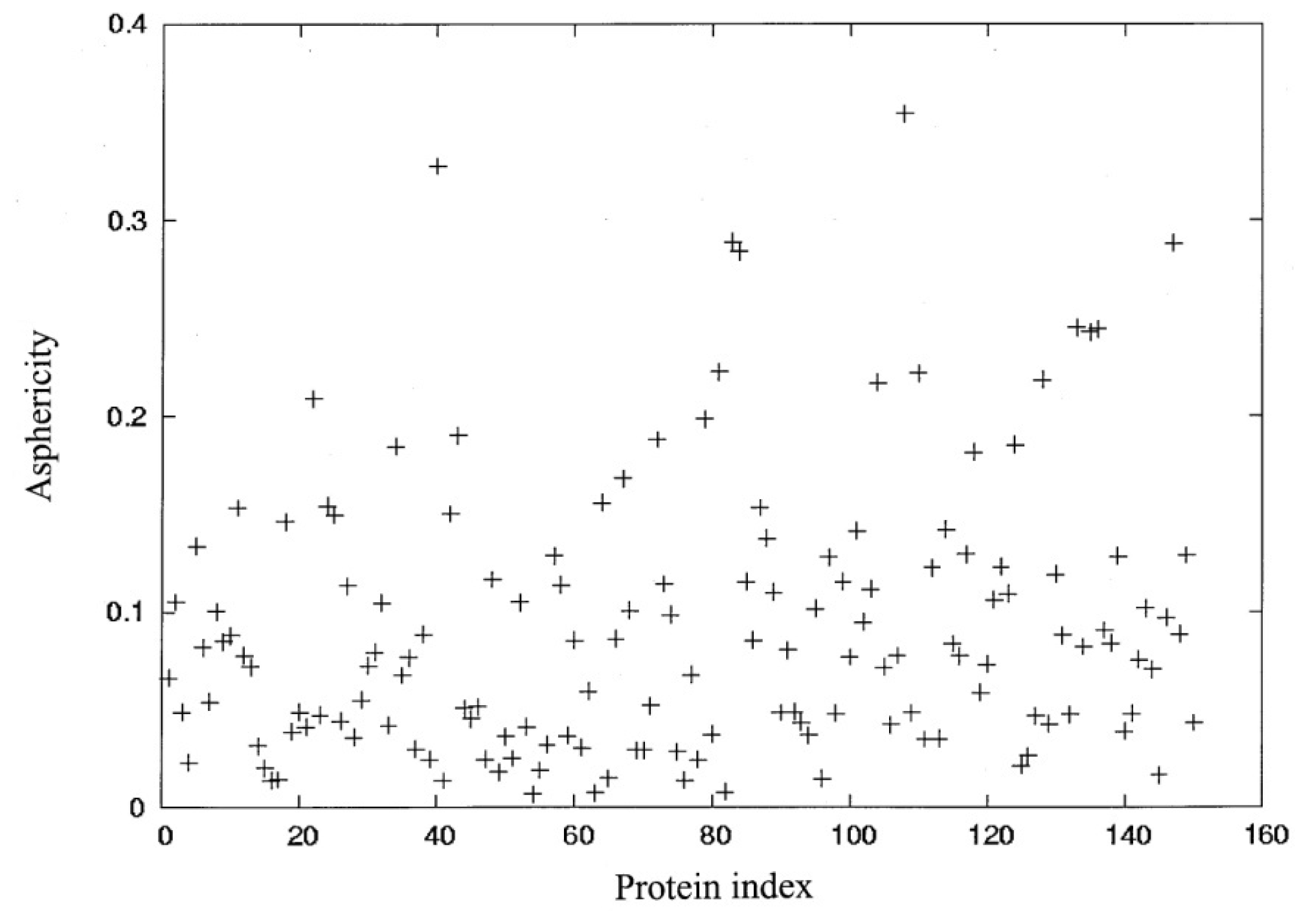
A set of 150 nonhomologous protein chains was randomly selected from PDBSELECT [
26], which included more than 4,000 protein chains. The sequence identity in this set of proteins is lower than 25%, and their single-chain protein crystal structures have been determined at a resolution of less than 1.8Å and at an R-factor of less than 0.18. All the structures of the proteins were obtained from the PDB [
27]. A figure of asphericity (
δ) and the index of 150 proteins are shown in
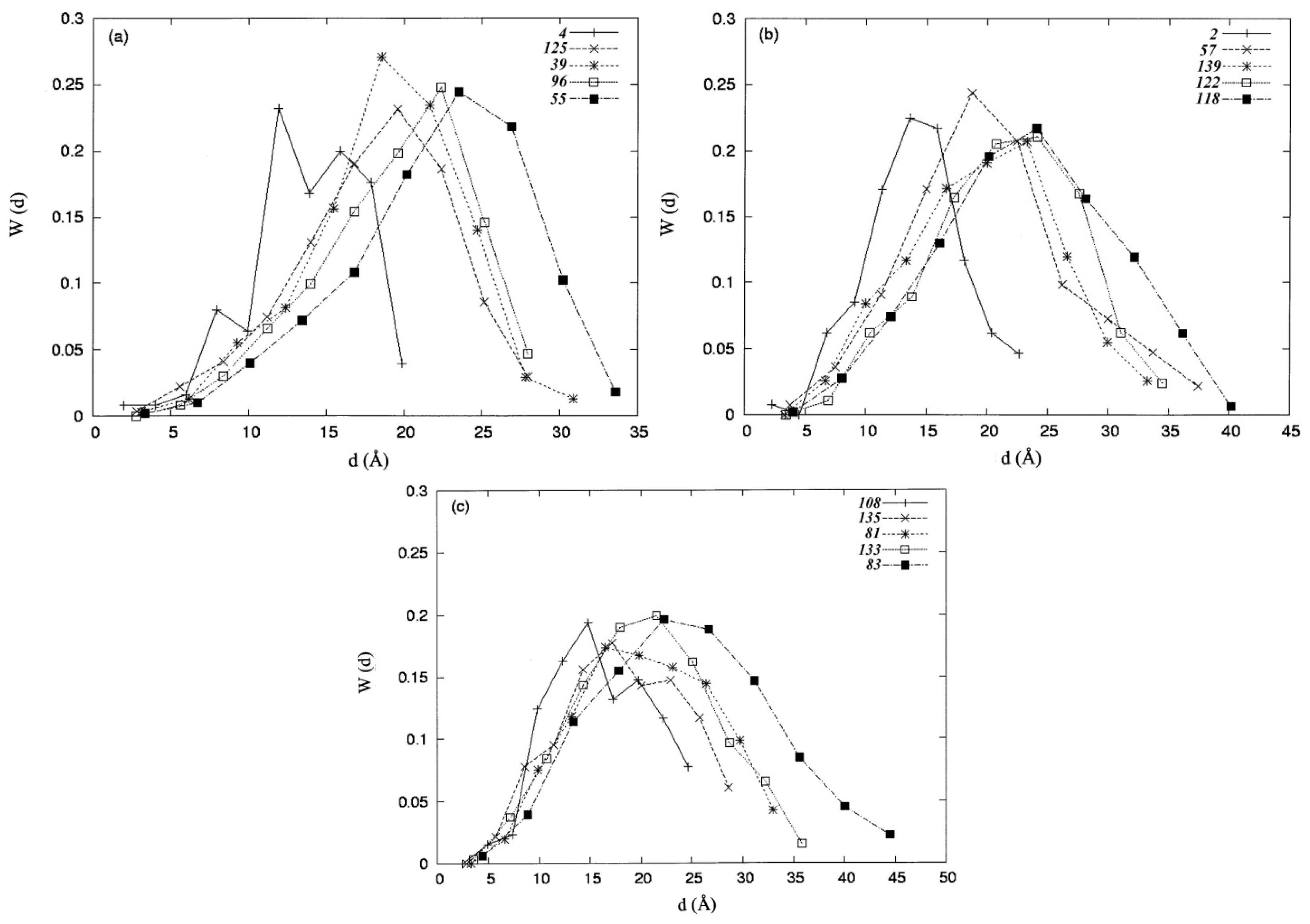
Figure 1. In order to select protein structures with diverse sizes and shapes, fifteen structures, as shown in
Table 1, were selected from these 150 proteins and divided into three groups, depending on the number of residues (
N) and the extent of asphericity (
δ).
The shape of a protein can be characterized in terms of eigenvalues of the radius of gyration tensor. The radius of gyration tensor
T is defined as follows [
28,
29]:
where
Ti = col (
xi, yi, zi) is the vector going from the origin at the protein center of mass vector to the position of the centroid of residue
i. The center of mass vector,
rCM, is defined by [
4]
where
Nr is the number of residues in the protein, and
ri is the position vector for the centroids of the amino-acid residues. The matrix
T can be diagonalized to obtain the three eigenvalues, α
i (
i = 1, 2, 3), of this tensor. The asphericity (
δ) [
28–
31] has been used to characterize protein shapes, and δ is computed as
If
δ = 0, the shape is a perfect sphere, the extent of asphericity can be referred as 0 <
δ < 1, and if
δ = 1, the shape is a rod. The shape parameter (
S) [
30,
31] has been used to quantify the whole shape of a protein, and
S is computed as
Where
If
S = 0, the shape is a perfect sphere, if
S < 0, the shape is oblate ellipsoid, and if
S > 0 the shape is prolate ellipsoid. The shape of proteins can also be represented by semiaxes [
32];
i.e.,
a = [5(
α1 +
α2)/2]
1/2 and
b = (5
α3)
1/2, where
αi was sorted according to increasing magnitude. If
a ≈
b, the shape is close to a sphere, and if
a <
b the shape is a prolate ellipsoid.
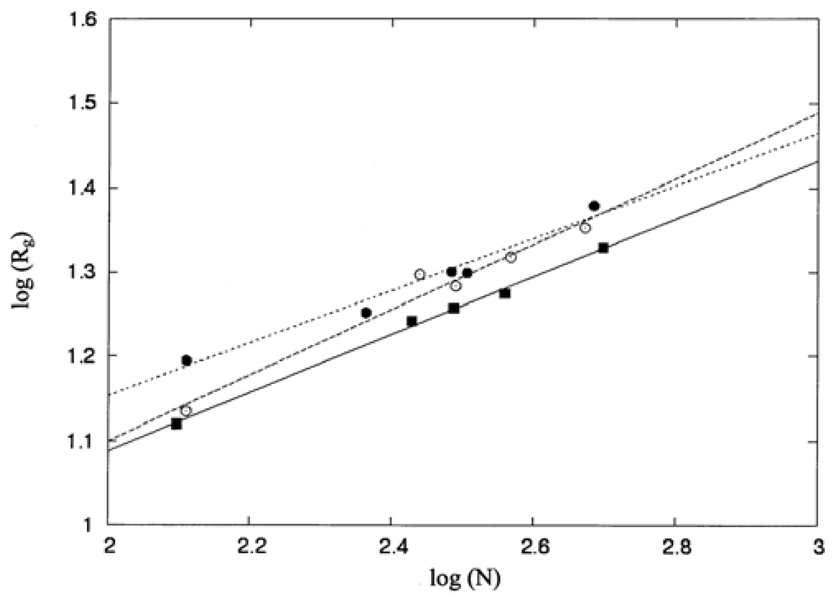
The molecular size of a protein can be probed using its mean square radius of gyration, 〈
Rg2〉, defined as follows [
33]:
The solvent accessible surface area (ASA) for each atom or for each residue in the proteins of interest was obtained using the computer program ASC [
34] with default parameters. The percentage of solvent accessibility,
p (%), was calculated as follows:
where
ASAX,folded is the ASA of X residue in the folded state of a given protein and
ASAX,G–X–G is the ASA of the corresponding residue X in tripeptide (Gly-X-Gly) with the extended state. The extended state (
ϕ =
Ψ = 180°) coordinates were generated using InsightII program [
35]. The Gly residues to either side of interest residue X can provide steric screening effects of neighboring residues in the simulated models, and such steric screening effects can reduce the values of ASAs calculated for the X residues in the extended state. The results of the ASA for each residue type X are shown in
Table 2Polar atoms were defined on the basis of the partial charges, which were assigned to atoms in a protein by the CHARMM program [
22]. In this work, three sets of partial charges, namely, |
qi| ≥ 0.25, 0.27, or 0.3 were assigned as polar atoms, and the remaining atoms were considered apolar. These three sets of partial charges were used to examine which one has the best correlation with the hydrophobicity consensus scale of Eisenberg [
5]. Polar and apolar ASAs of each residue were calculated by summing the ASA of the respective polar and apolar atoms in the residue. The hydrophobicity,
hi, for each amino-acid residue,
i, in a protein was calculated as follows:
where
ASAapo and
ASApo are the apolar and polar ASAs, respectively, in the residue. For a given protein, the
hi value of each residue, either selected from the hydrophobicity consensus scale of Eisenberg [
5], as shown in
Table 2, or calculated according to
Equation (8) was normalized by the following equation:
where
h̄ is the mean of the
hi for all residues in the protein, and σ(
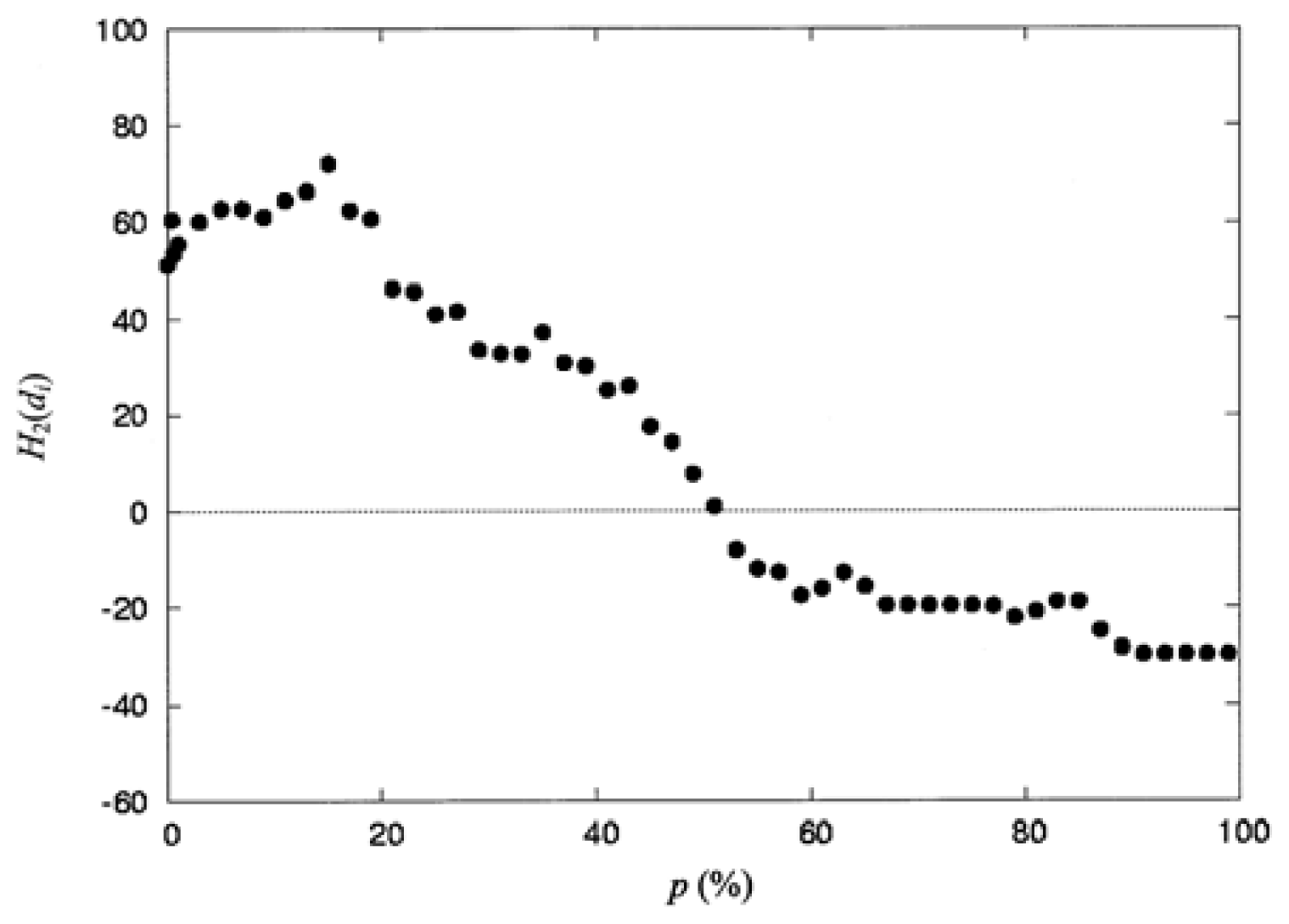
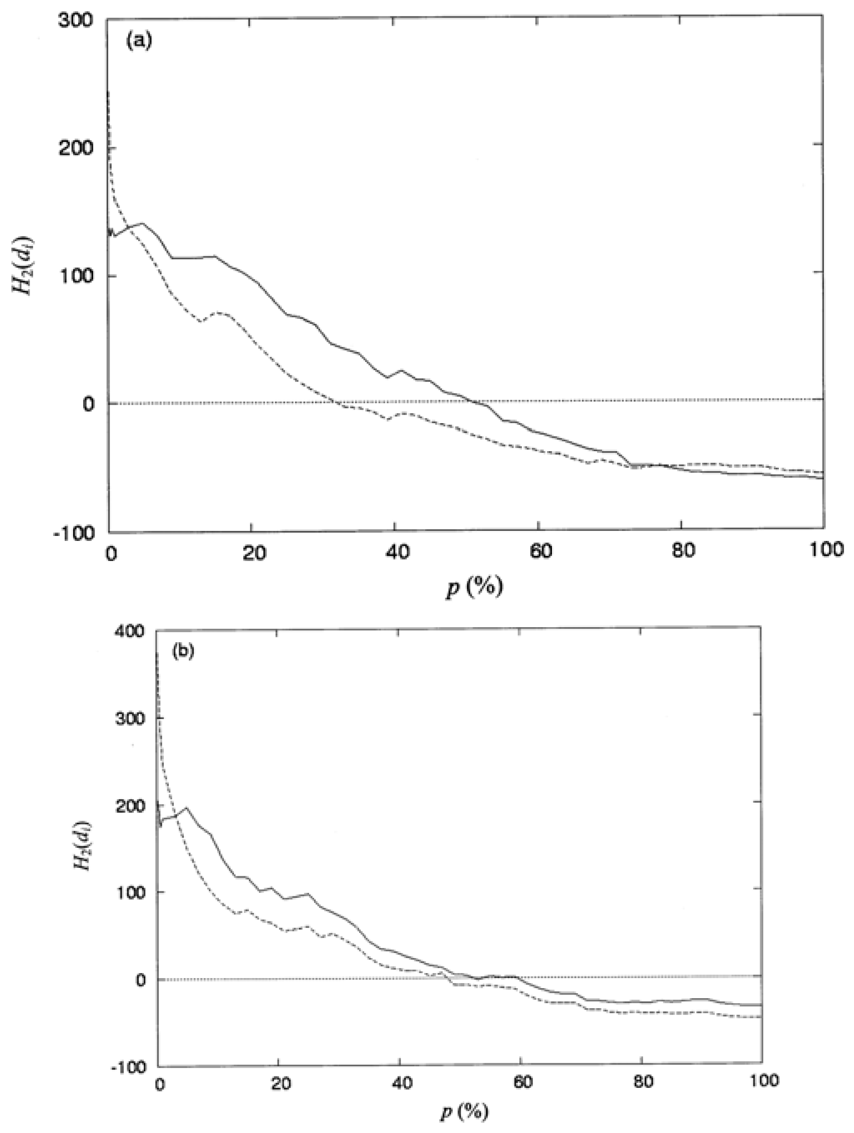
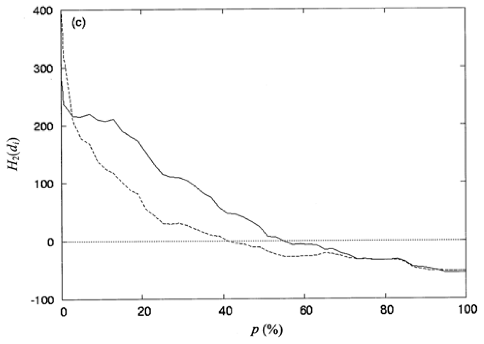
h) is their standard deviation. In this work, the second-order hydrophobic moment,
H2(d
i), per residue is similar to the works of Silverman [
4], given by
where np is the number of residues collected in the space defined by the percentage of solvent accessibility p (%), and di is the distance from the protein centroid to the centroid of residue i, in the space. Here, the protein centroid is the coordinates of its center of mass (CM). In this work, the space surface is dependent on p (%). When one selects a particular value of P (%), the number of residues np, is collected within the space. When a value of p (%) increases, the volume of the space is also increased and the number of residues np, residing in the space increases as well. The increment of p (%) is from 0 to 100%. Therefore, the spatial distribution of the second-order hydrophobic moment per residue, H2(di), is represented as a function of p (%).
The Pearson correlation coefficient [
36], R, was used to measure the correlation between the second-order moments as follows:
where
x denotes the second-order hydrophobic moment calculated with the
hi selected from the consensus scale (
Table 2), and
y denotes the second-order hydrophobic moment calculated with the
hi derived from the CHARMM partial atomic charges using
Equation (8). These
x and
y were normalized by
Equation (9).
x̄ and
ȳ denote the mean of
x and
y, respectively. In this work, this equation is also used to test whether the correlation coefficient between two data sets is statistically significant to determine the equation of the regression line. The correlation coefficient calculated with
Equation (11) is a linear correlation between the two data sets. If the correlation coefficient is close to 1, there is a very strong correlation between the two data sets.


