
QM/MM Calculations with deMon2k

Abstract
:1. Introduction—Why deMon2k?
- Variational fitting of the Coulomb potential
- Auxiliary density functional theory (ADFT)
- Adaptive numerical integration for exchange-correlation functionals
- Analytical molecular integral recurrence relations without limitation
- Half-numerical ECP and MCP integral recurrence relations
- MinMax self-consistent field (SCF) stabilization and acceleration
- Empirical dispersion corrections for all elements
- Geometry optimization with restricted step algorithm
- Hierarchical transition state finder
- Intrinsic reaction coordinate calculation
- Born-Oppenheimer molecular dynamics (BOMD) simulations
- Time-dependent ADFT (TD-ADFT)
- Auxiliary density perturbation theory (ADPT)
- Electric moments, polarizabilities and hyperpolarizabilities
- Nuclear magnetic resonance (NMR), infra-red (IR) and Raman spectra
- Thermodynamic data from polyatomic ideal gas model
- Population analyses (Mulliken, Löwdin, NBO, Bader)
- Topological analysis of molecular fields
- Interfaces for visualization software (Molden, Molekel, Vu)
- Portability to various computer platforms and operating systems
- Parallelized code (MPI)
- DFT optimized basis sets
- Automatic generation of adaptive auxiliary function sets
- Molecular mechanics energies, gradients and Hessian
- QM/MM interface to CHARMM, Cuby and PUPIL
- Constrained DFT and ADFT energies and gradients
- Asymptotic molecular integral expansions for mixed SCF
- Exact exchange with three-center electron repulsion integrals (ERIs)
- X-ray absorption and emission spectroscopy
- ROKS perturbation theory and Fukui functions
- Magnetizability, rotational g-tensor and spin-spin coupling constants
- BOMD property (NMR, , ) and analysis tools
- Non-iterative CPKS solver for perturbation theory
- VMT, LB94, B3LYP, PBE0 and M06-2X functionals
- Hirshfeld (iterative), Becke and Voronoi population analyses
- Plotting of Fukui functions, induced magnetic fields and perturbed or deformed densities
2. Recent Developments of deMon2k that Permit QM/MM Simulations of very Large Systems
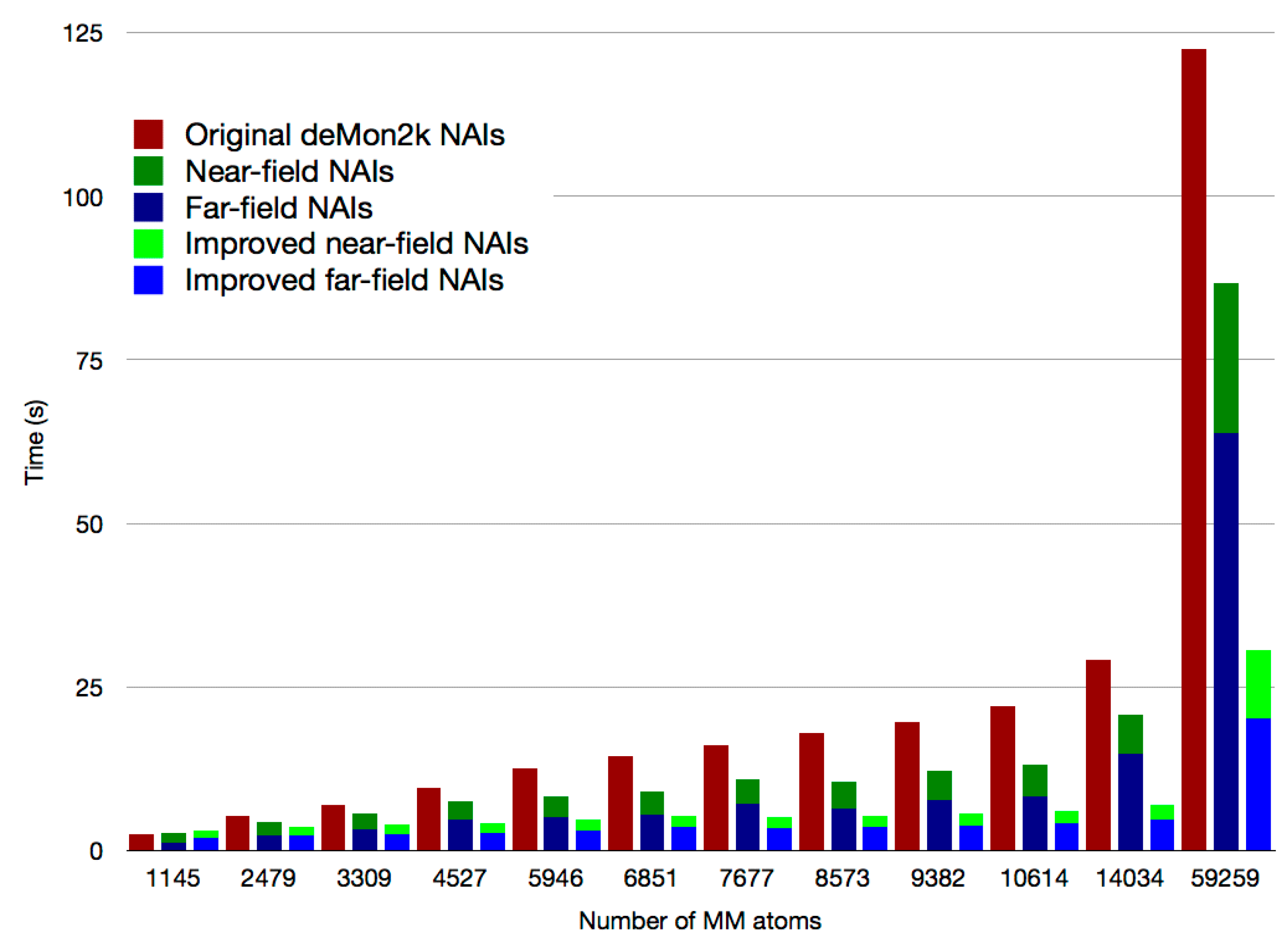
2.1. Asymptotic Expansion of QM/MM Embedding Integrals
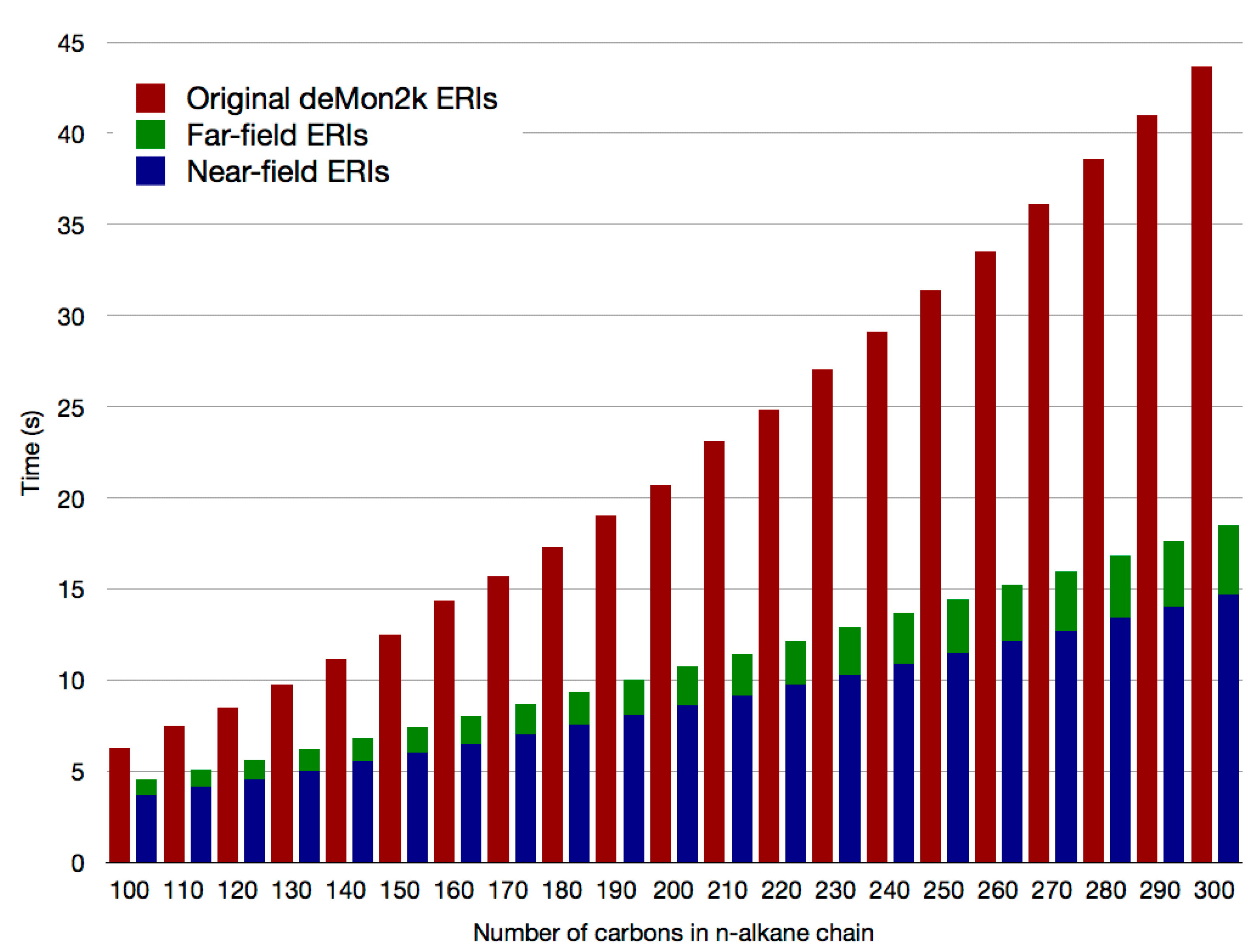
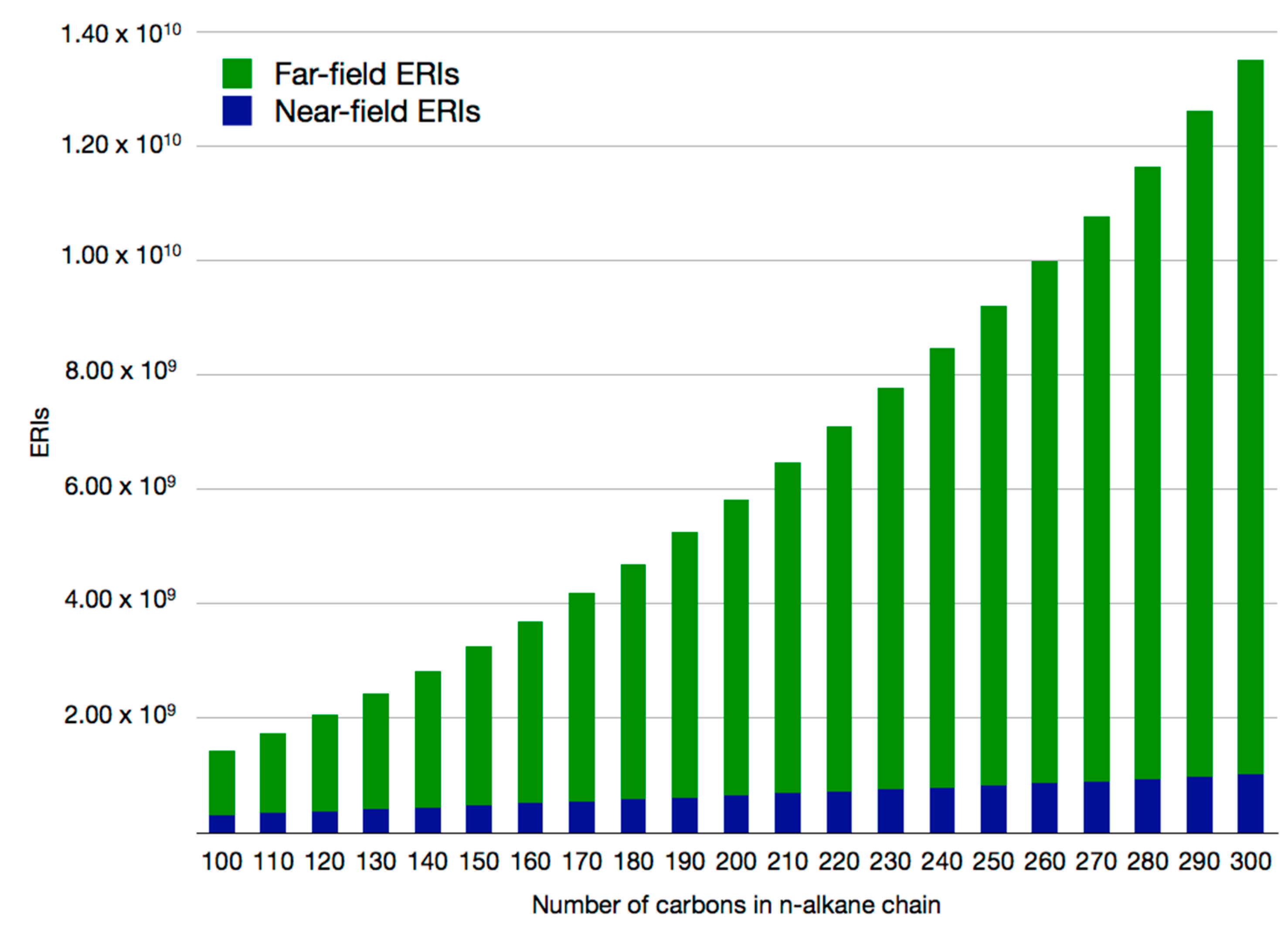
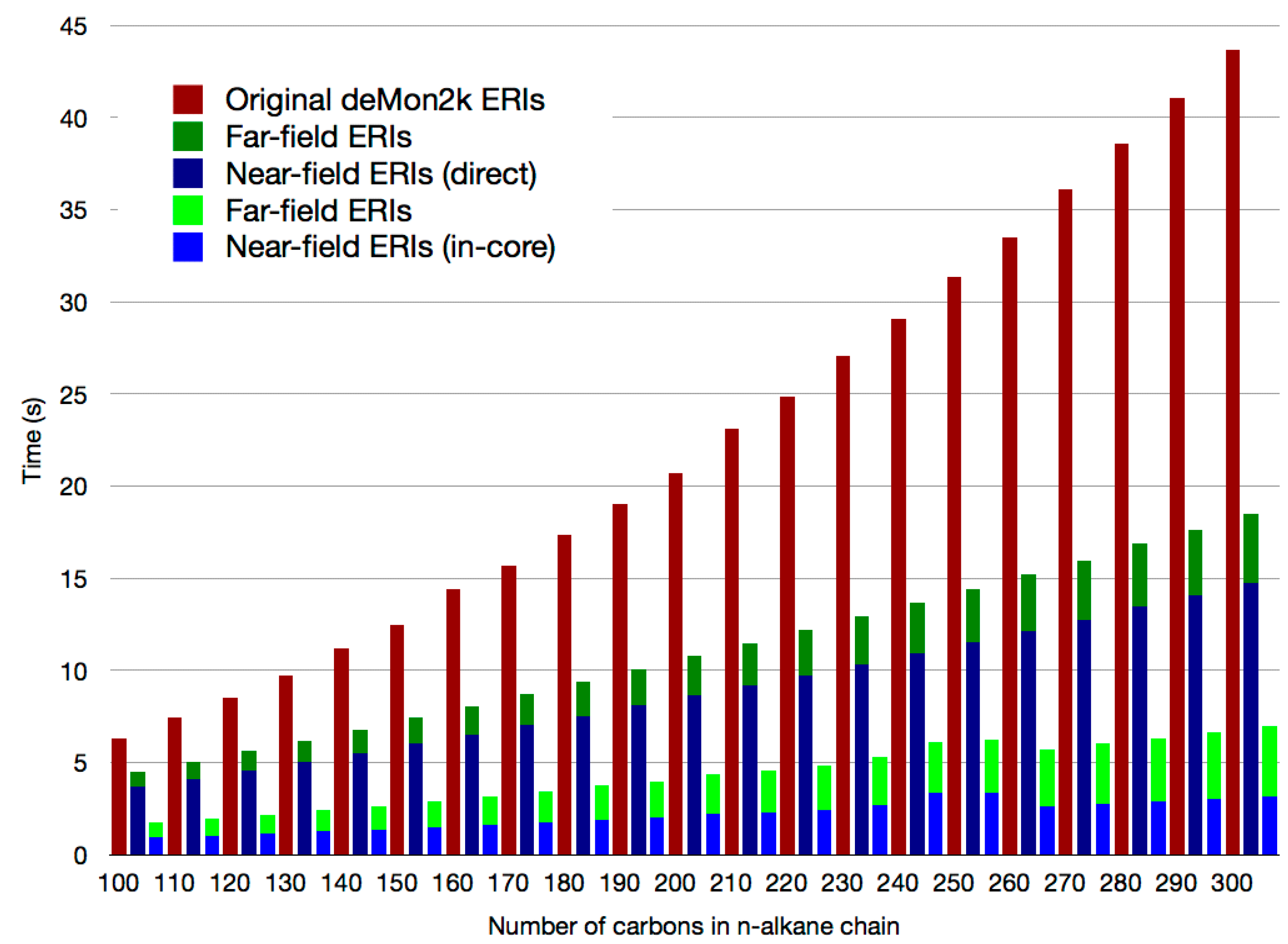
2.2. Double Asymptotic Expansion of Electron Repulsion Integrals

2.3. The Mixed SCF Scheme


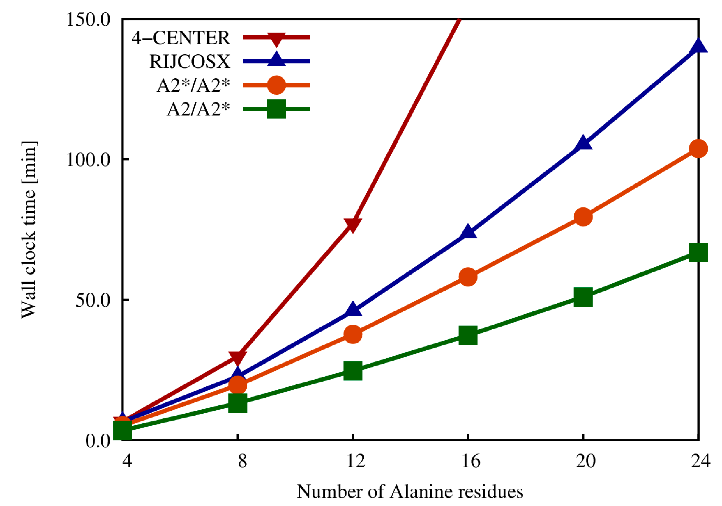
2.4. Exact Exchange in QM/MM Calculations
3. CHARMM-deMon Interface
3.1. Tested Force-Fields and General Details of MD Simulations with CHARMM-deMon2k
3.2. Free Energy Perturbation with CHARMM-deMon2k: Application to Ion Solvation

| System | Functional/Basis-Set | Sampling | ∆∆G |
|---|---|---|---|
| Cl-/Br- Perturbation | |||
| 16 QM + 234 MM | PBE98-PBE/def2-TZVPPD | 110 ps | 6.5 ± 0.2 |
| Available Experimental Data | |||
| Extra Thermodynamic Hypothesis | Schmid et al. [40] | 6.5 | |
| Aqueous Cluster Measurements | Tissandier et al. [41] | 6.4 | |
| Aqueous Cluster Measurements | Klots [42] | 3.3 | |
| Electrochemical Measurements | Gomer et al. [43] | 5.3 | |
| Na+/K+ Perturbation | |||
| 16 QM + 234 MM | PBE98-PBE/ DZVP-GGA | ~110 ps | −21.5 ± 0.2 |
| Available Experimental Data | |||
| Extra Thermodynamic Hypothesis | Schmid et al. [40] | −17.4 | |
| Aqueous Cluster Measurements | Tissandier et al. [41] | −17.2 | |
| Aqueous Cluster Measurements | Klotts [42] | −17.6 | |
| Electrochemical Measurements | Gomer et al. [43] | −17.6 | |
3.3. Hamiltonian Replica Exchange and the QM/MM Interface
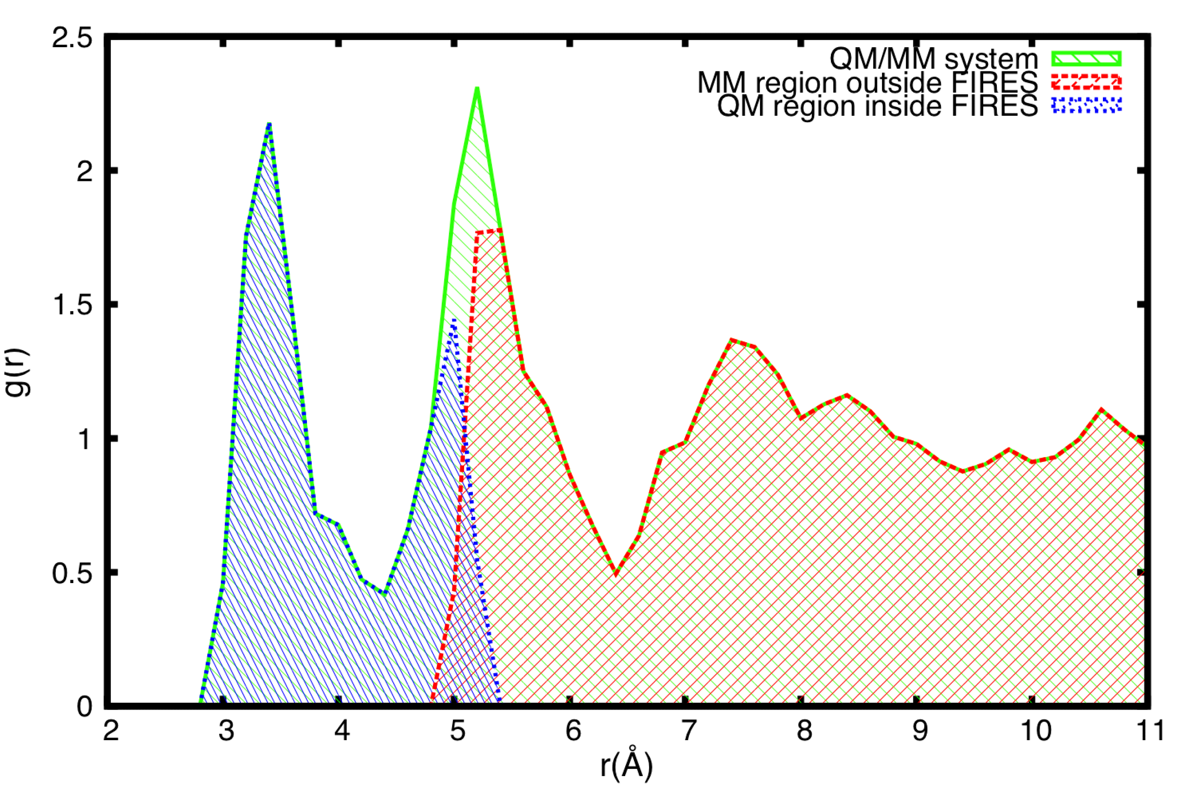
3.4. FIRES Separation: Flexible Boundaries between QM and MM Regions

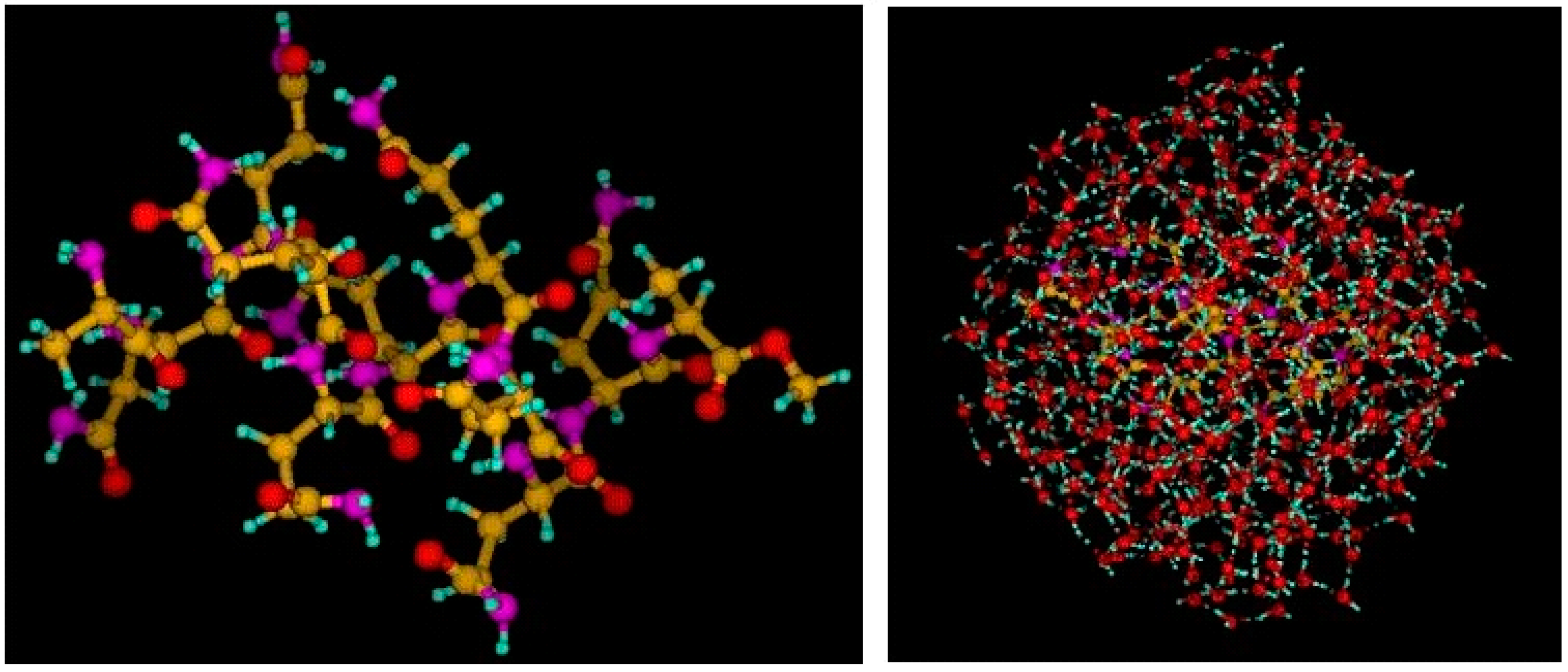
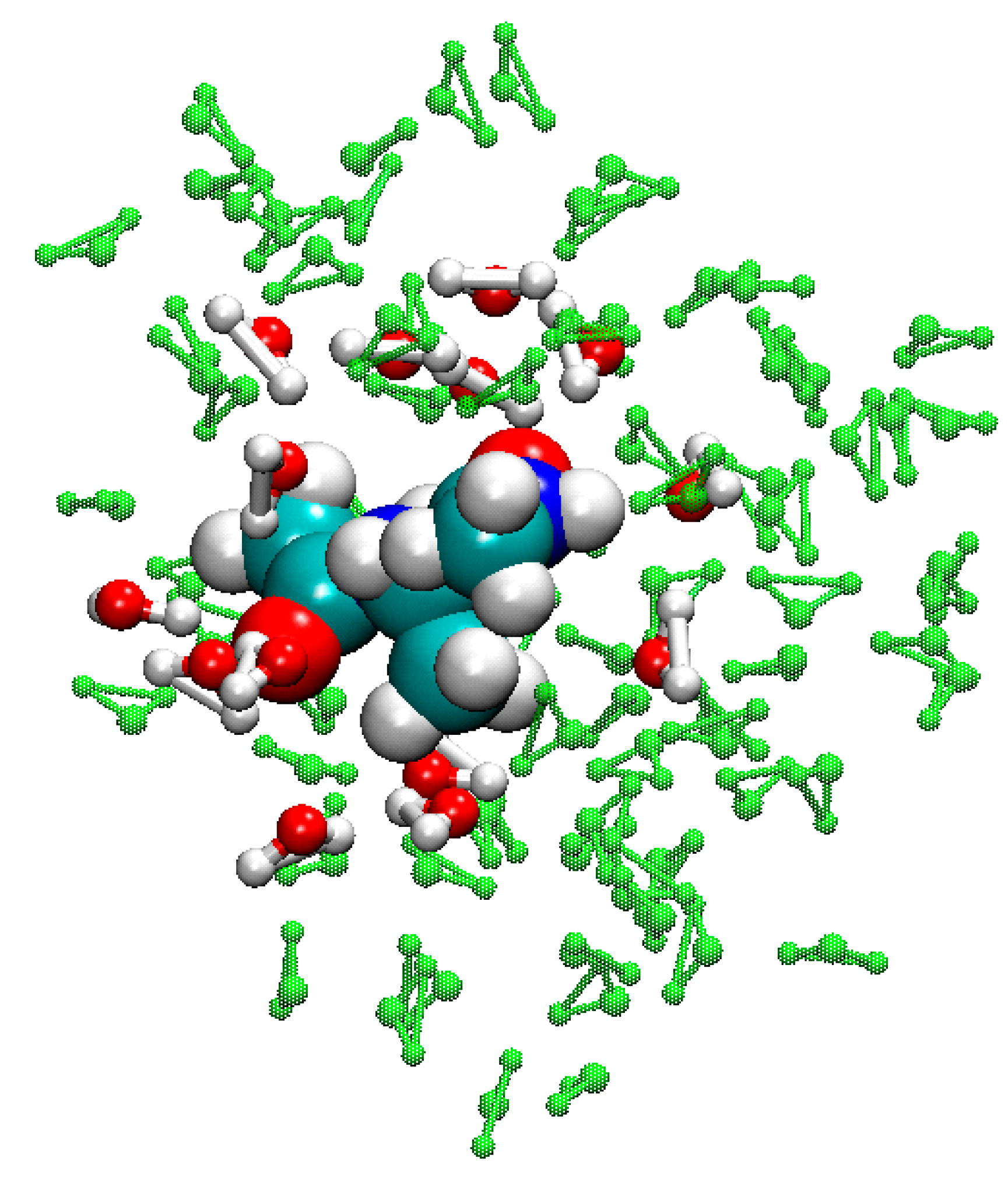
3.5. Example of FIRES for QM/MM Simulations of Biological Molecules in Water
4. In-deMon2k QM/MM
4.1. The in-deMon2k QM/MM Implementation
4.2. Benchmarking the in-deMon2k QM/MM Implementation
| Number of Processors | MM | QMd | QMm | QM/MMd | QM/MMm |
|---|---|---|---|---|---|
| 16 | 146 | 263,243 | 162,931 | 285,962 | 189,385 |
| 32 | 147 | 206,575 | 126,080 | 224,376 | 146,729 |
| 48 | 146 | 156,657 | 104,740 | 169,939 | 121,833 |
| 64 | 146 | 133,857 | 194,799 | 143,649 | 104,399 |
| 80 | 147 | 119,108 | 186,659 | 127,886 | 195,536 |
| 96 | 146 | 111,889 | 182,111 | 119,354 | 193,580 |

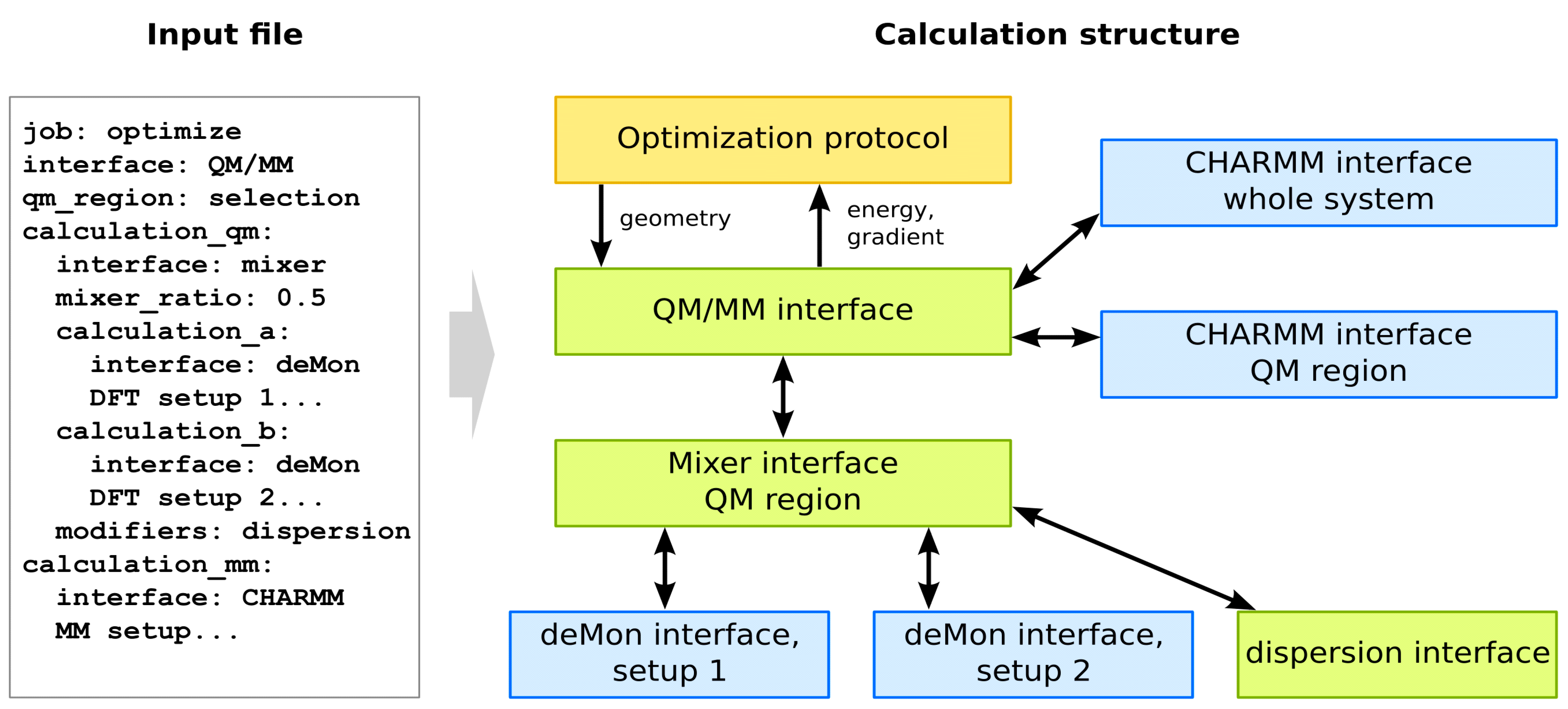
5. QM/MM with Cuby
5.1. Overview of Cuby

5.2. QM/MM Functionality in Cuby
5.3. deMon2k and CHARMM Interfaces
5.4. DFT-D in Cuby
5.5. Automated QM/MM Setup in Cuby
5.6. Other Cuby Functionality Used in QM/MM Calculations
5.7. Representative Applications
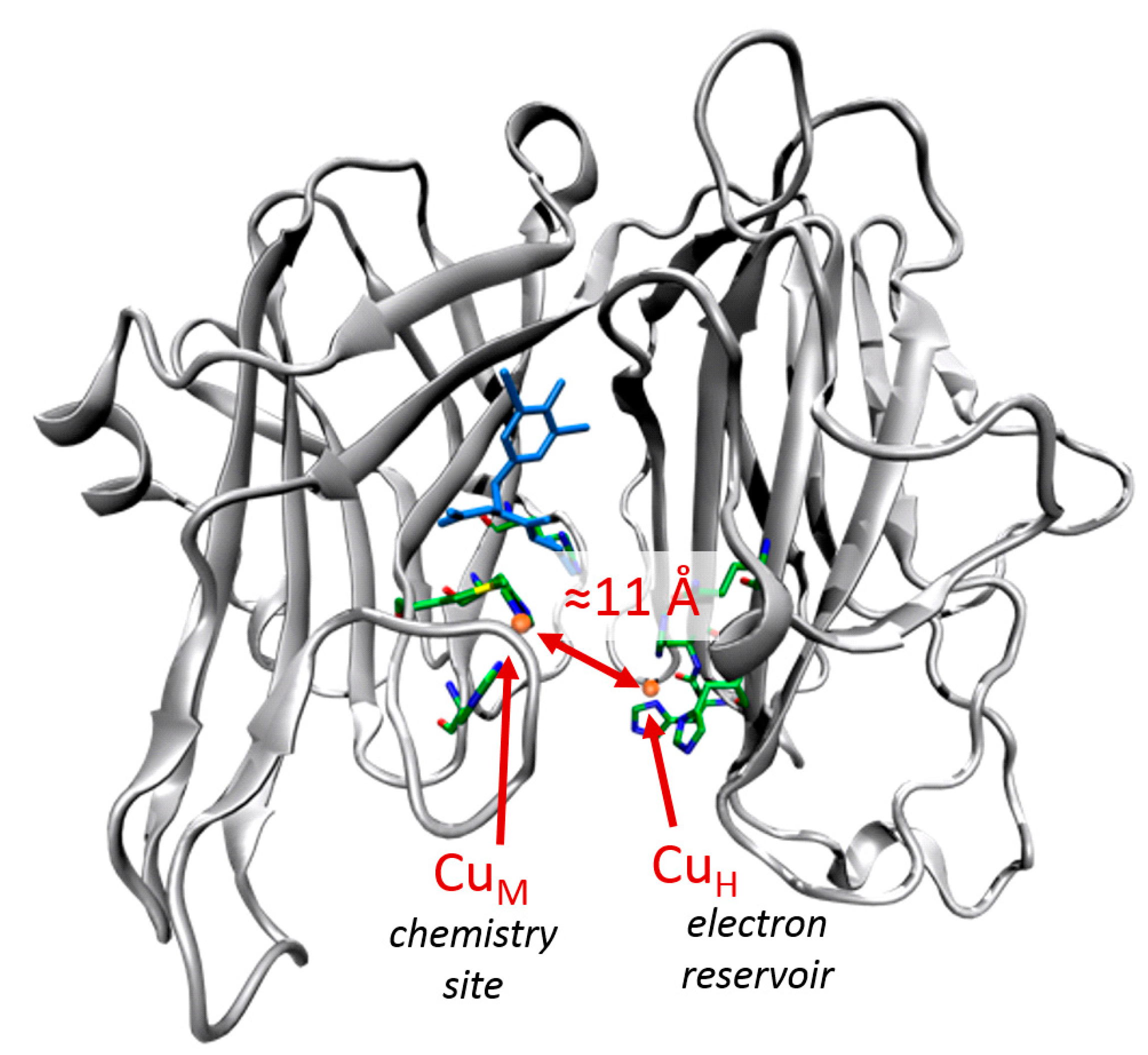
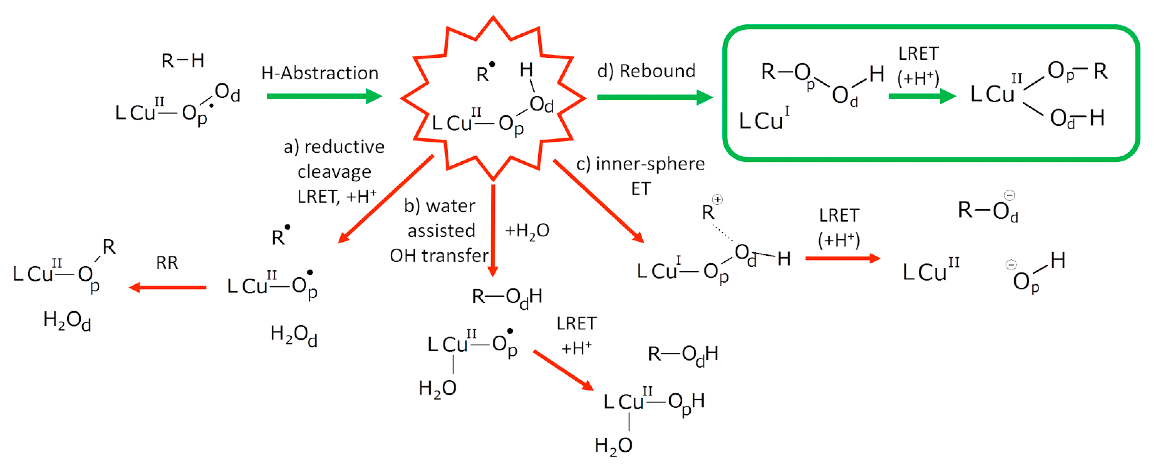
5.7.1. Investigation of Copper Monooxygenases

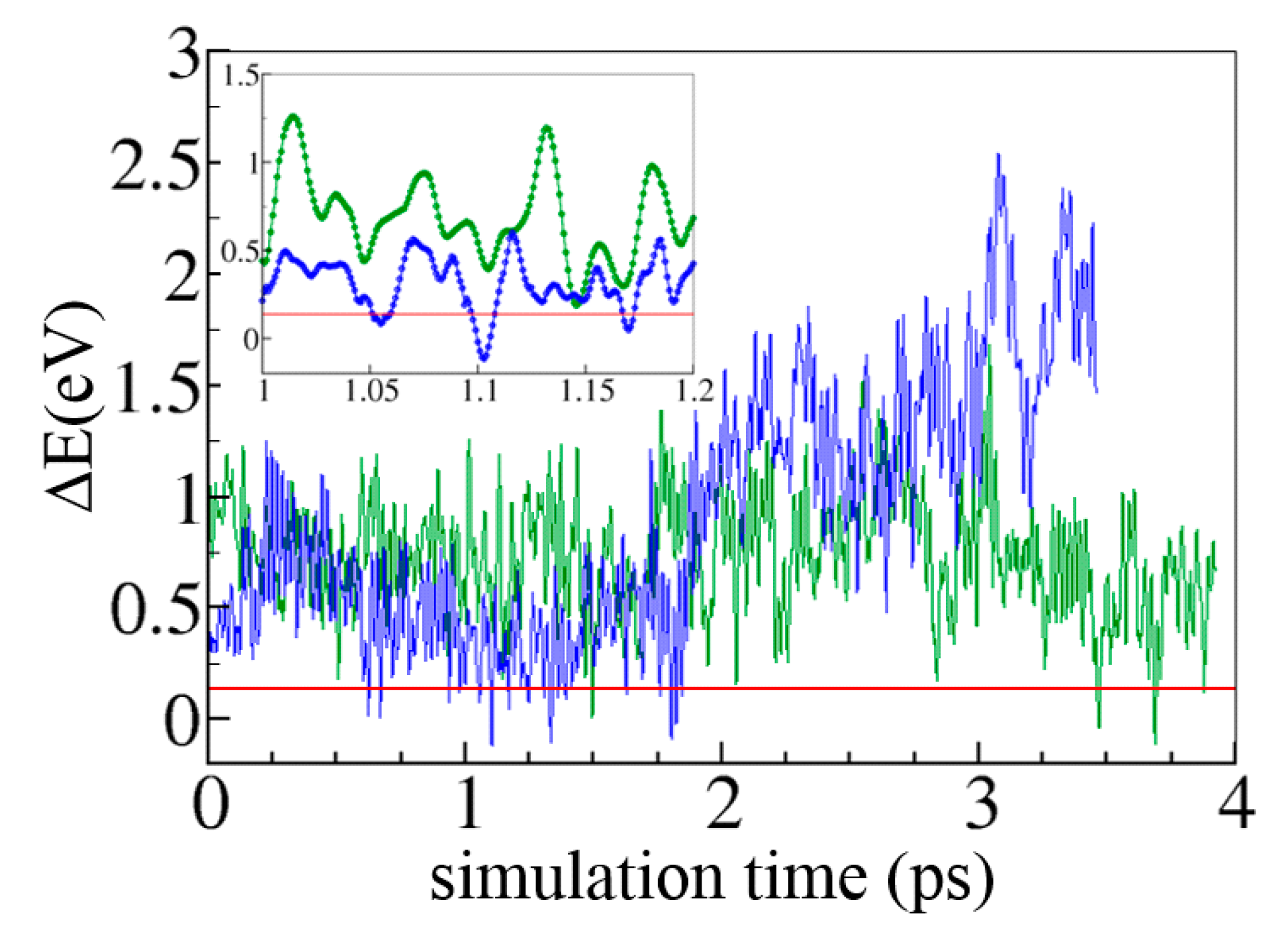
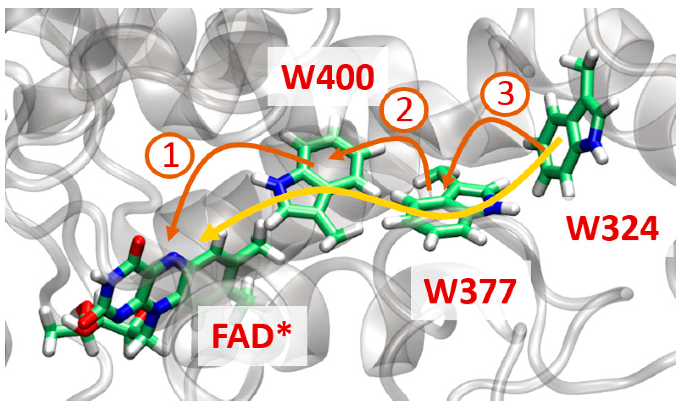
5.7.2. Ultrafast Electron Transfer in Cryptochromes

6. Concluding Remarks
Acknowledgments
Author Contributions
Conflicts of Interest
References
- Warshel, A.; Karplus, M. Calculation of Ground and Excited-State Potential Surfaces of Conjugated Molecules. 1. Formulation and Parametrization. J. Am. Chem. Soc. 1972, 94, 5612–5625. [Google Scholar]
- Warshel, A.; Levitt, M. Theoretical Studies of Enzymic Reactions—Dielectric, Electrostatic and Steric Stabilization of Carbonium-Ion in Reaction of Lysozyme. J. Mol. Biol. 1976, 103, 227–249. [Google Scholar] [CrossRef] [PubMed]
- Hu, H.; Yang, W.T. Free energies of chemical reactions in solution and in enzymes with ab initio quantum mechanics/molecular mechanics methods. Annu. Rev. Phys. Chem. 2008, 59, 573–601. [Google Scholar] [CrossRef] [PubMed]
- Senn, H.M.; Thiel, W. QM/MM methods for biological systems. Top. Curr. Chem. 2007, 268, 173–290. [Google Scholar]
- Senn, H.M.; Thiel, W. QM/MM Methods for Biomolecular Systems. Angew. Chem. Int. Ed. 2009, 48, 1198–1229. [Google Scholar] [CrossRef]
- Zhang, R.; Lev, B.; Cuervo, J.; Noskov, S.; Salahub, D. A Guide to QM/MM Methodology and Applications. Adv. Quantum Chem. 2010, 59, 353–400. [Google Scholar]
- Köster, A.; Geudtner, G.; Calaminici, P.; Casida, M.; Dominguez, V.; Flores-Moreno, R.; Gamboa, G.; Goursot, A.; Heine, T.; Ipatov, A.; et al. deMon2k, Version 3; Cinvestav: Mexico City, Mexico, 2011. Available online: http://www.demon-software.com.
- Geudtner, G.; Calaminici, P.; Carmona-Espindola, J.; del Campo, J.M.; Dominguez-Soria, V.D.; Moreno, R.F.; Gamboa, G.U.; Goursot, A.; Köster, A.M.; Reveles, J.U.; et al. deMon2k. Wiley Interdiscip. Rev. Comput. Mol. Sci. 2012, 2, 548–555. [Google Scholar] [CrossRef]
- Dunlap, B.; Connolly, J.; Sabin, J. Some approximations in applications of X-alpha theory. J. Chem. Phys. 1979, 71, 3396–3402. [Google Scholar] [CrossRef]
- Köster, A.; Reveles, J.; del Campo, J. Calculation of exchange-correlation potentials with auxiliary function densities. J. Chem. Phys. 2004, 121, 3417–3424. [Google Scholar] [CrossRef] [PubMed]
- Calaminici, P.; Janetzko, F.; Köster, A.; Mejia-Olivera, R.; Zuniga-Gutierrez, B. Density functional theory optimized basis sets for gradient corrected functionals: 3d transition metal systems. J. Chem. Phys. 2007, 126, 044108. [Google Scholar] [CrossRef] [PubMed]
- Köster, A. Hermite Gaussian auxiliary functions for the variational fitting of the Coulomb potential in density functional methods. J. Chem. Phys. 2003, 118, 9943–9951. [Google Scholar] [CrossRef]
- Köster, A.; Flores-Moreno, R.; Reveles, J. Efficient and reliable numerical integration of exchange-correlation energies and potentials. J. Chem. Phys. 2004, 121, 681–690. [Google Scholar] [CrossRef] [PubMed]
- Köster, A.; del Campo, J.; Janetzko, F.; Zuniga-Gutierrez, B. A MinMax self-consistent-field approach for auxiliary density functional theory. J. Chem. Phys. 2009, 130, 114106. [Google Scholar] [CrossRef] [PubMed]
- Geudtner, G.; Janetzko, F.; Köster, A.; Vela, A.; Calaminici, P. Parallelization of the deMon2k code. J. Comput. Chem. 2006, 27, 483–490. [Google Scholar] [CrossRef] [PubMed]
- Alvarez-Ibarra, A.; Köster, A.M. Double asymptotic expansion of three-center electronic repulsion integrals. J. Chem. Phys. 2013, 139, 024102. [Google Scholar] [CrossRef] [PubMed]
- Alvarez-Ibarra, A.; Köster, A.M.; Zhang, R.; Salahub, D.R. Asymptotic Expansion for Electrostatic Embedding Integrals in QM/MM Calculations. J. Chem. Theor Comput. 2012, 8, 4232–4238. [Google Scholar] [CrossRef]
- Alvarez-Ibarra, A.; Köster, A.M. A new mixed self-consistent field procedure. Mol. Phys. 2015. to be submitted. [Google Scholar]
- Calaminici, P.; Domingues-Soria, V.D.; Flores-Moreno, R.; Gamboa, G.U.; Geudtner, G.; Goursot, A.; Salahub, D.R.; Köster, A.M. Auxiliary Density Functional Theory: From Molecules to Nanostructures. In Handbook of Computational Chemistry; Leszczynski, J., Ed.; Springer-Verlag: Berlin/Heidelberg, Germany, 2011. [Google Scholar]
- Quintanar, C.; Caballero, R.; Köster, A. Long-range interactions in embedded ionic cluster calculations. Int. J. Quantum Chem. 2004, 96, 483–491. [Google Scholar]
- Alvarez-Ibarra, A. Modifications to the deMon2k Software to Implement Near- and Far-Fields. The Distance Calculation Has Been Moved from the Inner Shell Loops to the Atomic Loops, where the Near- and Far-Field Definitions Are now Calculated. This Reduces Dramatically the Repetitive Calculation of Powers and Square Roots Involved in the Distance Computation. CINVESTAV: Mexico City, Mexico, 2014. [Google Scholar]
- Mejía-Rodriguez, D.; Köster, A. Robust and Efficient Variational Fitting of Fock Exchange. J. Chem. Phys. 2014, 141, 124114. [Google Scholar] [CrossRef] [PubMed]
- Saebo, S.; Pulay, P. Local Treatment of Electron Correlation. Annu. Rev. Phys. Chem. 1993, 44, 213–236. [Google Scholar]
- Izsak, R.; Neese, F. An overlap fitted chain of spheres exchange method. J. Chem. Phys. 2011, 135, 144105. [Google Scholar] [CrossRef] [PubMed]
- Woodcock, H.L.; Hodošček, M.; Gilbert, A.T.B.; Gill, P.M.W.; Schaefer, H.F.; Brooks, B.R. Interfacing Q-Chem and CHARMM to perform QM/MM reaction path calculations. J. Comput. Chem. 2007, 28, 1485–1502. [Google Scholar] [CrossRef] [PubMed]
- Field, M.J.; Bash, P.A.; Karplus, M. A Combined Quantum-Mechanical and Molecular Mechanical Potential for Molecular-Dynamics Simulations. J. Comput. Chem. 1990, 11, 700–733. [Google Scholar] [CrossRef]
- Singh, U.C.; Kollman, P.A. A Combined Ab initio Quantum-Mechanical and Molecular Mechanical Method for Carrying out Simulations on Complex Molecular-Systems—Applications to the CH3Cl + Cl− Exchange-Reaction and Gas-Phase Protonation of Polyethers. J. Comput. Chem. 1986, 7, 718–730. [Google Scholar] [CrossRef]
- Maseras, F.; Morokuma, K. Imomm—A New Integrated Ab-Initio Plus Molecular Mechanics Geometry Optimization Scheme of Equilibrium Structures and Transition-States. J. Comput. Chem. 1995, 16, 1170–1179. [Google Scholar] [CrossRef]
- Murphy, R.B.; Philipp, D.M.; Friesner, R.A. A mixed quantum mechanics/molecular mechanics (QM/MM) method for large-scale modeling of chemistry in protein environments. J. Comput. Chem. 2000, 21, 1442–1457. [Google Scholar] [CrossRef]
- Pentikainen, U.; Shaw, K.E.; Senthilkumar, K.; Woods, C.J.; Mulholland, A.J. Lennard-Jones Parameters for B3LYP/CHARMM27 QM/MM Modeling of Nucleic Acid Bases. J. Chem. Theory Comput. 2009, 5, 396–410. [Google Scholar] [CrossRef]
- Riccardi, D.; Li, G.H.; Cui, Q. Importance of van der Waals interactions in QM/MM Simulations. J. Phys. Chem. B 2004, 108, 6467–6478. [Google Scholar] [CrossRef] [PubMed]
- Dapprich, S.; Komaromi, I.; Byun, K.S.; Morokuma, K.; Frisch, M.J. A new ONIOM implementation in Gaussian98. Part I. The calculation of energies, gradients, vibrational frequencies and electric field derivatives. J. Mol. Struct. (Theochem) 1999, 461, 1–21. [Google Scholar] [CrossRef]
- Lev, B.; Zhang, R.; de la Lande, A.; Salahub, D.; Noskov, S.Y. The QM-MM Interface for CHARMM-deMon. J. Comput. Chem. 2010, 31, 1015–1023. [Google Scholar] [PubMed]
- Lamoureux, G.; Roux, B. Absolute Hydration Free Energy Scale for Alkali and Halide Ions Established from Simulations with a Polarizable Force Field. J. Phys. Chem. B 2006, 110, 3308–3322. [Google Scholar] [CrossRef] [PubMed]
- Das, D.; Eurenius, K.P.; Billings, E.M.; Sherwood, P.; Chatfield, D.C.; Hodošček, M.; Brooks, B.R. Optimization of quantum mechanical molecular mechanical partitioning schemes: Gaussian delocalization of molecular mechanical charges and the double link atom method. J. Chem. Phys. 2002, 117, 10534–10547. [Google Scholar] [CrossRef]
- Lopes, P.E.M.; Huang, J.; Shim, J.; Luo, Y.; Li, H.; Roux, B.; MacKerell, A.D. Polarizable Force Field for Peptides and Proteins Based on the Classical Drude Oscillator. J. Chem. Theory Comput. 2013, 9, 5430–5449. [Google Scholar] [CrossRef] [PubMed]
- Li, G.H.; Zhang, X.D.; Cui, Q. Free energy perturbation calculations with combined QM/MM Potentials complications, simplifications, and applications to redox potential calculations. J. Phys. Chem. B 2003, 107, 8643–8653. [Google Scholar] [CrossRef]
- Lev, B.; Roux, B.; Noskov, S.Y. Relative Free Energies for Hydration of Monovalent Ions from QM and QM/MM Simulations. J. Chem. Theory Comput. 2013, 9, 4165–4175. [Google Scholar] [CrossRef]
- Rowley, C.N.; Roux, B. The Solvation Structure of Na+ and K+ in Liquid Water Determined from High Level ab Initio Molecular Dynamics Simulations. J. Chem. Theory Comput. 2012, 8, 3526–3535. [Google Scholar] [CrossRef]
- Schmid, R.; Miah, A.M.; Sapunov, V.N. A new table of the thermodynamic quantities of ionic hydration: Values and some applications (enthalpy-entropy compensation and Born radii). Phys. Chem. Chem. Phys. 2000, 2, 97–102. [Google Scholar] [CrossRef]
- Tissandier, M.D.; Cowen, K.A.; Feng, W.Y.; Gundlach, E.; Cohen, M.H.; Earhart, A.D.; Tuttle, T.R.; Coe, J.V. The proton’s absolute aqueous enthalpy and Gibbs free energy of solvation from cluster ion solvation data. J. Phys. Chem. A 1998, 102, 9308–9308. [Google Scholar] [CrossRef]
- Klots, C.E. Solubility of Protons in Water. J. Phys. Chem. 1981, 85, 3585–3588. [Google Scholar] [CrossRef]
- Gomer, R.; Tryson, G. Experimental-Determination of Absolute Half-Cell Emfs and Single Ion Free-Energies of Solvation. J. Chem. Phys. 1977, 66, 4413–4424. [Google Scholar] [CrossRef]
- Bankura, A.; Carnevale, V.; Klein, M.L. Hydration structure of salt solutions from ab initio molecular dynamics. J. Chem. Phys. 2013, 138, 014501. [Google Scholar] [CrossRef] [PubMed]
- Mahler, J.; Persson, I. A Study of the Hydration of the Alkali Metal Ions in Aqueous Solution. Inorg. Chem. 2012, 51, 425–438. [Google Scholar] [CrossRef] [PubMed]
- Faraldo-Gomez, J.D.; Roux, B. Characterization of conformational equilibria through Hamiltonian and temperature replica-exchange simulations: Assessing entropic and environmental effects. J. Comput. Chem. 2007, 28, 1634–1647. [Google Scholar] [CrossRef] [PubMed]
- Beglov, D.; Roux, B. Finite Representation of an Infinite Bulk System—Solvent Boundary Potential for Computer-Simulations. J. Chem. Phys. 1994, 100, 9050–9063. [Google Scholar] [CrossRef]
- Roux, B. Ion binding sites and their representations by reduced models. J. Phys. Chem. B 2012, 116, 6966–6979. [Google Scholar] [CrossRef] [PubMed]
- Li, H.; Ngo, V.A.; Da Silva, M.C.; Callahan, K.M.; Salahub, D.R.; Roux, B.; Noskov, S.Y. Representation of Ion-Protein Interactions using the Drude Polarizable Force-Field. J. Phys. Chem. B 2015. [Google Scholar] [CrossRef]
- Sherwood, A.; deVries, A.H.; Guest, M.F.; Shchreckenbach, G.; Catlow, C.R.A.; French, S.A.; Sokol, A.A.; Bromley, A.T.; Thiel, W.; Turner, A.J.; et al. QUASI: A general purpose implementation of the QM/MM approach and its application to problems in catalysis. J. Mol. Struct. (Theochem) 2003, 632, 1–28. [Google Scholar] [CrossRef]
- Cuby. Available online: http://cuby.molecular.cz (accessed on 25 February 2015).
- Torras, J.; Deumens, E.; Trickey, S.B. Perpsectives on simulations of chmo-mechanical phenomena. J. Comput. Aided Mater. Des. 2006, 13, 201–212. [Google Scholar] [CrossRef] [Green Version]
- Bertran, O.; Trickey, S.B.; Torras, J. Incorporation of deMon2k as a new parallel quantum mechanical code for the PUPIL system. J. Comput. Chem. 2010, 31, 2669–2676. [Google Scholar] [CrossRef] [PubMed]
- Hugosson, H.W.; Laio, A.; Maurer, P.; Röthlisberger, U. A comparative theoretical study of dipeptide solvation in water. J. Comput. Chem. 2006, 27, 672–684. [Google Scholar] [CrossRef] [PubMed]
- Kundrat, M.D.; Autschbach, J. Ab Initio and Density Functional Theory Modeling of the Chiroptical Response of Glycine and Alanine in Solution Using Explicit Solvation and Molecular Dynamics. J. Chem. Theory Comput. 2008, 4, 1902–1914. [Google Scholar] [CrossRef]
- Hu, H.; Lu, Z.Y.; Yang, W.T. QM/MM minimum free-energy path: Methodology and application to triosephosphate isomerase. J. Chem. Theory Comput. 2007, 3, 390–406. [Google Scholar] [CrossRef] [PubMed]
- Mineva, T.; Tsoneva, Y.; Kevorkyants, R.; Goursot, A. C-13 NMR chemical shift calculations of charged surfactants in water—A combined density functional theory (DFT) and molecular dynamics (MD) methodological study. Can. J. Chem. 2013, 91, 529–537. [Google Scholar] [CrossRef]
- Jorgensen, W.L.; Maxwell, D.S.; Tirado-Rives, J. Development and testing of the OPLS all-atom force field on conformational energetics and properties of organic liquids. J. Am. Chem. Soc. 1996, 118, 11225–11236. [Google Scholar] [CrossRef]
- Hu, H.; Lu, Z.Y.; Parks, J.M.; Burger, S.K.; Yang, W.T. Quantum mechanics/molecular mechanics minimum free-energy path for accurate reaction energetics in solution and enzymes: Sequential sampling and optimization on the potential of mean force surface. J. Chem. Phys. 2008, 128, 034105. [Google Scholar] [CrossRef] [PubMed] [Green Version]
- Flores-Moreno, R.; Alvarez-Mendez, R.; Vela, A.; Köster, A. Half-numerical evaluation of pseudopotential integrals. J. Comput. Chem. 2006, 27, 1009–1019. [Google Scholar] [CrossRef] [PubMed]
- DiLabio, G.A.; Wolkow, R.A.; Johnson, E.R. Efficient silicon surface and cluster modeling using quantum capping potentials. J. Chem. Phys. 2005, 122, 044708. [Google Scholar]
- Jardillier, N.; Goursot, A. One-electron quantum capping potential for hybrid QM/MM studies of silicate molecules and solids. Chem. Phys. Lett. 2008, 454, 65–69. [Google Scholar] [CrossRef]
- Kim, M.W.; Chelliah, Y.; Kim, S.W.; Otwinowski, Z.; Bezprozvanny, I. Secondary Structure of Huntingtin Amino-Terminal Region. Structure 2009, 17, 1205–1212. [Google Scholar] [CrossRef] [PubMed]
- Godbout, N.; Salahub, D.; Andzelm, J.; Wimmer, E. Optimization of Gaussian-type basis-sets for local spin-density calculations. 1. Boron through neon, optimization technique and validation. Can. J. Chem. 1992, 70, 560–571. [Google Scholar] [CrossRef]
- Dirac, P.A.M. Note on exchange phenomena in the Thomas atom. Proc. Camb. Philos. Soc. 1930, 26, 376–385. [Google Scholar] [CrossRef]
- Vosko, S.H.; Wilk, L.; Nusair, M. Accurate spin-dependent electron liquid correlation energies for local spin density calculations. Can. J. Phys. 1980, 58, 1200–1211. [Google Scholar] [CrossRef]
- Nosé, S. A unified formulation of the constant temperature molecular dynamics methods. J. Chem. Phys. 1984, 81, 511–519. [Google Scholar] [CrossRef]
- Hoover, W.G. Canonical dynamics: equilibrium phase-space distributions. Phys. Rev. A 1985, 31, 1695–1697. [Google Scholar] [CrossRef] [PubMed]
- Martyna, G.J.; Klein, M.L.; Tuckerman, M. Nosé-Hoover chains: The canonical ensemble via continuous dynamics. J. Chem. Phys. 1992, 97, 2635–2643. [Google Scholar] [CrossRef]
- Gamboa, G.; Vasquez-Perez, J.; Calaminici, P.; Köster, A. Influence of Thermostats on the Calculations of Heat Capacities From Born-Oppenheimer Molecular Dynamics Simulations. Int. J. Quantum Chem. 2010, 110, 2172–2178. [Google Scholar] [CrossRef]
- Jurecka, P.; Cerny, J.; Hobza, P.; Salahub, D.R. Density functional theory augmented with an empirical dispersion term. Interaction energies and geometries of 80 noncovalent complexes compared with ab initio quantum mechanics calculations. J. Comput. Chem. 2007, 28, 555–569. [Google Scholar] [PubMed]
- Grimme, S.; Antony, J.; Ehrlich, S.; Krieg, H. A consistent and accurate ab initio parametrization of density functional dispersion correction (DFT-D) for the 94 elements H-Pu. J. Chem. Phys. 2010, 132, 154104. [Google Scholar] [CrossRef] [PubMed]
- Duan, Y.; Wu, C.; Chowdhury, S.; Lee, M.C.; Xiong, G.M.; Zhang, W.; Yang, R.; Cieplak, P.; Luo, R.; Lee, T.; et al. A point-charge force field for molecular mechanics simulations of proteins based on condensed-phase quantum mechanical calculations. J. Comput. Chem. 2003, 24, 1999–2012. [Google Scholar] [CrossRef] [PubMed]
- Grimmelikhuijzen, C.J.P.; Williamson, M.; Hansen, G.N. Neuropeptides in cnidarians. Can. J. Zool. 2002, 80, 1690–1702. [Google Scholar] [CrossRef]
- Osborne, R.L.; Klinman, J.P. Insights into the Proposed Copper–Oxygen Intermediates that Regulate the Mechanism of Reactions Catalyzed by Dopamine β-Monooxygenase. In Copper Oxygen Chemistry; Karlin, K.D., Itoh, S., Eds.; Wiley: Hoboken, NJ, USA, 2011; pp. 1–22. [Google Scholar]
- Melia, C.; Ferrer, S.; Rezac, J.; Parisel, O.; Reinaud, O.; Moliner, V.; de la Lande, A. Investigation of the Hydroxylation Mechanism of Noncoupled Copper Oxygenases by Ab Initio Molecular Dynamics Simulations. Chem. Eur. J. 2013, 19, 17328–17337. [Google Scholar] [CrossRef] [PubMed]
- Evans, J.P.; Ahn, K.; Klinman, J.P. Evidence that dioxygen and substrate activation are tightly coupled in dopamine beta-monooxygenase—Implications for the reactive oxygen species. J. Biol. Chem. 2003, 278, 49691–49698. [Google Scholar] [CrossRef] [PubMed]
- Chen, P.; Solomon, E.I. Oxygen activation by the noncoupled binuclear copper site in peptidylglycine alpha-hydroxylating monooxygenase. Reaction mechanism and role of the noncoupled nature of the active site. J. Am. Chem. Soc. 2004, 126, 4991–5000. [Google Scholar] [CrossRef] [PubMed]
- De la Lande, A.; Parisel, O.; Gerard, H.; Moliner, V.; Reinaud, O. Theoretical exploration of the oxidative properties of a [(trenMe1)CuO2]+ adduct relevant to copper monooxygenase enzymes: Insights into competitive dehydrogenation versus hydroxylation reaction pathways. Chem. Eur. J. 2008, 14, 6465–6473. [Google Scholar] [CrossRef] [PubMed]
- Mouritsen, H.; Janssen-Bienhold, U.; Liedvogel, M.; Feenders, G.; Stalleicken, J.; Dirks, P.; Weiler, R. Cryptochromes and neuronal-activity markers colocalize in the retina of migratory birds during magnetic orientation. Proc. Natl. Acad. Sci. USA 2004, 101, 14294–14299. [Google Scholar] [CrossRef] [PubMed]
- Langenbacher, T.; Immeln, D.; Dick, B.; Kottke, T. Microsecond Light-induced Proton Transfer to Flavin in the Blue Light Sensor Plant Cryptochrome. J. Am. Chem. Soc. 2009, 131, 14274–14280. [Google Scholar] [CrossRef] [PubMed]
- Biskup, T.; Paulus, B.; Okafuji, A.; Hitomi, K.; Getzoff, E.D.; Weber, S.; Schleicher, E. Variable Electron Transfer Pathways in an Amphibian Cryptochrome: Tryptophan versus tyrosine-based radical pairs. J. Biol. Chem. 2013, 288, 9249–9260. [Google Scholar] [CrossRef] [PubMed]
- Řezáč, J.; Levy, B.; Demachy, I.; de la Lande, A. Robust and Efficient Constrained DFT Molecular Dynamics Approach for Biochemical Modeling. J. Chem. Theory Comput. 2012, 8, 418–427. [Google Scholar] [CrossRef]
- Cailliez, F.; Müller, P.; Gallois, M.; de la Lande, A. ATP binding and aspartate protonation enhance photoinduced electron transfer within plant cryptochromes. J. Am. Chem. Soc. 2014, 136, 12974–12986. [Google Scholar] [CrossRef] [PubMed]
- Kubas, A.; Hoffmann, F.; Heck, A.; Oberhofer, H.; Elstner, M.; Blumberger, J. Electronic couplings for molecular charge transfer: Benchmarking CDFT, FODFT, and FODFTB against high-level ab initio calculations. J. Chem. Phys. 2014, 140, 104105. [Google Scholar] [CrossRef] [PubMed]
- Oberhofer, H.; Blumberger, J. Revisiting electronic couplings and incoherent hopping models for electron transport in crystalline C-60 at ambient temperatures. Phys. Chem. Chem. Phys. 2012, 14, 13846–13852. [Google Scholar] [CrossRef] [PubMed]
- Tully, J.C. Mixed quantum-classical dynamics. Faraday Discuss. 1998, 110, 407–419. [Google Scholar] [CrossRef]
© 2015 by the authors. Licensee MDPI, Basel, Switzerland. This article is an open access article distributed under the terms and conditions of the Creative Commons Attribution license ( http://creativecommons.org/licenses/by/4.0/).
Share and Cite
Salahub, D.R.; Noskov, S.Y.; Lev, B.; Zhang, R.; Ngo, V.; Goursot, A.; Calaminici, P.; Köster, A.M.; Alvarez-Ibarra, A.; Mejía-Rodríguez, D.; et al. QM/MM Calculations with deMon2k. Molecules 2015, 20, 4780-4812. https://doi.org/10.3390/molecules20034780
Salahub DR, Noskov SY, Lev B, Zhang R, Ngo V, Goursot A, Calaminici P, Köster AM, Alvarez-Ibarra A, Mejía-Rodríguez D, et al. QM/MM Calculations with deMon2k. Molecules. 2015; 20(3):4780-4812. https://doi.org/10.3390/molecules20034780
Chicago/Turabian StyleSalahub, Dennis R., Sergei Yu. Noskov, Bogdan Lev, Rui Zhang, Van Ngo, Annick Goursot, Patrizia Calaminici, Andreas M. Köster, Aurelio Alvarez-Ibarra, Daniel Mejía-Rodríguez, and et al. 2015. "QM/MM Calculations with deMon2k" Molecules 20, no. 3: 4780-4812. https://doi.org/10.3390/molecules20034780