Abstract
This work studies the relationship between the energy allocated for transmitting a pair of correlated Gaussian sources over a two-user Gaussian broadcast channel with noiseless channel output feedback (GBCF) and the resulting distortion at the receivers. Our goal is to characterize the minimum transmission energy required for broadcasting a pair of source samples, such that each source can be reconstructed at its respective receiver to within a target distortion, when the source-channel bandwidth ratio is not restricted. This minimum transmission energy is defined as the energy-distortion tradeoff (EDT). We derive a lower bound and three upper bounds on the optimal EDT. For the upper bounds, we analyze the EDT of three transmission schemes: two schemes are based on separate source-channel coding and apply encoding over multiple samples of source pairs, and the third scheme is a joint source-channel coding scheme that applies uncoded linear transmission on a single source-sample pair and is obtained by extending the Ozarow–Leung (OL) scheme. Numerical simulations show that the EDT of the OL-based scheme is close to that of the better of the two separation-based schemes, which makes the OL scheme attractive for energy-efficient, low-latency and low-complexity source transmission over GBCFs.
1. Introduction
This work studies the energy-distortion tradeoff (EDT) for the transmission of a pair of correlated Gaussian sources over a two-user Gaussian broadcast channel (GBC) with noiseless, causal feedback, referred to as the GBCF. The EDT was originally proposed in [1] to characterize the minimum energy-per-source sample required to achieve a target distortion at the receiver, without constraining the source-channel bandwidth ratio. In many practical scenarios, e.g., satellite broadcasting [2], sensor networks measuring physical processes [3,4] and wireless body-area sensor networks [5,6,7], correlated observations need to be transmitted over noisy channels. Moreover, in various emerging applications, particularly in the context of the Internet of Things, the sampling rates are low; and hence, the channel bandwidth for transmission is much larger than the rate of the sources. Consequently, the main fundamental limitation for the communication system is the available energy per source sample. For example, in wireless body-area sensor networks, wireless computing devices located on, or inside, the human body measure physiological parameters, which typically exhibit correlations as they originate from the same source. These devices commonly have limited energy supply due to their size and are also subject to transmission power constraints due to safety restrictions, while bandwidth can be relatively large as communications takes place over short distances [8,9,10]. In this application, transmission of correlated parameters measured by a single sensor to different devices can be modeled as a BC with correlated sources. As an example for such a setting, consider a sensor measuring heart rate, as well as cardiac output (volume of blood outputted from the heart per unit time), which are correlated parameters (see, e.g., [10] (Section 2.6)), where the heart rate measurements are communicated to a smart watch (e.g., for the purpose of fitness tracking), while the cardiac output is communicated to a smart phone (e.g., for health monitoring and reporting purposes).
It is well known that for lossy transmission of a Gaussian source over a Gaussian memoryless point-to-point channel, either with or without feedback, when the source-channel bandwidth ratio is fixed and the average power is finite, then separate source and channel coding (SSCC) achieves the minimum possible average mean square error (MSE) distortion [11] (Theorem 3). In [1] (Cor. 1), it is further shown that SSCC is optimal also in the sense of EDT: for any target MSE distortion level, the minimal transmission energy is achieved by optimal lossy compression [12] (Chapter 13) followed by the most energy efficient channel code [13]. While [1] (Cor. 1) considered unbounded number of source samples, more recent works [14] (Theorem 9) and [15] showed that similar observations hold also for the point-to-point channel with a finite number of source samples. Except for a few special scenarios, e.g., [16,17,18] and the references therein, the optimality of SSCC does not generalize to multiuser networks, and a joint design of the source and channel codes can improve the performance.
An example for a setting in which SSCC is sub-optimal is the transmission of a pair of correlated Gaussian sources over a GBC where the bandwidths of the source and the channel match (i.e., on average, a single source sample pair is transmitted over a single use of the channel). The complete characterization of the achievable distortion pairs for this problem was given in [19], which also showed that a joint source-channel coding (JSCC) transmission scheme is optimal while separation-based schemes cannot achieve the optimal performance. JSCC for the transmission of correlated sources over GBCs with a source-channel bandwidth mismatch was recently studied in [20], where novel hybrid digital/analog coding schemes were proposed and shown to be superior to other schemes known in the literature. It should be noted that the transmission of correlated sources over GBCs is an important communications scenario, which applies to a vast number of practical applications, including broadcasting video [21,22], images [23] and physical measurements [24].
The impact of feedback on lossy JSCC over multiuser channels was considered in relatively few works. Several achievability schemes and a set of necessary conditions for losslessly transmitting a pair of discrete and memoryless correlated sources over a multiple-access channel (MAC) with feedback were presented in [25]. Lossy transmission of correlated Gaussian sources over a two-user Gaussian MAC with feedback was studied in [26], in which sufficient conditions, as well as necessary conditions for the achievability of an MSE distortion pair were derived for the case in which the source and channel bandwidths match. The work [26] also showed that for the symmetric setting, if the channel signal-to-noise ratio (SNR) is low enough, then uncoded transmission is optimal. While [26] considered source-channel coding with a unit bandwidth ratio, [1] studied the EDT for the transmission of correlated Gaussian sources over a two-user Gaussian MAC with and without feedback, when the bandwidth ratio is not restricted. Lastly, [27] improved the lower bound derived in [1] for the two-user Gaussian MAC without feedback and extended the results to more than two users.
While EDT analysis has gained some attention in recent years, the EDT of broadcast channels was considered only for GBCs without feedback. In particular, the work [15] studied the transmission of Gaussian sources over a GBC and characterized the energy-distortion exponents, namely, the exponential rate of decay of the square-error distortion as the available energy-to-noise ratio increases without bound. For GBCFs, the existing literature mainly focused on channel coding aspects, considering independent and uniformly distributed messages. A key work in this context is the work of Ozarow and Leung (OL) [28], which obtained inner and outer bounds on the capacity region of the two-user GBCF, by extending the point-to-point transmission strategy of Schalkwijk–Kailath (SK) [29]. The work [30] extended the OL scheme for two-user GBCFs by using estimators with memory (at the receivers) instead of the memoryless estimators used in the original OL scheme of [28]. In contrast to the point-to-point case [29], for GBCFs, both the scheme of [28] and the scheme of [30] are generally suboptimal. While the analysis and construction of the OL scheme [28] are carried out in an estimation theoretic framework, the works [31,32] approached the problem of channel coding for the GBCF within a control theoretic framework. Specifically, [32] proposed a transmission scheme based on linear quadratic Gaussian (LQG) control theory, that achieves rate pairs outside the achievable rate region of the OL code developed in [28]. Recently, it was shown in [33,34] that, for the two-user GBCF when the noise components at the receivers are mutually independent with equal variances, the LQG scheme of [32] achieves the maximal sum-rate among all possible linear-feedback schemes. Finally, it was shown in [35] that the capacity of GBCFs with independent noises at the receivers and only a common message cannot be achieved using a linear feedback scheme. Instead, the work [35] presented a capacity-achieving non-linear feedback scheme.
JSCC for the transmission of correlated Gaussian sources over GBCFs when the number of transmitted symbols is finite (referred to as the finite horizon regime) was previously considered in [36], which studied the minimal number of channel uses required to achieve a target MSE distortion pair. Three linear encoding schemes based on uncoded transmission were considered: the first scheme was a JSCC scheme based on the coding scheme of [28], to which we shall refer as the OL scheme; the second scheme was a JSCC scheme based on the scheme of [32], to which we shall refer as the LQG scheme; and the third scheme was a JSCC scheme whose parameters are obtained using dynamic programming (DP) (in the present work we discuss only the former OL and LQG schemes since the scheme based on DP becomes analytically and computationally infeasible as the number of channel uses goes to infinity). We note that linear and uncoded transmission, as implemented in the OL and in the LQG schemes, has important advantages, including low computational complexity, short coding delays and small storage requirements, which make this type of coding very desirable. We further note that although the LQG channel coding scheme of [32] for the two-user GBCF (with two messages) achieves the largest rate region out of all known channel coding schemes, in [36], it was shown that when the time horizon is finite, JSCC based on the OL scheme can achieve MSE distortion pairs lower than the JSCC based on the LQG scheme. In the present work, we analyze lossy source coding over GBCFs using SSCC and JSCC schemes based on a different performance metric: the EDT.
We note here that, as discussed above, noiseless feedback has been studied extensively in wireless Gaussian networks. An immediate benefit of this analysis is that the performance obtained for noiseless feedback serves as an upper bound on the performance for channels with noisy feedback. The analysis of noiseless feedback scenarios also leads to guidelines and motivation, which then can be applied to channels with noisy feedback. Indeed, the works [37,38], which studied channel coding for point-to-point Gaussian channels with noisy feedback and for GBCs with noisy feedback, respectively, considered transmission schemes, which are based on the SK [29] and on the OL schemes [28], respectively, originally developed for noiseless feedback scenarios. In [37,38], the noise in the feedback links was handled by applying modulo-lattice precoding in both the direct and feedback links. It is shown in [37,38] that, while having noise in the feedback links results in a performance degradation compared to the case of noiseless feedback [37] (Section V.D), many of the benefits of noiseless feedback can be carried over to the more practical setup of noisy feedback, thereby further motivating the current work. It follows that the analysis of noiseless feedback models provides practically relevant insights while facilitating simpler analysis.
Main contributions: In this work, the EDT for GBCFs is studied for the first time. We derive lower and upper bounds on the minimum energy per source pair required to achieve a target MSE distortion at each receiver, for the problem of transmitting a pair of Gaussian sources over a two-user GBCF, without constraining the number of channel uses per source sample. The new lower bound is based on cut-set arguments, while the upper bounds are obtained using three transmission schemes: two SSCC schemes and an uncoded JSCC scheme. The first SSCC scheme jointly compresses the two source sequences into a single bit stream, and transmits this stream to both receivers as a common message. The second SSCC scheme separately encodes each source sequence into two distinct bit streams, and broadcasts them via the LQG channel code of [32]. It is shown that in terms of the minimum energy-per-bit, the LQG code provides no gain compared to orthogonal transmission, from which we conclude that the first SSCC scheme, that jointly compresses the sequences into a single stream, is more energy efficient. As both SSCC schemes apply coding over multiple samples of the source pairs, they require high computational complexity, long delays and large storage space. We then consider the uncoded JSCC OL scheme presented in [36]. For this scheme, we first consider the case of fixed SNR and derive an upper bound on the number of channel uses required to achieve a target distortion pair. When the SNR approaches zero, the required number of channel uses grows, and the derived bound becomes tight. At the limiting scenario of , this provides a simple upper bound on the EDT. While our primary focus in this work is on the analysis of the three schemes mentioned above, such an analysis is a first step towards identifying schemes that would achieve improved EDT performance in GBCFs.
Numerical results indicate that the SSCC scheme based on joint compression achieves better EDT compared to the JSCC OL scheme; yet, the gap is quite small. Moreover, in delay-sensitive applications, there is a constraint on the maximal allowed latency in transmitting each source sample to the destination. In such scenarios, coding over large blocks of independent and identically distributed (i.i.d.) pairs of source samples is not possible, and instantaneous transmission of each observed pair of source samples via the JSCC-OL scheme may be preferable in order to satisfy the latency requirement, while maintaining high energy efficiency.
The rest of this paper is organized as follows: The problem formulation is detailed in Section 2. The lower bound on the minimum energy per source sample is derived in Section 3. Upper bounds on the minimum energy per source sample are derived in Section 4 and Section 5. Numerical results are detailed in Section 6, and concluding remarks are provided in Section 7.
2. Problem Definition
2.1. Notation
We use capital letters to denote random variables, e.g., X, and boldface letters to denote column random vectors, e.g., ; the element of a vector is denoted by , and we use , with , to denote . We use sans-serif fonts to denote matrices, e.g., . We use to denote differential entropy, to denote mutual information, and to denote a Markov chain, as defined in [12] (Chapters 9 and 2). We use , , , and to denote expectation, transpose, natural base logarithm, the set of real numbers and the set of non-negative integers, respectively. We let denote the set of functions such that . Finally, we define as the sign of , with .
2.2. Problem Setup
The two-user GBCF is depicted in Figure 1, with all of the signals being real. In this work, we consider the symmetric setting in which the sources have the same variances and the noises have the same variances. The encoder observes m i.i.d. realizations of a correlated and jointly Gaussian pair of sources , where , . The task of the encoder (transmitter) is to generate a transmitted signal that will facilitate decoding of the sequence of the source, , at the ith decoder (receiver), denoted by Rx, whose channel output at time k is given by:
for . The noise sequences , are i.i.d. over , with , where , .
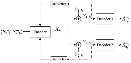
Figure 1.
Gaussian broadcast channel with correlated sources and feedback links. and are the reconstructions of and , respectively.
Let . The encoder maps the observed pair of source sequences and the noiseless causal channel outputs obtained through the feedback links into a channel input via: . Rx, , uses its channel output sequence to estimate via .
We study the symmetric GBCF with parameters , and define a code to be a collection of n encoding functions and two decoding functions , such that the MSE distortion satisfies:
and the energy of the transmitted signals satisfies:
Our objective is to characterize the minimal E, for a given target MSE D at each user, such that for all , there exist and a code. We call this minimal value the EDT and denote it by .
Remark 1 (Energy constraint vs. power constraint).
The constraint (3) reflects the energy per source sample rather than per channel use. Note that by defining , the constraint (3) can be equivalently stated as which is the well known average power constraint. Yet, since there is no constraint on the ratio between m and n, given a finite energy E, when the number of channel uses per source sample goes to infinity, the classical average power constraint goes to zero. We also note that can be obtained by evaluating the power-distortion tradeoff, namely, the minimal power required to achieve a given distortion at each receiver (see, e.g., [39] (Section II) for the definition of achievable distortion and power for a GBC with a given set of scenario parameters), in the limit . This approach was indeed used in [15] to derive energy-distortion exponents for GBCs without feedback. However, to the best of our knowledge, there are no tight bounds on the power-distortion tradeoff for GBCFs. Moreover, for the GBCF, we show next that directly characterizing leads to significantly simpler results.
3. Lower Bound on
Our first result is a lower bound on . First, we define as the rate-distortion function for the source variable , and as the rate distortion function for jointly compressing the pair of sources . Using [40] (Section III.B), we can write these functions explicitly as:
Note that [40] (Section III.B) uses the function as it allows for a different distortion constraint for each source. For the present setup, in which the same distortion constraint is applied to both sources, can be obtained by setting in [40] (Equation (8)), and thus, we use the simplified notation . Next, define:
The lower bound on the EDT is stated in the following theorem:
Theorem 1.
The EDT satisfies .
Remark 2 (Different approaches for deriving a lower bound).
The work [27] presented a novel technique for lower bounding the EDT in a Gaussian MAC. Applying this technique to the symmetric GBCF results in the lower bound reported in Theorem 1. The work [39] presented a lower bound on the distortion achievable in sending correlated Gaussian sources over a GBC (without feedback). This bound uses the entropy power inequality while relying on the fact that GBCs are degraded. As GBCFs are not degraded, it is not clear if the technique used in [39] can be used for deriving lower bounds on the EDT for GBCFs.
Proof of Theorem 1.
As we consider a symmetric setting, in the following, we focus on the distortion at Rx, and derive two different lower bounds. The first lower bound is obtained by identifying the minimal energy required in order to achieve an MSE distortion of D at Rx, while ignoring Rx. The second lower bound is obtained by considering the transmission of both sources over a point-to-point channel with two outputs and . We begin with the following lemma:
Lemma 1.
If for any , a code exists, then the rate-distortion functions in (4) are upper bounded by:
Proof.
The proof is provided in Appendix A. ☐
Now, for achievable fix and consider a code. For the right-hand side of (6a), we write:
where (a) follows by considering the point-to-point channel from to and noting that the capacity of this additive white Gaussian noise channel, subject to an input variance variance constraint , is . Thus, given with variance , then setting , it follows that ; (b) follows from changing the logarithm base and from the inequality ; and (c) follows by noting that (3) implies . Combining with (6a), we obtain , which implies that . Since this holds for every , we arrive at the first term on the right-hand-side (RHS) of (5).
Next, the RHS of (6b) can be upper bounded by considering a Gaussian single-input-multiple-output channel with two receive antennas. Then, the mutual information is upper bounded by the capacity of the channel subject to the variance of :
where (8) follows from [12] (Theorem 9.6.5), combined with [12] (Theorem 9.4.1) for jointly Gaussian random variables, and by defining and the covariance matrices and . To explicitly write , we note that for , and similarly, . We also have and . Thus, we obtain and . Plugging these expressions into (8) results in:
where the inequalities follow the same arguments as those leading to (7). Combining with (6b), we obtain , which implies that . Since this holds for every , we obtain the second term on the RHS of (5). This concludes the proof. ☐
In the next sections, we study three achievability schemes which lead to upper bounds on . While these schemes have simple constructions, analyzing their achievable EDT is novel and challenging.
4. Upper Bounds on E(D) via SSCC
SSCC in multiuser scenarios carries the advantages of modularity and ease of integration with the layered architecture, which is the fundamental design architecture in many practical communications systems. In this section, we analyze the EDT of two SSCC schemes. The first scheme takes advantage of the correlation between the sources and ignores the correlation between the noise components, while the second scheme ignores the correlation between the sources and aims at utilizing the correlation between the noise components.
4.1. The SSCC- Scheme
This scheme utilizes the correlation between the sources by first jointly encoding both source sequences into a single bit stream via the source coding scheme proposed in [41] (Theorem 6); see also [40] (Theorem III.1). For a given distortion D, the minimum required compression bit rate is given by the rate-distortion function stated in (4b). The bit stream generated through compression is then encoded via a channel code designed for sending a common message over the GBC (without feedback), and the corresponding codeword is transmitted to both receivers. Note that the optimal code for transmitting a common message over GBCFs with is not known, but, when , the optimal code for sending a common message over the GBCF is known to be the optimal point-to-point channel code which ignores the feedback [35] (Equation (13)). Thus, SSCC- uses the correlation between the sources, but ignores the correlation between the noises at the receivers. The following theorem characterizes the minimum energy per source sample achieved by this scheme.
Theorem 2.
The SSCC- scheme achieves the following EDT:
Proof.
The optimal rate for jointly encoding the source sequences into a single-bit stream is , given in (4b) [40] (Section III.B). Note that from this stream both source sequences can be recovered to within a distortion D. The encoded bit stream is then transmitted to both receivers via a capacity-achieving point-to-point channel code [12] (Theorem 10.1.1) (note that this code does not exploit the causal feedback [12] (Theorem 8.12.1)). Let denote the minimum energy-per-bit required for reliable transmission over the Gaussian point-to-point channel [13]. From [13] (p. 1025), we have . As the considered scheme is based on source-channel separation, the achievable EDT is given by , where is stated in (4b). This results in the EDT in (10). ☐
Remark 3 (EDT of GBC without feedback).
A basic question that may arise is about the EDT for transmitting a pair of correlated Gaussian sources over the GBC without feedback. The work [15] studied asymmetric GBCs, namely, when the noises have different variances, and used bounds derived in [39] to characterize the energy-distortion exponents. It is not clear whether the techniques used to derive the bounds in [39] can be used for the symmetric setting discussed in the current work. For the symmetric setting, the transmission of correlated Gaussian source over the GBC has been studied in [42]. Applying the results of [42] (Footnote 2) to the current case leads to the EDT of the SSCC- scheme, which indeed does not exploit feedback.
4.2. The SSCC- Scheme
This scheme aims at utilizing the correlation between the noises at the receivers, that is available at the encoder through the feedback links, for generating the channel symbols, while avoiding using the correlation between the sources for compression. As in this section we focus on separation-based schemes, the correlation between the noises at the receivers can be utilized only via the channel code. Our results show that in terms of EDT (or minimum required energy per pair of encoded bits), even the best known channel code cannot utilize the correlation between the noises at the receivers.
In the SSCC- scheme each of the source sequences is first compressed using the optimal rate-distortion source code for scalar Gaussian sources [12] (Theorem 13.3.2). Then, the resulting compressed bit streams are sent over the GBCF using the best known channel code for transmission over the GBCF, which is the LQG channel coding scheme of [32], that generally utilizes the correlation between the noises at the receivers, as is evident from [32] (IV.B) and in particular from [32] (Equations (23) and (24)). The following theorem characterizes the minimum energy per source sample required by this scheme.
Theorem 3.
The SSCC- scheme achieves the EDT:
Proof.
The encoder separately compresses each source sequence at rate , where is given in (4a). Thus, from each encoded stream the corresponding source sequence can be recovered to within a distortion D. Next, the two compressed bit streams are broadcast to their corresponding receivers using the LQG scheme of [32]. Let denote the minimum energy per pair of encoded bits required by the LQG scheme. is given in the following lemma:
Lemma 2.
For the symmetric setting, the minimum energy per pair of encoded bits required by the LQG scheme is given by:
Proof.
The proof is provided in Appendix B. ☐
Since two bit streams are transmitted, the achievable EDT is given by , yielding the EDT in (11). ☐
Remark 4 (SSCC-ρz vs. time-sharing)
Note that in (12) is independent of , and therefore, even though in general the LQG scheme is capable of utilizing the correlation between the noises at the receivers, in terms of minimum energy per pair of encoded bits it cannot (recall that the LQG scheme is the best known channel coding scheme for the GBCF). Therefore, is also independent of , and the SSCC- scheme does not take advantage of the correlation between the noises at the receivers to improve the minimum energy per source sample needed in the symmetric setting. Indeed, an EDT of can also be achieved by transmitting the two bit streams via time sharing over the GBCF without using the feedback. In this context, we recall that [43] (Prop. 1) also stated that in Gaussian broadcast channels without feedback, time sharing is asymptotically optimal as the power tends to zero.
Remark 5 (Relationship between , and ).
We observe that . For this relationship directly follows from the expressions of and . For the above relationship holds if the polynomial is positive. This is satisfied as the discriminant of is negative. We thus conclude that it is preferable to use the correlation between the sources than the correlation between the noise components. We further note that as , the gap between and is bounded. On the other hand, as , the gap between and is not bounded (note that when , the RHS of (5) is given by ).
Remark 6 (Relevance to more than two users).
The lower bound presented in Theorem 1 can be extended to the case of sources using the results of [41] (Theorem 1) and [44]. The upper bound of Theorem 2 can also be extended in a relatively simple manner to sources, again, using [41] (Theorem 1). The upper bound in Theorem 3 can be extended to sources by using the LQG scheme for [32] (Theorem 1), or by using time-sharing.
5. Upper Bound on E(D) via the OL Scheme
Next, we derive a third upper bound on by applying uncoded JSCC transmission based on the OL scheme [36] (Section 3). This scheme sequentially transmits the source pairs , , without source coding. Thus, the delay introduced by the OL scheme is significantly lower than the delay introduced by the schemes discussed in Section 4. We note that the OL scheme is designed for a fixed , and from condition (3) we obtain that . An upper bound on can now be obtained by first calculating the minimal number of channel uses required by the OL scheme to achieve the target distortion D, which we denote by , and then determining the required energy via .
5.1. JSCC Based on the OL Scheme
In the OL scheme, each receiver recursively estimates its intended source samples. At each time index, the transmitter uses the feedback to compute the estimation errors at the receivers at the previous time index, and transmits a linear combination of these errors. The scheme is terminated after channel uses, when the target MSE D is achieved at each receiver.
Setup and Initialization: Let be the estimate of at Rx after receiving the channel output , be the estimation error after k transmissions, and define . It follows that . Next, define to be the MSE at Rx after k transmissions, to be the correlation between the estimation errors after k transmissions, and . For initialization, set and ; thus, . Note that for this setup and initializations, we have .
Encoding: At the channel use the transmitter sends , and the corresponding channel outputs are given by (1).
Decoding: Each receiver computes , based only on via , which can be explicitly computed as in [28] (p. 669). Then, similarly to [45] (Equation (7)), the estimate of the source is given by . Let and . The instantaneous MSE is given by the recursive expression [28] (Equation (5)):
where the recursive expression for is given by [28] (Equation (7)):
Remark 7 (Initialization of the OL scheme).
Note that in the above OL scheme we do not apply the initialization procedure described in [28] (p. 669), as it optimizes the achievable rate rather than the distortion. Instead, we set and , thus, taking advantage of the correlation between the sources. Moreover, in Appendix C, it is explicitly shown that for the OL scheme, in the low SNR regime, the impact of the correlation between the sources on the distortion at the receivers lasts over a large number of channel transmissions. It thus follows that the proposed initialization clearly exploits the correlation between the sources.. We further note that [36] (Section III.B) considered several initialization methods for the OL scheme and showed that setting and outperforms the other studied initialization approaches.
Let denote the minimal energy per source pair required to achieve MSE D at each receiver using the OL scheme. Since in the OL scheme , we have . From (13) one observes that the MSE value at time instant k depends on and the MSE at time . Due to the non-linear recursive expression for in (14), it is very complicated to obtain an explicit analytical characterization for . For any fixed P, we can upper bound , and therefore , via upper bounding . In [36] (Theorem 1) we showed that , which leads to the upper bound: . However, when , the upper bound is not tight This can be seen by considering a numerical example: Let , and consider two possible values for P: and . Via numerical simulations one can find that , while the upper bound is 46,058. For we have , while the upper bound is 4,605,176. Thus, the gap between and the above bound increases as P decreases. For this reason, in the next subsection we derive a tighter upper bound on whose ratio to approaches 1 as . This bound is then used to derive a tighter upper bound on .
5.2. A New Upper Bound on
Following ideas from [1] (Theorem 7), we assume a fixed and approximate the recursive relationships for and given in (13) and (14) for small values of . We note that while [1] (Theorem 7) obtained only asymptotic expressions for and for , in the following we derive tight bounds for these quantities and obtain an upper bound on which is valid for small values of . Then, letting , the derived upper bound on yields an upper bound on , and therefore on .
First, define: and . We further define the positive quantities and :
and finally, we define the quantities:
For small values of , the following theorem provides a tight upper bound on :
Theorem 4.
Let P satisfy the conditions and . The OL scheme achieves MSE D at each receiver within channel uses, where, is given by:
Proof outline.
Let (otherwise replace with ). From [28] (p. 669) it follows that monotonically decreases with k until it crosses zero. Let be the largest time index k for which . In the proof of Theorem 4 we show that, for sufficiently small , . Hence, decreases until time and then it has a bounded magnitude (larger than zero). This implies that the behavior of is different in the regions and . Let be the MSE after channel uses. We first derive upper and lower bounds on , denoted by and , respectively. Consequently, we arrive at the two cases in Theorem 4: (17a) corresponds to the case of , while (17b) corresponds to the case . The detailed proof is provided in Appendix C. ☐
Remark 8 (Bandwidth used by the OL scheme).
Note that as , increases to infinity. Since, as , , it follows that as , . Assuming the source samples are generated at a fixed rate, this implies that the bandwidth used by the OL scheme increases to infinity as .
Remark 9 (Theorem 4 holds for non-asymptotic values of P).
Note that the conditions on P in Theorem 4 can be written as with depending explicitly on and . Plugging in (15) into the condition , we obtain the condition: . We note that, in this formulation the coefficients of , are all positive. Therefore, the left-hand-side (LHS) is monotonically increasing with P, and since is constant, the condition is satisfied if , for some threshold . Following similar arguments, the same conclusion holds for with some threshold instead of . Thus, by setting we obtain that the conditions in Theorem 4 restrict the range of power constraint values P for which the theorem holds for some .
5.3. An Upper Bound on
Next, we let , and use derived in Theorem 4 to obtain an upper bound on , and therefore on . This upper bound is stated in the following theorem.
Theorem 5.
Let . Then, , where
Proof.
We evaluate for . Note that , which implies that . To see why this holds, consider, for example, :
Since , and are constants, and since , we have . Now, since is constant we have . Taking the product of these two asymptotics we conclude that .
Now, for we bound the minimum as follows: First, for defined in (16g), we multiply both sides of (17a) by P. As , then, as , we obtain:
where (a) follows from (16f) by noting that , and therefore, when , . This implies that as we have . Finally, note that for we have .
Next, for we bound the minimum by first noting that since and , then . Now, for defined in (16h), multiplying both sides of (17b) by P, we obtain:
where (a) follows from the fact that , see (16a). This concludes the proof. ☐
Remark 10 (Performance for extreme correlation values).
Similarly to Remark 5, as , the gap between and is not bounded, which is in contrast to the situation for the OL-based JSCC for the Gaussian MAC with feedback, cf. [1] (Remark 6). When we obtain that , for all , which follows as the sources are independent. When and then , in this case we also have and .
Remark 11 (Comparison of the OL scheme and the separation-based schemes).
From (10) and (18), it follows that if then is given by:
Note that is independent of D in this range. Similarly, from (11) and (18) it follows that if then is independent of D and is given by:
Note that in both cases the gap decreases as decreases, which follows as the scenario approaches the transmission of independent sources. The gap also increases as decreases.
Remark 12 (Uncoded JSCC via the LQG scheme).
In this work, we do not include an analysis of the EDT of JSCC using the LQG scheme, , because JSCC-LQG does not lend itself to a concise analytical treatment, and, moreover, our numerical study demonstrated that, in terms of EDT, JSCC-LQG is generally inferior to JSCC-OL. To elaborate on these aspects, we first recall that the LQG scheme of [32] was already applied to the transmission of correlated Gaussian sources over GBCFs in [36] (Section IV). It follows from the derivations in [36] that is expressed as the solution of an optimization problem which does not have an explicit analytic solution. It is also shown in [36] that, for a finite duration of transmission and low transmission power, when the covariance matrix of the sources is different from the covariance matrix of the steady-state of the LQG scheme, then the JSCC-OL scheme outperforms the JSCC-LQG scheme, which stands in contrast to the results of [33] for the channel coding problem. This surprising conclusion carries over to the EDT as well. Indeed, using the results of [36] we carried out an extensive numerical study of JSCC-LQG, the outcome of which was that the JSCC-LQG scheme of [36] (Section IV) achieves roughly the same minimum energy as the SSCC- scheme. Since in Section 6 we show that the JSCC-OL scheme outperforms the SSCC- scheme in terms of the EDT, we decided to exclude the JSCC-LQG scheme from the numerical comparisons reported in Section 6.
6. Numerical Results
In the following, we numerically compare and . We set and consider several values of and . Figure 2a depicts and for , and for two values of : and . As is not a function of , it is plotted only once. It can be observed that when , then and are almost the same. This follows because when the correlation between the sources is low, the gain from utilizing this correlation is also low. Furthermore, when the gap between the lower bound and the upper bounds is evident. On the other hand, when , both SSCC- and OL significantly improve upon SSCC-. This follows as SSCC- does not take advantage of the correlation among the sources. It can further be observed that when the distortion is low, there is a small gap between OL and SSCC-, while when the distortion is high, OL and SSCC- require roughly the same amount of energy per source-pair sample. This is also supported by Figure 2c. We conclude that as the SSCC- scheme encodes over long sequences of source samples, it better exploits the correlation among the sources compared to the OL scheme.
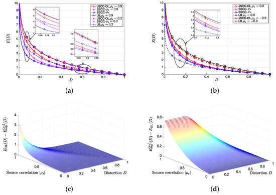
Figure 2.
Numerical results. (a) Upper and lower bounds on for , and . Solid lines correspond to , while dashed lines correspond to . (b) Upper and lower bounds on for . Solid lines correspond to , while dashed lines correspond to . (c) Normalized excess energy requirement of the OL scheme over the SSCC- scheme, . (d) Normalized excess energy requirement of the SSCC- scheme over the OL scheme, .
Figure 2b depicts and vs. D, for , and for . As and are not functions of , we plot them only once. It can be observed that when , and are very close to each other, as was analytically concluded in Remark 10. On the other hand, for the gap between the bounds is large.
Note that while analytically comparing , and for any D is difficult, our numerical simulations suggest the relationship , for all values of . For example, Figure 2c depicts the difference for , and for all values of D and . It can be observed that for low values of , or for high values of D, . On the other hand, when the correlation among the sources is high and the distortion is low, then the SSCC- scheme improves upon the OL scheme. When we can use (19) to analytically compute the gap between the energy requirements of the two schemes. For instance, at and the gap is approximately 3.173. Figure 2d depicts the difference for . It can be observed that larger results in a larger gap. Again we can use (20) to analytically compute the gap between the energy requirements of the two schemes for a certain range of distortion values: At and , the gap is approximately 0.744. Finally, as stated in Remark 12, the LQG scheme achieves approximately the same minimum energy as the SSCC- scheme, hence, OL is expected to outperform LQG. This is in accordance with [36] (Section VI), which shows that for low values of P, OL outperforms LQG, but, is in contrast to the channel coding problem in which the LQG scheme of [32] is known to achieve higher rates compared to the OL scheme of [28].
7. Conclusions and Future Work
In this work, we studied the EDT for sending correlated Gaussian sources over GBCFs, without constraining the source-channel bandwidth ratio. In particular, we first derived a lower bound on the minimum energy per source pair sample using information theoretic tools and then presented upper bounds on the minimum energy per source pair sample by analyzing three transmission schemes. The first scheme, SSCC-, jointly encodes the source sequences into a single bit stream, while the second scheme, SSCC-, separately encodes each of the sequences, thus, it does not exploit the correlation among the sources. We further showed that the LQG channel coding scheme of [32] achieves the same minimum energy-per-bit as orthogonal transmission, and therefore, in terms of the minimum energy-per-bit, it does not take advantage of the correlation between the noises at the receivers. We also concluded that SSCC- outperforms SSCC-.
The third scheme analyzed is the OL scheme for which we first derived an upper bound on the number of channel uses required to achieve a target distortion pair, which, in the limit , leads to an upper bound on the minimum energy per source pair sample. Numerical results indicate that SSCC- outperforms the OL scheme, as well. On the other hand, the gap between the energy requirements of the two schemes is rather small. We note that the SSCC- scheme implements coding over blocks of samples of source pairs, which introduces high computational complexity, large delays and requires a large amount of storage space. On the other hand, the OL scheme applies linear and uncoded transmission to each source pair sample separately, which requires low computational complexity, short delays and limited storage space. Our results demonstrate that the OL scheme provides an attractive alternative for energy efficient transmission over GBCFs.
Finally, we note that for the Gaussian MAC with feedback, OL-based JSCC is very close to the lower bound, cf. [1] (Figure 4), while, as indicated in Section 6, for the GBCF, the gap between the OL-JSCC and the lower bound is larger. This difference is also apparent in the channel coding problem for GBCFs, namely between the achievable rate region of the OL scheme and the tightest outer bound (note that while the OL strategy achieves the capacity of the Gaussian MAC with feedback [32] (Section V.A), for the GBCF the OL strategy is sub-optimal [28]). Therefore, it is interesting to see if the duality results between the Gaussian MAC with feedback and the GBCF, presented in [33,34] for the channel coding problem, can be extended to JSCC and if the approach of [33,34] facilitates a tractable EDT analysis. We consider this as a direction for future work.
Acknowledgments
This work was supported in part by the Israel Science Foundation under Grant 396/11 and by the European Research Council (ERC) through Starting Grant BEACON(Agreement #677854). Parts of this work were presented at the IEEE Information Theory Workshop (ITW), April 2015, Jerusalem, Israel [46], and at the IEEE International Symposium on Information Theory (ISIT), July 2016, Barcelona, Spain [47].
Author Contributions
Yonathan Murin developed this work in discussion with Yonatan Kaspi, Ron Dabora, and Deniz Gündüz. Yonathan Murin wrote the paper with comments from Yonatan Kaspi, Ron Dabora, and Deniz Gündüz. All authors have read and approved the final manuscript.
Conflicts of Interest
The authors declare no conflict of interest.
Abbreviations
The following abbreviations are used in this manuscript:
| EDT | Energy distortion tradeoff |
| GBC | Gaussian broadcast channel |
| GBC | Gaussian broadcast channel with feedback |
| JSCC | Joint source-channel coding |
| LHS | Left-hand side |
| LQG | Linear quadratic Gaussian |
| MAC | Multiple access channel |
| MSE | Mean square error |
| OL | Ozarow–Leung |
| RHS | Right-hand side |
| SK | Schalkwijk–Kailath |
| SNR | Signal-to-noise ratio |
| SSCC | Separate source-channel coding |
Appendix A. Proof of Lemma 1
We begin with the proof of (6a). From [12] (Theorem 13.2.1) we have:
Now, for any we write:
where (a) follows from the convexity of the mutual information in the conditional distribution , and from the assumption that the sources are memoryless; (b) is due to the non-negativity of mutual information combined with the chain rule for mutual information. Next, we upper bound as follows:
where (a) follows from the data processing inequality [12] (Section 2.8), by noting that ; (b) follows from the fact that conditioning reduces entropy, and from the fact that since the channel is memoryless, then depends on only through the channel input , see (1). By combining (A1)–(A3) we obtain (6a).
Next, we prove (6b). From [40] (Theorem III.1) we have:
Again, for any , we write:
where (a) is due to the convexity of the mutual information in the conditional distribution , and (b) follows from the memorylessness of the sources, the chain rule for mutual information, and from the fact that it is non-negative. Next, we upper bound as follows:
where (a) follows from the data processing inequality [12] (Section 2.8), by noting that we have ; (b) follows from the fact that conditioning reduces entropy, and from the fact that the channel is memoryless, thus, and depend on only through the channel input , see (1). By combining (A4)–(A6) we obtain (6b). This concludes the proof of the lemma.
Appendix B. Proof of Lemma 2: Minimum Energy-Per-Bit for the LQG Scheme
We first note that by following the approach taken in the achievability part of [48] (Theorem 1) it can be shown that for the symmetric GBCF with symmetric rates, the minimum energy-per-bit is given by:
where is the sum rate achievable by the LQG scheme. Let be the unique positive real root of the third order polynomial . From [32] (Equation (26)), for the symmetric GBCF, the achievable per-user rate of the LQG scheme is bits. We now follow the approach taken in [36] (Appendix A.3) and bound using Budan’s theorem [49].
Explicitly writing the derivatives of and evaluating the sequence , we have . Next, we let where is a real constant. Setting we obtain , , and . Note that we are interested in the regime which implies that . Now, for small enough we have . Furthermore, when we have . Clearly, for any , , and when , . Thus, letting , Budan’s theorem implies that when , the number of roots of in the interval is 1. From Descartes’ rule [50] (Section 1.6.3), we know that there is a unique positive root, thus, as this holds for any , we conclude that . Plugging the value of into (A7), and considering the sum-rate, we obtain:
This concludes the proof.
Appendix C. Proof of Theorem 4
First, note that if , we can replace with , which changes only the sign of in the joint distribution of the sources. Note that changing the sign of in (14) only changes the sign of while remains unchanged. Hence, in (13) is not affected by changing the sign of . Therefore, in the following we assume that . To simplify the notation we also omit the dependence of on P and D, and write . For characterizing the termination time of the OL scheme we first characterize the temporal evolution of . From [28] (p. 669), decreases (with k) until it crosses zero. Let , regardless of whether the target MSE was achieved or not. We begin our analysis with the case .
Appendix C.1. The Case of KOL ≤ Kth
From (14) we write the (first order) Maclaurin series expansion [50] (Chapter 7.3.3.3) of in the parameter P:
where is the remainder of the first order Maclaurin series expansion. The following lemma upper bounds :
Lemma A1.
For any k, we have , where is defined in (15).
Proof.
Let . From Taylor’s Theorem [50] (Subsection 6.1.4.5) it follows that , for some . In the following we upper bound , for : Let , , , , and (note that in order to simplify the expressions we ignore the dependence of , and on k). Using (14), the expression can now be explicitly written as , from which we obtain:
Since , we lower bound the denominator of in the range by . Next, we upper bound each of the terms in the numerator of . For the coefficient of we write , where the inequality follows from the fact that . For the coefficient of we write . For the coefficient of x we write . Finally, for the constant term we write . Collecting the above bounds on the terms of the numerator, and the bound on the denominator, we obtain , concluding the proof of the lemma. ☐
Note that for we have . Hence, (A9) together with Lemma A1 imply that, for we have:
Next, note that the function satisfies:
The lower bound on follows from the fact that is concave, and the upper bound is obtained via: . When then we have , hence . Thus, we can combine the lower and upper bounds on , and the bound on to obtain the following lower and upper bounds on :
Now, recalling that , the fact that the bound in (A11) does not depend on k results in the following upper bound on :
Next, using the fact that for , we rewrite (A9) as follows:
which implies that for we have:
Observe that , which follows from the fact that is lower and upper bounded independent of P and (see (A10)), and from the fact that . Next, we focus on the LHS of (A13) and write:
Since , it follows that is continuous, differentiable and bounded over , which implies that there exists a constant such that:
The constant is upper bounded in the following Lemma A2. Note that (A15) constitutes an upper bound on the maximal magnitude of the difference between and .
Lemma A2.
The constant , in (A15), satisfies: .
Proof.
Since , the mean-value theorem [50] (Section 6.1.4) implies: . Writing explicitly we have: . To maximize over , we compute . Setting requires . Since for all the roots of are complex (the determinant of is equal to .), then is not equal to 0 in the interval , and hence its maximal value is achieved at one of the boundaries of the interval [0,1]. This concludes the proof of the lemma. ☐
Next, we write the LHS of (A14) as follows:
where (a) follows from (A14); (b) follows from (A15) which implies that , and from Lemma A2; (c) follows from explicitly calculating the integral, and by multiplying (A12) by the RHS of (A11) to bound the summation, and then using the upper bounds (A11) and (A12) which leads to an upper bound on the second summation by , which is defined in (16b). By following arguments similar to those leading to (A16) the summation at the LHS of (A14) can be lower bounded via:
Next, consider again the RHS of (A13). Using the bound (A10) and Lemma A1, we can write:
where (a) follows from (A12), the LHS of (A10) and Lemma A2, and from the definitions of and in Section 5.2. Plugging the lower bound (A17) and the upper bound (A18) into (A13) we arrive at an upper bound on when :
We emphasize that the above expressions hold only for , and we note that these expressions depend on . As is unknown, in the following we bound its value. For this purpose, we set in (13) and write:
where (a) follows from the first order Maclaurin series expansion of in the parameter P, and is the remainder term. Note that this holds for any , irrespective whether it is smaller or larger than . The following lemma upper bounds :
Lemma A3.
For any k we have , where is defined in (15).
Proof outline.
We follow the technique used in the proof of Lemma A1. We let , and use Taylor’s theorem to write for some . Then, we upper bound in the range . ☐
Next, we focus on the first summation on the RHS of (A20): From (A9), and for , we have . Hence, we write the first summation on the RHS of (A20), for as:
Similarly to (A16) we write:
where
Here, in step (a) is obtained as , where is upper bounded as in (A12), and follows from bounding , where is found using a similar approach to the one in the proof of Lemma A2. Then, applying arguments similar to those leading to (A16), we plug the upper bound on stated in the RHS of (A11), and combine with the bound on to obtain . Step (b) follows from the fact that which implies that is increasing with , and therefore, its maximal value is achieved at .
For the second term on the RHS of (A21), noting that for , we write:
Now, we consider the second term on the RHS of (A20). From (A12) and Lemma A3 we obtain:
Therefore, from (A20)–(A24) using the definition of in (16d), we obtain:
By following similar arguments for lower bounding , we also obtain:
From (A25a), we can extract the following lower bound on : . Similarly, from (A25b), we can extract the following upper bound on : . Up to this point we assumed that and therefore . Hence, we restricted our attention only to values of D for which , which is satisfied for . We conclude that if , we can obtain an upper bound on plugging into (A19):
This corresponds to the bounds (17a). In the next subsection, we consider the case of .
Appendix C.2. The Case of KOL > Kth
For upper bounding when , we first derive an upper bound on for . From (A9) we have for any k:
where (a) follows from Lemma A1, and (b) follows since is non-negative. Thus, we can use the upper bound in (A10) to further bound:
Note that this bound holds for every k, regardless of the value of . Further note that the condition implies that . The following lemma uses (A27) to bound .
Lemma A4.
For it holds that .
Proof.
We first recall that while . Therefore, the bound combined with implies that as well as . From [28] (p. 669) we have that if then , and if then . Note that these statements hold for every k. We now prove by induction the statement: Suppose , for , then . Note that the induction assumption is satisfied for . If , then , which implies that since . If , then , which again, implies that since . Thus, by induction we conclude that . ☐
Next, we characterize a lower bound on the distortion achieved after time steps. Recall that for we have , where is defined in Appendix C.1. By setting , we obtain . Thus, constitutes a lower bound on .
Now, we are ready to analyze the case of . We first note that (A20) holds for any value of . Hence, we write:
For the second term on the RHS of (A28), we write:
where (a) follows from Lemma A3, as the lemma holds for any k, and from the fact that . Since the sum in (A20) is negative, we require , which results in . Now, we write (A28) as:
and note that since (A20)–(A25) hold for , then replacing with in (A20)–(A25) and with we can bound:
where we used the fact that . Thus, to obtain an upper bound on we write:
Finally, plugging instead of in (A19), we obtain an upper bound on . Since the function in (A19) monotonically decreases with x, using the lower bound , we obtain an explicit upper bound on . Combining this upper bound on with (A30) we obtain the following upper bound on :
where since , dividing by changes the direction of the inequality. This concludes the proof.
References
- Jain, A.; Gündüz, D.; Kulkarni, S.R.; Poor, H.V.; Verdú, S. Energy-distortion tradeoffs in Gaussian joint source-channel coding problems. IEEE Trans. Inf. Theory 2012, 58, 3153–3168. [Google Scholar] [CrossRef]
- Alagöz, F.; Gür, G. Energy efficiency and satellite networking: A holistic overview. Proc. IEEE 2011, 99, 1954–1979. [Google Scholar] [CrossRef]
- Rault, T.; Bouabdallah, A.; Challal, Y. Energy efficiency in wireless sensor networks: A top-down survey. Comput. Netw. 2014, 67, 104–122. [Google Scholar] [CrossRef]
- He, T.; Krishnamurthy, S.; Stankovic, J.A.; Abdelzaher, T.; Luo, L.; Stoleru, R.; Yan, T.; Gu, L. Energy-efficient surveillance system using wireless sensor networks. In Proceedings of the International Conference on Mobile Aystems, Applications, and Services (MobiSys), Boston, MA, USA, 6–9 June 2004. [Google Scholar]
- Blessy, J.; Anpalagan, A. Body area sensor networks: Requirements, operations, and challenges. IEEE Potentials 2014, 33, 21–25. [Google Scholar]
- Hanson, M.A.; Powell, H.C., Jr.; Barth, A.T.; Ringgenberg, K.; Calhoun, B.H.; Aylor, J.H.; Lach, J. Body area sensor networks: Challenges and opportunities. Computer 2009, 42, 58–65. [Google Scholar] [CrossRef]
- Ntouni, G.D.; Lioumpas, A.S.; Nikita, K.S. Reliable and energy-efficient communications for wireless biomedical implant systems. IEEE J. Biomed. Health Inform. 2014, 18, 1848–1856. [Google Scholar] [CrossRef] [PubMed]
- Guha, A.N. Joint Network-Channel-Correlation Decoding in Wireless Body Area Networks. Ph.D. Thesis, University of Nebraska, Lincoln, NE, USA, May 2014. [Google Scholar]
- Deligiannis, N.; Zimos, E.; Ofrim, D.M.; Andreopoulos, Y.; Munteanu, A. Distributed joint source-channel coding with raptor codes for correlated data gathering in wireless sensor networks. In Proceedings of the International Conference on Body Area Networks (BodyNets), London, UK, 29 September–1 October 2014. [Google Scholar]
- Brandão, P. Abstracting Information on Body Area Networks; Technical Report; University of Cambridge: Cambridge, UK, 2012. [Google Scholar]
- Shannon, C.E. Coding theorems for a discrete source with a fidelity criterion. IRE Nat. Conv. Rec. 1959, 4, 142–163. [Google Scholar]
- Cover, T.M.; Thomas, J.A. Elements of Information Theory, 1st ed.; John Wiley & Sons: New York, NY, USA, 1991. [Google Scholar]
- Verdú, S. On channel capacity per unit cost. IEEE Trans. Inf. Theory 1990, 36, 1019–1030. [Google Scholar] [CrossRef]
- Kostina, V.; Polyanskiy, Y.; Verdú, S. Joint source-channel coding with feedback. In Proceedings of the 2015 IEEE International Symposium on Information Theory (ISIT), Hong Kong, China, 14–19 June 2015. [Google Scholar]
- Köken, E.; Tuncel, E.; Gündüz, D. Energy-distortion exponents in lossy transmission of Gaussian sources over Gaussian channels. IEEE Trans. Inf. Theory 2017, 63, 1227–1236. [Google Scholar] [CrossRef]
- Murin, Y.; Dabora, R.; Gündüz, D. Source-channel coding theorems for the multiple-access relay channel. IEEE Trans. Inf. Theory 2013, 59, 5446–5465. [Google Scholar] [CrossRef]
- Gündüz, D.; Erkip, E.; Goldsmith, A.; Poor, H.V. Source and channel coding for correlated sources over multiuser channels. IEEE Trans. Inf. Theory 2009, 55, 3927–3944. [Google Scholar] [CrossRef]
- Tian, C.; Chen, J.; Diggavi, S.N.; Shamai, S. Optimality and approximate optimality of source-channel separation in networks. IEEE Trans. Inf. Theory 2014, 60, 904–918. [Google Scholar] [CrossRef]
- Tian, C.; Diggavi, S.N.; Shamai, S. The achievable distortion region of sending a bivariate Gaussian source on the Gaussian broadcast channel. IEEE Trans. Inf. Theory 2011, 57, 6419–6427. [Google Scholar] [CrossRef]
- Koken, E.; Tuncel, E. Joint source-channel coding for broadcasting correlated sources. In Proceedings of the 2016 IEEE International Symposium on Information Theory (ISIT), Barcelona, Spain, 10–15 July 2016. [Google Scholar]
- Ji, W.; Li, Z.; Chen, Y. Joint source-channel coding and optimization for layered video broadcasting to heterogeneous devices. IEEE Trans. Multimed. 2012, 14, 443–455. [Google Scholar] [CrossRef]
- Wu, J.; Shang, Y.; Huang, J.; Zhang, X.; Cheng, B.; Chen, J. Joint source-channel coding and optimization for mobile video streaming in heterogeneous wireless networks. J. Wirel. Commun. Netw. 2013, 2013. [Google Scholar] [CrossRef]
- Bovik, A. Handbook of Image and Video Processing, 2nd ed.; Elsevier Academic Press: San Diego, CA, USA, 2005. [Google Scholar]
- Mohassel, R.R.; Fung, A.S.; Mohammadi, F.; Raahemifar, K. A survey on advanced metering infrastructure and its application in smart grids. In Proceedings of the IEEE 27th Canadian Conference on Electrical and Computer Engineering (CCECE), Toronto, ON, Canada, 4–7 May 2014. [Google Scholar]
- Ong, L.; Motani, M. Coding strategies for multiple-access channels with feedback and correlated sources. IEEE Trans. Inf. Theory 2007, 53, 3476–3497. [Google Scholar] [CrossRef]
- Lapidoth, A.; Tinguely, S. Sending a bivariate Gaussian source over a Gaussian MAC with feedback. IEEE Trans. Inf. Theory 2010, 56, 1852–1864. [Google Scholar] [CrossRef]
- Jiang, N.; Yang, Y.; Høst-Madsen, A.; Xiong, Z. On the minimum energy of sending correlated sources over the Gaussian MAC. IEEE Trans. Inf. Theory 2014, 60, 6254–6275. [Google Scholar] [CrossRef]
- Ozarow, L.H.; Leung-Yan-Cheong, S. An achievable region and outer bound for the Gaussian broadcast channel with feedback. IEEE Trans. Inf. Theory 1984, 30, 667–671. [Google Scholar] [CrossRef]
- Schalkwijk, J.P.M.; Kailath, T. A coding scheme for additive white noise channels with feedback—Part I: No bandwidth constraint. IEEE Trans. Inf. Theory 1966, 12, 172–182. [Google Scholar] [CrossRef]
- Murin, Y.; Kaspi, Y.; Dabora, R. On the Ozarow-Leung scheme for the Gaussian broadcast channel with feedback. IEEE Signal Proc. Lett. 2015, 22, 948–952. [Google Scholar] [CrossRef]
- Elia, N. When Bode meets Shannon: Control oriented feedback communication schemes. IEEE Trans. Automat. Control 2004, 49, 1477–1488. [Google Scholar] [CrossRef]
- Ardestanizadeh, E.; Minero, P.; Franceschetti, M. LQG control approach to Gaussian broadcast channels with feedback. IEEE Trans. Inf. Theory 2012, 58, 5267–5278. [Google Scholar] [CrossRef]
- Amor, S.B.; Steinberg, Y.; Wigger, M. MIMO MAC-BC duality with linear-feedback coding schemes. IEEE Trans. Inf. Theory 2015, 61, 5976–5998. [Google Scholar] [CrossRef]
- Amor, S.B.; Wigger, M. Linear-feedback MAC-BC duality for correlated BC-noises, and iterative coding. In Proceedings of the 53rd Annual Allerton Conference on Communication, Control, and Computing, Monticello, IL, USA, 29 September–2 October 2015. [Google Scholar]
- Wu, Y.; Minero, P.; Wigger, M. Insufficiency of linear-feedback schemes in Gaussian broadcast channels with common message. IEEE Trans. Inf. Theory 2014, 60, 4553–4566. [Google Scholar] [CrossRef]
- Murin, Y.; Kaspi, Y.; Dabora, R.; Gündüz, D. Finite-length linear schemes for joint source-channel coding over Gaussian broadcast channels with feedback. IEEE Trans. Inf. Theory 2017, 63, 2737–2772. [Google Scholar] [CrossRef]
- Ben-Yishai, A.; Shayevitz, O. Interactive schemes for the AWGN channel with noisy feedback. IEEE Trans. Inf. Theory 2017, 63, 2409–2427. [Google Scholar] [CrossRef]
- Ben-Yishai, A.; Shayevitz, O. The AWGN BC with MAC feedback: a reduction to noiseless feedback via interaction. In Proceedings of the 2015 IEEE Information Theory Workshop, Jerusalem, Israel, 26 April–1 May 2015. [Google Scholar]
- Behroozi, H.; Alajaji, F.; Linder, T. On the performance of hybrid digital/analog coding for broadcasting correlated Gaussian sources. IEEE Trans. Commun. 2011, 59, 3335–3343. [Google Scholar] [CrossRef]
- Lapidoth, A.; Tinguely, S. Sending a bivariate Gaussian source over a Gaussian MAC. IEEE Trans. Inf. Theory 2010, 56, 2714–2752. [Google Scholar] [CrossRef]
- Xiao, J.J.; Luo, Z.Q. Compression of correlated Gaussian sources under individual distortion criteria. In Proceedings of the 43rd Annual Allerton Conference on Communication, Control, and Computing, Monticello, IL, USA, 28–30 September 2015. [Google Scholar]
- Bross, S.I.; Lapidoth, A.; Tinguely, S. Broadcasting correlated Gaussians. IEEE Trans. Inf. Theory 2010, 56, 3057–3068. [Google Scholar] [CrossRef]
- Lapidoth, A.; Telatar, İ.E.; Urbanke, R. On wide-band broadcast channels. IEEE Trans. Inf. Theory 2003, 49, 3250–3258. [Google Scholar] [CrossRef]
- Gastpar, M. Cut-set arguments for source-channel networks. In Proceedings of the IEEE International Symposium on Information Theory (ISIT), Chicago, IL, USA, 27 June–2 July 2004. [Google Scholar]
- Gallager, R.G.; Nakiboğlu, B. Variations on a theme by Schalkwijk and Kailath. IEEE Trans. Inf. Theory 2010, 56, 6–17. [Google Scholar] [CrossRef]
- Murin, Y.; Kaspi, Y.; Dabora, R.; Gündüz, D. On the transmission of a bivariate Gaussian source over the Gaussian broadcast channel with feedback. In Proceedings of the 2015 IEEE Information Theory Workshop, Jerusalem, Israel, 26 April–1 May 2015. [Google Scholar]
- Murin, Y.; Kaspi, Y.; Dabora, R.; Gündüz, D. Energy-distortion tradeoff for the Gaussian broadcast channel with feedback. In Proceedings of the 2016 IEEE International Symposium on Information Theory (ISIT), Barcelona, Spain, 10–15 July 2016. [Google Scholar]
- El Gamal, A.; Mohseni, M.; Zahedi, S. Bounds on capacity and minimum energy-per-bit for AWGN relay channels. IEEE Trans. Inf. Theory 2006, 52, 1545–1561. [Google Scholar] [CrossRef]
- Wilf, H.S. Budan’s theorem for a class of entire functions. Proc. Am. Math. Soc. 1962, 13, 122–125. [Google Scholar]
- Bronshtein, I.N.; Semendyayev, K.A.; Musiol, G.; Muehlig, H. Handbook of Mathematics, 5th ed.; Springer: Berlin/Heidelberg, Germany, 2007. [Google Scholar]
© 2017 by the authors. Licensee MDPI, Basel, Switzerland. This article is an open access article distributed under the terms and conditions of the Creative Commons Attribution (CC BY) license (http://creativecommons.org/licenses/by/4.0/).