Article

A Multivariate Multiscale Fuzzy Entropy Algorithm with Application to Uterine EMG Complexity Analysis

1
Department of Electrical and Electronic Engineering, Imperial College, London SW7 2AZ, UK
2
Department of Electrical and Electronic Engineering, University of Dhaka, Dhaka 1000, Bangladesh
3
Centre for Perinatal Neuroscience, Department of Paediatrics, Imperial College, London W12 0HS, UK
*
Author to whom correspondence should be addressed.
Entropy 2017, 19(1), 2; https://doi.org/10.3390/e19010002
Submission received: 25 October 2016 / Revised: 15 December 2016 / Accepted: 19 December 2016 / Published: 22 December 2016
(This article belongs to the Special Issue Multivariate Entropy Measures and Their Applications)

Abstract

:
The recently introduced multivariate multiscale entropy (MMSE) has been successfully used to quantify structural complexity in terms of nonlinear within- and cross-channel correlations as well as to reveal complex dynamical couplings and various degrees of synchronization over multiple scales in real-world multichannel data. However, the applicability of MMSE is limited by the coarse-graining process which defines scales, as it successively reduces the data length for each scale and thus yields inaccurate and undefined entropy estimates at higher scales and for short length data. To that cause, we propose the multivariate multiscale fuzzy entropy (MMFE) algorithm and demonstrate its superiority over the MMSE on both synthetic as well as real-world uterine electromyography (EMG) short duration signals. Based on MMFE features, an improvement in the classification accuracy of term-preterm deliveries was achieved, with a maximum area under the curve (AUC) value of 0.99.

1. Introduction

The concept of structural complexity [1,2,3] and the study of complex adaptive systems [4,5] spans a range of interdisciplinary approaches, from the theory of nonlinear dynamical systems to information theory, statistical mechanics, biology, sociology, ecology and economics [6,7]. Structural complexity can be interpreted as a manifestation of intricate inter-connectivity of elements within a system and between a system and its surroundings [5]. Complex adaptive systems (CAS) are comprised of multiple subsystems that exhibit nonlinear deterministic and stochastic characteristics, and are regulated hierarchically [4]. Examples of CAS include stock markets, human heart and brain, weather and climate systems, and the internet.
The complexity of a system is usually reflected in patterns of dynamical fluctuations of the output, generated by free-running conditions. When it comes to signals, the notion of entropy is commonly used to quantify signal complexity, by effectively assessing degrees of regularity/irregularity through the amount of structure in a considered time series [8,9]. There are many established measures of complexity, each based on a different version of entropy. Pincus [8] introduced a family of statistics, named approximate entropy (ApEn), to quantify the regularity of typically short and noisy time series. The concept of ApEn is based on the probability of finding similar patterns in the data, defined by a certain number of consecutive sample points, the so-called delay vectors. The occurrences of similarity are counted from the distances between all pairs of states in the so reconstructed phase space. However, as ApEn counts all such sequences, including self-matches (to avoid the occurrence of ln(0) in the calculations), this introduces a bias in the entropy value which causes ApEn to greatly depend on the time series length [9]. To address the lack of consistency in the ApEn estimates, Richman and Moorman [9] introduced the sample entropy (SampEn) algorithm. SampEn represents the conditional probability that two sequences of m consecutive data points, which are similar to within a tolerance level r, will remain similar when the next consecutive point is included, that is, for sequences of (m+1) points (provided that self-matches are not considered in calculating the probability). The SampEn is largely independent of time series length and exhibits relative consistency over a wide range of operating parameters. Costa et al. [10] noticed a discrepancy in the SampEn estimates when applied to physiological time series and attributed this to the fact that SampEn estimates were only defined for a single temporal scale. They argued that the dynamics of a complex nonlinear system manifests itself in multiple inherent scales of the observed time series and, thus, SampEn estimates calculated over a single scale are not sufficient descriptors. This led to the multiscale entropy (MSE) method in which the multiple scales of input data are first extracted using the so-called “coarse graining” method and SampEn estimates are subsequently calculated for each scale separately [10,11].
The MSE method has been successfully applied across biomedical research, such as in fluctuations of the human heartbeat under pathologic conditions [10], EEG and MEG in patients with Alzheimer’s disease [12], complexity of human gait under different walking conditions [13], variations in EEG complexity related to ageing [14], and human red blood cell flickering [15]. Modifications and refinements of the MSE algorithm include the improvement in the accuracy of entropy estimates, and alternative mechanisms to generate scales [16,17,18]. Recently, Ahmed and Mandic [19,20] extended the original MSE to suit multivariate/multichannel recordings. To that cause, they proposed a multivariate sample entropy (MSampEn) algorithm for performing multiscale entropy analysis simultaneously over a number of data channels. This extension, termed the multivariate multiscale entropy (MMSE) [19,20], was shown to cater for linear and/or nonlinear within- and cross-channel correlations as well as for complex dynamical couplings and various degrees of synchronization over multiple scales, thus allowing for a direct analysis of multichannel data.
For both MSE and MMSE, as the scales are generated using the so-called coarse graining procedure, this reduces the input data length by the scale factor, thereby imposing a limit on the length of input data which can be effectively processed via MSE or MMSE. As a result, for shorter time series, the accuracy of the entropy estimates is compromised at higher scales. This is reflected in the variance of entropy estimates which grows fast with the decrease of the number of data points at higher scales. Moreover, for some cases, the entropy value may be undefined when no template vectors are found to be matching. To cater for the above issues, Wu et al. [21] proposed the composite MSE (CMSE) which uses all the possible coarse grained time series corresponding to different starting points taken from the first ϵ elements at each scale ϵ. The CMSE value at a given scale was defined as the average of the sample entropies calculated at all the different coarse-grained series in that scale, however, this method also increases the probability of inducing no template match. The method was further modified within the refined composite multiscale entropy (RCMSE) [22] algorithm, which was also extended to the multivariate case, termed the multivariate refined composite multiscale entropy (MRCMSE) analysis [23].
Although the MRCMSE showed lower standard deviation of entropy values compared to MMSE, for both methods the multivariate sample entropy estimates are consistent only for data length N > = 300 . This seriously hampers their utility for short time series. In (multivariate) sample entropy, the degree of similarity between any two delay vectors is based on a Heaviside function for which the boundary is rigid-the contributions of all data points inside the boundary are treated equally, whereas the data points outside the boundary are ignored. This principle is similar to a two-state classifier; the hard boundary causes discontinuity, which may lead to abrupt changes in entropy values even when the tolerance r is slightly changed, and sometimes it fails to find a SampEn value because no template match can be found for a small tolerance r. In contrast, in the physical world, boundaries between classes may be ambiguous as well as imprecise, and it is difficult to determine whether an input pattern belongs completely to a given class. For that reason, using Zadeh’s concept [24] of fuzzy set theory, the Heaviside function is replaced with any fuzzy membership function within the fuzzy entropy calculation [25]. In practice, Gaussian function, Sigmoid function, bell-shaped function, or any other fuzzy membership function can be chosen to describe the similarities between two data sets. As there is no rigid boundary in a fuzzy membership function and as the function vary continuously and smoothly, it makes FuzzyEn continuous and robust to slight changes in r.
The fuzzy extension of MMSE in this work is based on our definition of multivariate fuzzy sample entropy (MFSampEn). The proposed multivariate multiscale fuzzy entropy (MMFE) evaluates MFSampEn over different time scales and is shown to be able to analyze very short signals. The advantages of the proposed multivariate fuzzy entropy approach are illustrated for both synthetic stochastic processes and the classification of real world uterine EMG data.

2. Multivariate Multiscale Fuzzy Entropy (MMFE)

In MSampEn, the similarity between two delay vectors is based on a Heaviside function. In other words, the similarity of a vector X m ( i ) to another vector X m ( j ) is guaranteed if the maximum norm distance between two vectors is smaller than a defined threshold r, which can be described as follows:
f ( d i j , r ) = 1 d i j r 0 d i j > r
where
d i j m = d [ X m ( i ) , X m ( j ) ] = max l = 1 , , m { | x ( i + l 1 ) x ( j + l 1 ) | }
denotes the Chebyshev or maximum norm distance between two vectors.
Within the proposed MFSampEn, for a delay vector X m ( i ) , the degree of similarity is examined through a fuzzy membership function—the closer the neighbouring X m ( j ) is, the more similar X m ( j ) to X m ( i ) , while the degree of similarity between X m ( j ) and X m ( i ) decreases gradually to zero (unlike sharp discontinuity in SampEn/MSampEn) as the maximum norm distances between the vectors increase. The calculation of MFSampEn entropy is similar to the standard MSampEn, except for the following modifications:
  • For each delay vector, the baseline/local mean is first removed in the following way: X m ( i ) = [ x ( i ) x 0 ( i ) , x ( i + 1 ) x 0 ( i ) , , x ( i + m 1 ) x 0 ( i ) ] where x 0 ( i ) = 1 m j = 0 m 1 x ( i + j ) ;
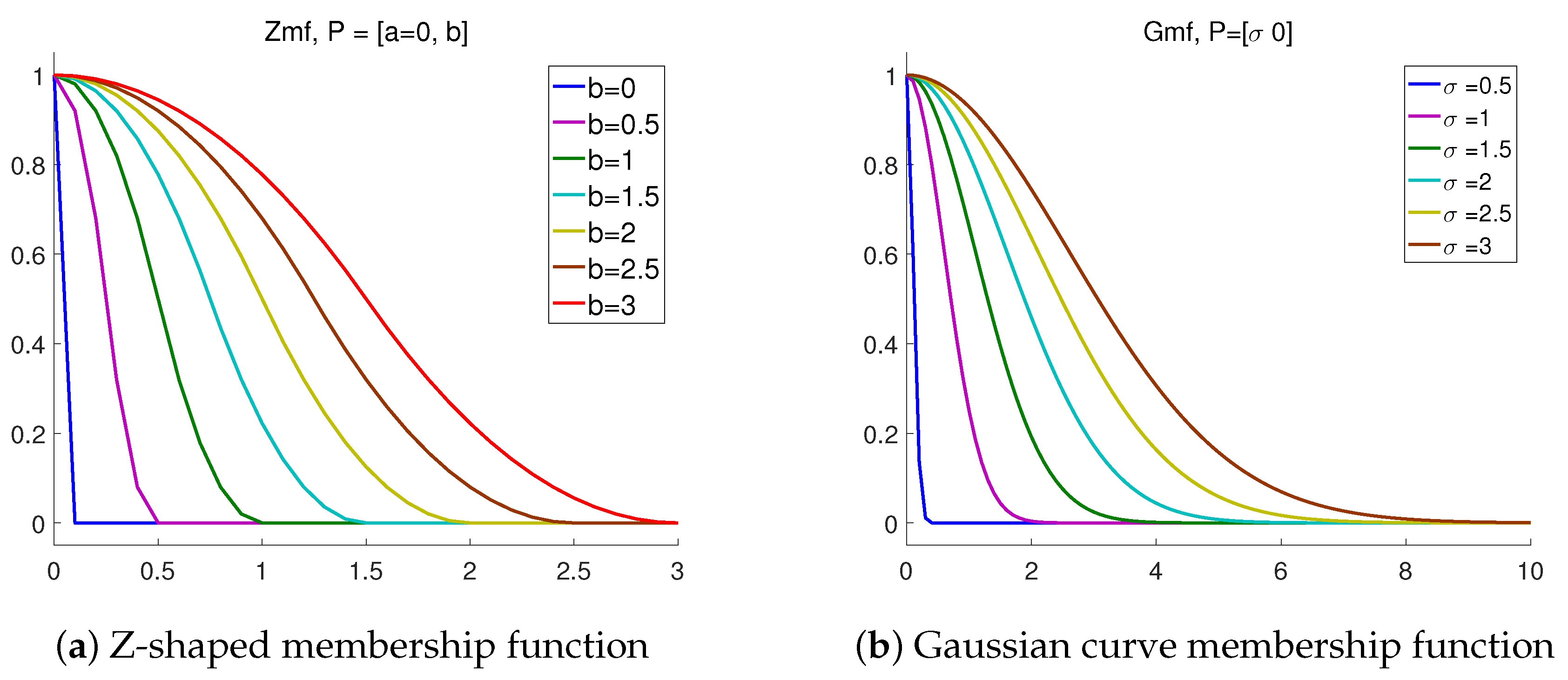
  • Any fuzzy membership function (like the Gaussian one used in the following) can be used in calculating MFSampEn: μ ( d i j , r ) = exp ( ( d i j ) 2 2 r 2 ) .

2.1. The Multivariate Fuzzy Sample Entropy

To calculate multivariate fuzzy sample entropy (MFSampEn), recall from multivariate embedding theory [26], that for a p-variate time series { x k , i } i = 1 N , k = 1 , 2 , , p , observed through p measurement functions h k ( y i ) , the multivariate embedded reconstruction is based on the composite delay vector
X m ( i ) = [ x 1 , i , x 1 , i + τ 1 , , x 1 , i + ( m 1 1 ) τ 1 , x 2 , i , x 2 , i + τ 2 , , x 2 , i + ( m 2 1 ) τ 2 , , x p , i , x p , i + τ p , , x p , i + ( m p 1 ) τ p ] ,
where M = [ m 1 , m 2 , , m p ] R p is the embedding vector, τ = [ τ 1 , τ 2 , , τ p ] the time lag vector, and the composite delay vector X m ( i ) R m (where m = k = 1 p m k ). It is also important to note that if some channels of a multivariate data have different amplitude range, the distances calculated on such composite delay vectors could be biased towards the variates with largest ranges. On the other hand, the different data channels may also be of different nature and measured in different units. To this end, in our proposed formulation of multivariate fuzzy sample entropy, we first normalize the multivariate data (with zero mean and unit variance). This allows us to cater for multimodal signals obtained from different sources.
For a p-variate time series { x k , i } i = 1 N , k = 1 , 2 , , p , we introduce MFSampEn through the following procedure:
  • Form ( N n ) composite delay vectors X m ( i ) R m , where i = 1 , 2 , , N n and n = max { M } × max { τ } ;
  • For each delay vector, remove the local mean: X m ( i ) = [ x ( i ) x 0 ( i ) , x ( i + 1 ) x 0 ( i ) , , x ( i + m 1 ) x 0 ( i ) ] where x 0 ( i ) = 1 m j = 0 m 1 x ( i + j ) ;
  • Define the distance between any two composite delay vectors X m ( i ) and X m ( j ) as the maximum norm [27], that is, d i j m = d [ X m ( i ) , X m ( j ) ] = max l = 1 , , m { | x ( i + l 1 ) x ( j + l 1 ) | } ;
  • For a given composite delay vector X m ( i ) and a tolerance r, calculate the similarity degree D i j m to other vector X m ( j ) through a fuzzy membership function μ ( d i j m , r ) , i.e., D i j m ( r ) = μ ( d i j m , r ) . Then, define the function
    B m ( r ) = 1 N n i = 1 N n 1 N n 1 j = 1 , j i N n 1 D i j m ;
  • Extend the dimensionality of the multivariate delay vector in Step 1 from m to ( m + 1 ) . This can be performed in p different ways, as from a space defined by the embedding vector M = [ m 1 , m 2 , , m k , , m p ] the system can evolve to any space for which the embedding vector is [ m 1 , m 2 , , m k + 1 , , m p ] ( k = 1 , 2 , , p ). Thus, a total of p × ( N n ) vectors X m + 1 ( i ) in R m + 1 are obtained, where X m + 1 ( i ) denotes any embedded vector upon increasing the embedding dimension from m k to ( m k + 1 ) for a specific variable k. In the process, the embedding dimension of the other data channels is kept unchanged, so that the overall embedding dimension of the system undergoes the change from m to ( m + 1 ) ;
  • For a given X m + 1 ( i ) , calculate the similarity degree D i j m + 1 to another vector X m + 1 ( j ) through a fuzzy membership function μ ( d i j m + 1 , r ) , i.e., D i j m + 1 ( r ) = μ ( d i j m + 1 , r ) . Then, define the function
    B m + 1 ( r ) = 1 p ( N n ) i = 1 p ( N n ) 1 p ( N n ) 1 × j = 1 , j i p ( N n ) 1 D i j m + 1
  • In this way, B m ( r ) represents the probability that any two composite delay vectors are similar in the dimension m, whereas B m + 1 ( r ) is the probability that any two composite delay vectors will be similar in the dimension ( m + 1 ) .
  • Finally, for a tolerance level r, MFSampEn is calculated as the negative of a natural logarithm of the conditional probability that two composite delay vectors close to each other in an m-dimensional space will also be close to each other when the dimensionality is increased by one, and can be estimated by the statistic
    M F S a m p E n ( M , τ , r , N ) = l n B m + 1 ( r ) B m ( r )
The multivariate multiscale fuzzy entropy (MMFE) plots, that is, multivariate fuzzy sample entropy evaluated as a function of the scale factor, are next used to assess the relative complexity of normalized multi-channel temporal data.

2.2. Fuzzy Membership Function

Any fuzzy membership function which has smooth transitional boundaries can be used to calculate the degree of similarity between any two delay vectors. In this study, two fuzzy membership functions known as the Gaussian and Z-shaped membership function are considered to examine the degrees of similarity as they are known to yield consistent entropy values when applied to a variety of datasets [25]. It is possible to apply other fuzzy membership functions with the MMFE, however, they would produce only slightly different results from the two functions which we have selected.
The Z-shaped membership function (Zmf) is a spline-based function of x and is so named because of its Z-shape. The parameters a and b determine the extremes of the sloped portion of the curve, given by:
f ( x ; a , b ) = 1 , x a 1 2 x a b a 2 , a x a + b 2 2 x b b a 2 , a + b 2 x b 0 , x b
The second fuzzy function considered, the Gaussian curve membership function (Gmf), is a symmetric Gaussian function which depends on two parameters, σ and c, and is given by:
f ( x ; σ , c ) = exp ( ( x c ) 2 2 σ 2 )
Figure 1 illustrates the Z-shaped membership function with a = 0 and for different values of b (in Figure 1a) and the Gaussian curve membership function with c = 0 and for different values of σ (in Figure 1b). Both the functions are suitable for calculating MFSampEn and are considered in this paper. From Figure 1, observe that the fuzzy function changes continuously and gradually, unlike the Heaviside function used in SampEn and MSampEn which changes abruptly. It should be noted that although the qualitative behavior of both the fuzzy functions are relatively similar, numerically Z-shaped function yields higher entropy estimates than the Gaussian function. This is due to the fact that the integrals under the respective curves are rather different for the considered setting ( b = s i g m a = r ) and, thus, the weights (according to the fuzzy function) associated with all paired composite delay vectors are essentially different.

3. Validation on Synthetic Data

The multivariate MSE analysis has shown [19,20] that for multi-channel random white noise (uncorrelated), the multivariate sample entropy values decrease monotonically with scale, whereas for multi-channel 1 / f noise (long-range correlated) multivariate sample entropy remains more or less constant over multiple time scales. This indicates that the multivariate 1 / f noise is structurally more complex than uncorrelated multivariate random signals.
To illustrate the corresponding behaviour for the multivariate multiscale fuzzy entropy (MMFE), we generated two trivariate time series, for which in one time series, all the data channels were realizations of mutually independent white noise and in other series all the data channels were realizations of mutually independent 1 / f noise. Figure 2 shows both the MMSE and MMFE curves for the cases considered. The analysis in Figure 2 therefore confirms that the multivariate 1 / f noise exhibits long-range correlations and thus has higher overall complexity than the multivariate random white noise and that the multivariate fuzzy sample entropy is more consistent and accurate at larger scales compared to MMSE, as indicated by smaller error bars.

3.1. Effect of Data Length on Multivariate Fuzzy Sample Entropy

It has been empirically found in [18,20] that MSampEn estimates are consistent for data length N 300 and are sufficient for robust estimation. To assess the sensitivity of the proposed multivariate fuzzy sample entropy (MFSampEn) to the data length parameter, we evaluated MFSampEn of a 3-channel white as well as 1 / f noise as a function of sample size N, where for each channel the embedding dimension m k = 2 and the threshold r = 0.15 . Figure 3 shows that for both the white and 1 / f 3-channel noise, MFSampEn estimates were consistent for data lengths which were by far shorter than those required by MSampEn. Note also that the MFSampEn estimates are more robust for shorter data lengths than MSampEn estimates, as seen from the error bars in Figure 3. The MMSE (MSE) calculates MSampEn (SampEn) for different scales generated by the coarse-graining process and the length of each coarse-grained time series is equal to the length of the original time series divided by the scale factor, ϵ. The coarse graining procedure of the standard MMSE approach thus imposes the constraint that the highest scale should have enough data points (at least 300 points) to be able to calculate a valid entropy estimate. This limits the applicability of coarse graining based MMSE for short data. Our proposed MMFE overcomes this limitation and is applicable to short data, even as small as 30 samples, using Gaussian curve fuzzy membership function, as shown in Figure 3a.

3.2. Sensitivity to the Embedding Dimension

Physically, for the standard univariate sample entropy, the increase in sample entropy values with an increase in embedding dimension m is due to progressively fewer delay vectors to compare as m increases. On the contrary, for MSampEn the increase in m does not reduce the number of the available delay vectors, as the composite multivariate embedded vectors are constructed in parallel, as pointed out in [18]. Nevertheless, a valid MSampEn estimate at higher m k requires a progressively higher number of samples. On the other hand, for higher m k , MFSampEn can be estimated with comparatively lower number of samples. This phenomenon is shown in Figure 4 which presents an MFSampEn/MSampEn vs. m k plot for a 3-channel white and 1 / f noise with 1000 points in each channel. Figure 4 illustrates that the result for MFSampEn is more consistent, as white noise remains higher in complexity than 1 / f noise at the lowest scale for the embedding dimension up to m k = 4 , for a Gaussian membership function (Figure 4a), and for the embedding dimension up to m k = 3 for Z-shaped membership function(Figure 4b). On the other hand, MSampEn estimates are consistent only for the embedding dimension of up to m k = 2 for 1000 samples and undefined for higher m k values. For a large m k , the length of the time series required for a valid entropy estimate would be higher, and therefore for practical purposes, m k is selected in the range of 1–3 in the literature.

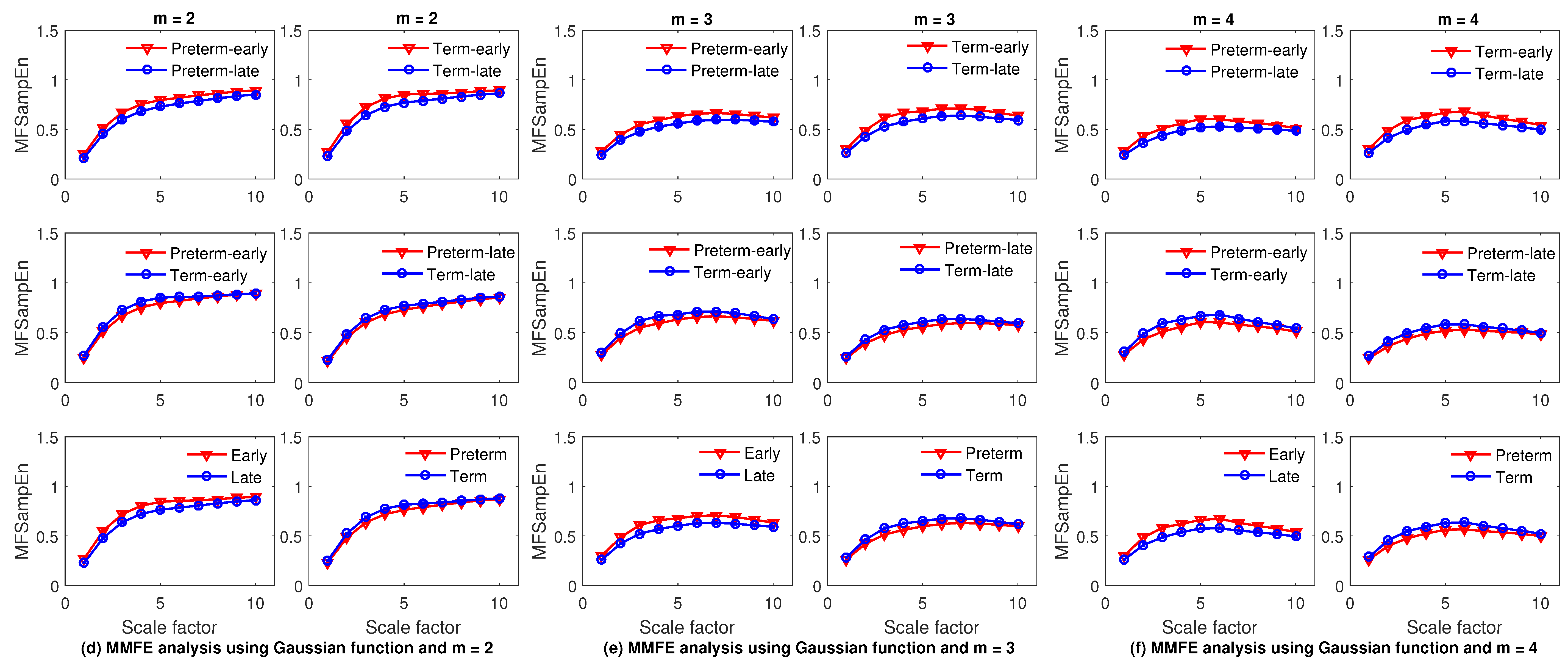
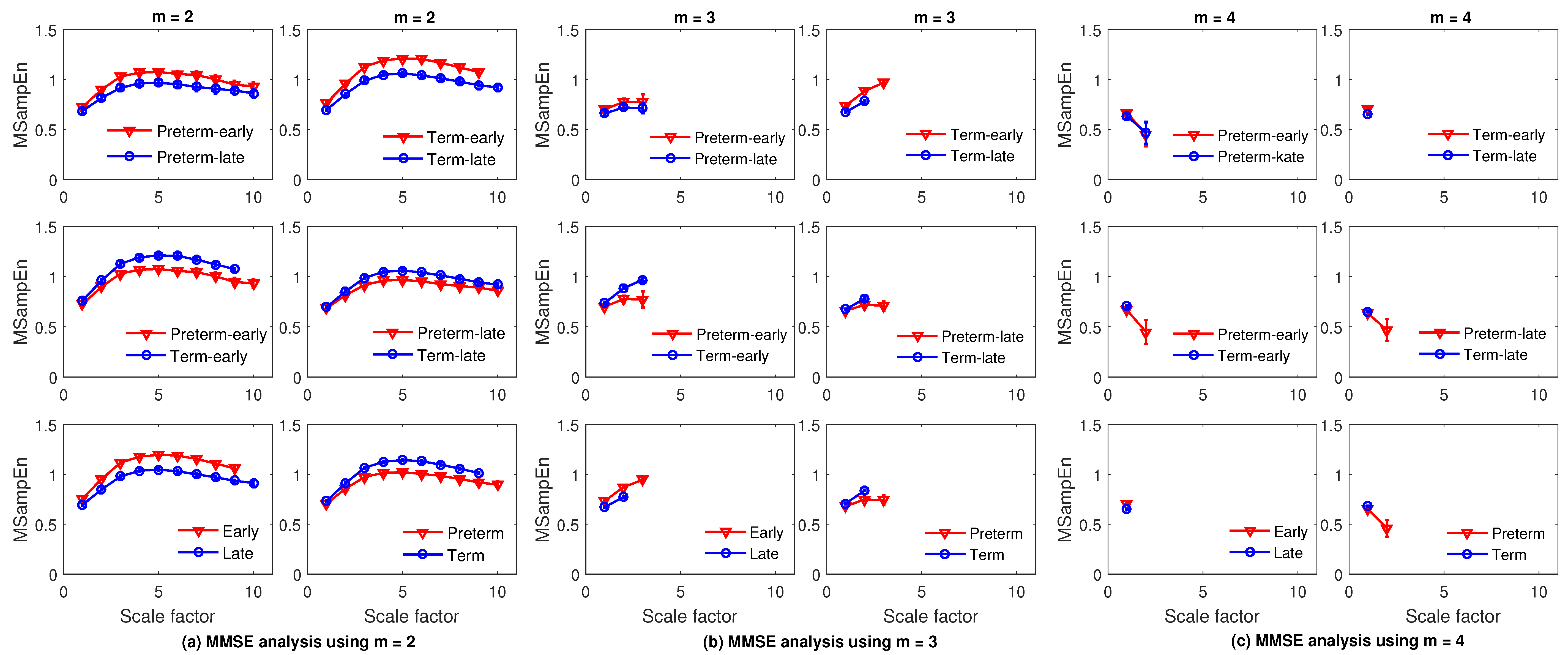
4. Applications to Uterine EMG Signal Chracterization

Uterine electromyogram (UEMG) or Electrohysterogram (EHG) represents the spontaneous myometrial bioelectrical activity in the form of intermittent bursts of action potentials that triggers the mechanical contraction of the uterus [28]. The UEMG is gaining popularity as promising and powerful new tool for characterizing the parturition process due to its non-invasive and economical nature.
The process of parturition involves a relatively long conditioning (preparatory) phase, followed by a short active labor [29]. During the preparatory phase, excitability of the myometrial cells increases due to the changes in transduction mechanisms and synthesis of several new proteins, including ion channels and receptors for uterotonins. As the delivery approaches, cell-to-cell gap junctions form and electrical coupling between myometrial cells increase, thus creating the electrical syncytium required for effective contractions. Eventually, the preparatory process becomes irreversible and leads to active labor. In labor, this bioelectrical activity becomes more synchronous resulting towards the complete dilation of the cervix and expulsion (delivery) of the fetus [28,30].
Normally, pregnancy in humans lasts about 40 weeks. According to the World Health Organization (WHO) and the International Federation of Gynecology and Obstetrics (FIGO), delivery of babies born alive before 37 weeks of gestation is considered preterm delivery/birth whereas term delivery implies birth between 37 to 42 weeks [31]. Preterm birth is a global problem. It occurs in high, low, and middle-income countries. About 15 million babies are born preterm each year, that is, more than 1 in 10 babies worldwide and this number is rising [32]. Preterm birth complications are the leading cause of death among children under 5 years of age, responsible for nearly 1 million deaths in 2013 [32]. In addition to its significant contribution to neonatal mortality, many survivors of preterm birth face a lifetime of disability, including learning disabilities, visual and hearing problems, as well as long-term physical health issues with a higher risk of non-communicable disease [32,33,34]. These certainly add significant costs to the economy as well as throw a heavy burden on families, society and the health system [35].
Although numerous risk factors of preterm birth have been identified, such as diabetes, conization, hypertension, uterine abnormalities, preterm premature rupture of membranes (PPROM), previous preterm delivery, multiple births, recurrent antepartum haemorrhage, illnesses and infections, any invasive procedure or surgery, underweight or obesity, ethnicity, alcohol and drug use, smoking, folic acid deficiency, a positive fibronectin test and others, the exact causes of many preterm births are still unresolved [35,36]. Current methods of preterm birth prediction based on calculating the aforementioned risk factors alone are unreliable and uncertain [37]. However, predicting preterm birth and diagnosing preterm labor obviously have important consequences for babies, families, societies and the economy. Effective prediction of preterm births could contribute to improving prevention, through appropriate medical and lifestyle interventions [36]. Nevertheless, none of the currently available clinical methods can distinguish reliably between true and false term and preterm labor. On the other hand, evidence from many studies suggest that UEMG recordings can diagnose true labor more accurately than any other method used today [30]. As a result, UEMG provides a strong basis for objective prediction and diagnosis of preterm birth [36].
So far, various signal processing techniques have been used to analyze UEMG signals. To understand the underlying parturition mechanisms of the uterus, traditionally linear analysis methods based on either time domain or transform domain parameters are used. As the uterus is an extremely complex biological structure consisting billions of intricately interconnected myometrial cells whose responses are non-linear, it may be considered as a complex, non-linear dynamic system [38]. Besides, it is widely accepted that the underlying physiological mechanisms in all biological systems are non-linear processes [39,40,41]. As a result, nonlinear signal processing techniques are also used to characterize UEMG signals lately. G. Fele-Zorz et al. applied several linear and nonlinear methods to separate term and preterm deliveries and showed better discrimination results with nonlinear methods [38]. Fergus et al. [36] showed an improvement over existing studies using both linear and non-linear features extracted from the UEMG recording within a supervised machine-learning paradigm. Using SampEn and adaptive autoregressive (AAR) method for feature extraction and support vector machine classifier for classification, Smrdel et al. [37] concluded that the SampEn better reflected the physiological mechanisms of the term and preterm UEMG records which were confirmed by the better classification accuracy achieved. Improved prediction of preterm delivery by using empirical mode decomposition, a novel nonlinear time-frequency approach was reported in [35].
In this paper, we used two nonlinear, multiscale and multivariate methods, namely the multivariate multiscale entropy (MMSE) and multivariate multiscale fuzzy entropy (MMFE), to characterize and extract features from the UEMG records. The so extracted features were classified within a supervised machine learning paradigm, with a view to demonstrate the superiority of MMFE over MMSE for short data lengths.

4.1. TPEHG Database

The Electrohysterogram records (uterine EMG records) used in this study are included in the Term-Preterm Electrohysterogram Database (TPEHG DB) which is publicly available from PhysioNet [42]. The records were obtained during regular check-ups either around the 22nd week of gestation or around the 32nd week of gestation. The database contains 300 uterine EMG records from 300 pregnancies (one record per pregnancy) of which:
  • 262 records were obtained during pregnancies where delivery was on term (duration of gestation at delivery >37 weeks):
    143 records were obtained before the 26th week of gestation (Term-early);
    119 were obtained later during pregnancy, during or after the 26th week of gestation (Term-Late);
  • 38 records were obtained during pregnancies which ended prematurely (pregnancy duration ≤37 weeks), of which:
    19 records were obtained before the 26th week of gestation (Preterm-early);
    19 records were obtained during or after the 26th week of gestation (Preterm-late).
Each record is composed of three channels, recorded from 4 electrodes, sampled at 20 Hz and of 30 min in duration. The first electrode (E1) was placed 3.5 cm to the left and 3.5 cm above the navel; the second electrode (E2) was placed 3.5 cm to the right and 3.5 cm above the navel; the third electrode (E3) was placed 3.5 cm to the right and 3.5 cm below the navel; and the fourth electrode (E4) was placed 3.5 cm to the left and 3.5 cm below the navel. The differences in the electrical potentials of the electrodes were recorded, producing 3 data channels: S1 = E2 − E1 (first channel); S2 = E2 − E3 (second channel); and S3 = E4 − E3 (third channel).
Next, each signal was digitally filtered using three different 4-pole digital Butterworth filters with a double-pass filtering scheme to ensure zero phase shift. A detailed discussion about the database is given in [38]. We have chosen three different m values, that is m = 2, 3, and 4 for MMFE/MMSE analysis. Previous research has suggested that the UEMG frequency band from 0.3 to 3 Hz contains the most useful information and leaves out most artefacts due to respiration, motion and cardiac signals [35,36,38]. Therefore, only the filtered data with cut-off frequency 0.3–3Hz was used in this study. In all the cases, r was taken as 0.15 times the total variation of the 3-channel UEMG signal.

4.2. Feature Extraction Using MMFE and MMSE

Due to the transients at the beginnings and ends of the filtered signals, a 1.5-min portion of the signals from the beginnings and ends of the 30 min UEMG records were not considered, as suggested in [38]. Thus, the middle 27 min of each signal of the UEMG records were considered. To show the better suitability of the MFSampEn over MSampEn for short record lengths, each 27-min duration records were further divided into 27 one-min epochs. Then both MMFE and MMSE analyses were performed on each one-min epoch (which had 60 × 20 = 1200 samples) and afterwards averaged over the 27 epochs to produce the MMFE or MMSE curves for each record. In this multiscale study, we considered 10 scales for each epoch, so that the coarse graining process of MMFE/MMSE analysis yielded only 120 samples at the highest scale, which however was sufficient for MFSampEn calculation. These MSampEn or MFSampEn values calculated on 10 different coarse-graining scales were used as features in classification stage.
Figure 5 shows the multivariate complexity profiles of the three channel UEMG recordings determined by MMSE (Figure 5a–c), MMFE with Gaussian curve fuzzy membership function (Figure 5d–f) and MMFE using Z-shaped fuzzy membership function (Figure 5g–i). Initially, we calculated those profiles for the embedding dimension m = 2 (Figure 5a,d,g). In each figure, six different scenarios were analyzed. The top-left panel shows the complexity curve for preterm subjects recorded early (before 26 weeks of gestation) vs. those recorded late (after 26 weeks of gestation). The top-right panel depicts similar comparison (early vs. late recordings) but now for termed subjects. The complexity of the Preterm-early versus Term-early is illustrated in the middle-left panel, and for the Preterm-late versus Term-late is shown in the middle-right panel. Finally, the bottom-left panel compares all the early recordings vs. late recordings, irrespective of preterm or term birth, while the bottom-right panel compares the complexity profiles between preterm and term births, irrespective of their recording times. Both complexity estimates (MSampEn and MFSampEn) could discriminate well between different cases in each scenario.
Observe significant differences between the UEMG signals recorded early and late (top-left, top-right and bottom-left panel of Figure 5a,d,g). In other words, as the time of gestation progresses, the MSampEn/MFSampEn values for both term and pre-term delivery records drop, indicating higher predictability or less complexity of the signals as the delivery approaches [43]. On the other hand, the MSampEn/MFSampEn values are lower for pre-term delivery records (middle-left, middle-right and bottom-right panel of Figure 5a,d,g) regardless of the gestation duration at the time of recording, which confirms that the preterm delivery records are less complex or more predictable than the signals of term delivery records. In addition, in all the cases, the separation is better if we consider the multiscale complexity curves rather than the measures in scale 1 only. This also confirms that the original signal not only contains information at the smallest scale but also reveals new information at all scales. This makes it possible to even classify between term and preterm labor earlier in pregnancies.
To demonstrate the suitability of the proposed MMFE method over the MMSE method for short time series, we also calculated the complexity profiles with the embedding dimension m = 3 (Figure 5b,e,h) and m = 4 (Figure 5c,f,i) for both methods. Figure 5b,c confirm that for higher embedding dimensions, there were not enough sample points to calculate MSampEn at higher scales whereas we could calculate MFSampEn with a Gaussian fuzzy membership function for scales up to 10, as shown in Figure 5e,f. However, although we had enough sample points to calculate MFSampEn up to scale 10 with a Z-shaped fuzzy membership function for embedding dimension m = 3 (Figure 5h), we could calculate only up to scale 4 for embedding dimension m = 4 (Figure 5i). This corresponds to the simulation result in Figure 4b.

4.3. Approach for Imbalanced Learning

As the TPEHG database used in this study was unbalanced, comprising 38 true positives (minority class, preterm delivery) and 262 true negatives (majority class, term delivery), their prior probabilities were not equal. As a result, classifiers would be more sensitive in detecting the majority class than the minority one which could lead to biased classification. There are two approaches to imbalanced learning: over-sampling and under-sampling. The under-sampling in this case would remove 224 records from the majority class to make both the classes balanced, leaving us with a small dataset of only 38 records in each class. On the other hand, the over-sampling would generate additional synthetic data in the minority class to make the number of records equal to the majority one. Generally, the over-sampling approach is preferred due to no data loss and accurate results in terms of the area under the ROC (receiver operator curve ) curve (AUC) [44].
In this study, to solve the class skew problem, the Adaptive Synthetic Sampling (ADASYN) [44,45] technique was used. The purpose of the ADASYN technique is to improve class balance by synthetically creating new examples from the minority class via linear interpolation between existing minority class examples. This approach is known as the SMOTE method (Synthetic Minority Oversampling TEchnique) [44,46]. The ADASYN is an extension of SMOTE, which creates more examples in the vicinity of the boundary between the two classes than in the interior of the minority class.

4.4. Classifiers Used

Within the supervised machine learning paradigm, a total of 23 classifiers were tested which fall under six broad classifier categories, namely, decision trees, discriminant analysis, logistic regression, support vector machines (SVM), nearest neighbour (NN) classifiers and ensemble classifiers. The decision tree classifier is a simple and widely used non-parametric classification technique where the goal is to create a model that predicts the value of a target variable by learning simple decision rules inferred from the data features. Three subtypes, namely, simple, medium and complex tree were used in this category. The discriminant analysis assumes that different classes generate data based on different Gaussian distributions. Both linear and quadratic discriminants were tested in this category. The logistic regression is a popular simple classification algorithm which models the class probabilities as a function of the linear combination of predictors. An SVM classifies data by finding the best hyperplane (the one with the largest margin between the two classes) that separates data points of different classes mapping into a higher dimensional space through some kernel function. In this category, linear, quadratic, cubic, fine Gaussian, medium Gaussian and coarse Gaussian SVM classifiers were used. Nearest neighbour (NN) classifiers are also a class of non-parametric methods which classify objects based on closest training examples in the feature space. In this category, six classifiers were chosen, namely, fine K-nearest neighbour (KNN), medium KNN, coarse KNN, cosine KNN, cubic KNN and weighted KNN. Ensemble classifiers combine results from many weak learners into one high-quality ensemble predictor. Boosted trees, Bagged trees, Subspace discriminant, Subspace KNN and RUSBoost trees were tested in this category. The classification learner App of the MATLAB program (R2016a) was used to implement all the above classifiers. The default values of the different parameters were chosen for the classifiers. Besides, a 10-fold cross-validation was employed where the original dataset was first divided into ten equal subsets and then one subset was tested using the classifier which was trained on the remaining nine subsets. This procedure was repeated until every subset had been tested. The overall accuracy of the classifier was then calculated as the average of the ten classification runs. Moreover, sensitivity (which refers the proportion of true positives or preterm records) and specificity (which refers the proportion of true negatives or term records) which measure the predictive capabilities of binary classifiers, were also computed. In our study, sensitivities were given higher priority than specificities as predicting preterm delivery is more important than misclassifying term delivery. Finally, the receiver operator curve (ROC), which is a standard technique to evaluate binary classifier performance, was calculated and the area under the curve (AUC) was determined for each classification method. The greater the AUC value, the greater the discrimination potential of a classifier [44,46].

4.5. Results and Discussion

Table 1 summarizes the classifier performances on the TPEHG database. From Figure 5a, it can be seen that at scale 10, the MSampEn value for early recordings from the term pregnancies are not defined. From Figure 5b, observe that for ϵ > 3 , MSampEn for this study was undefined. Similarly, from Figure 5c, it can be seen that for ϵ > 1 , MSampEn for this study was also undefined. As a result, only classification performances for the parameters which were defined were reported in Table 1. Moreover, to make a fair comparison between MMSE and MMFE in Table 1, only first 9 components were taken after applying principal component analysis(PCA) on the 10-element feature vectors which explained 100% variance in total. Among the categories of early recordings, late recordings and both categories combined, the highest classification accuracy (CA) is shown in bold. In the early recordings category, the fine Gaussian SVM yielded 95.4% classification accuracy in detecting the term and preterm recordings when the feature vectors were computed using MMFE with a Z curve membership function and embedding parameter m = 2 . This was 2.4% higher than the classification accuracy calculated using MMSE features. For the late recordings category, the highest 94.4% CA was achieved with the same classifier when the feature vectors were calculated using MMFE with the Gaussian membership function and the embedding parameter m = 2 . This was 6% higher than that calculated using MMSE features. When both early and late recordings were combined, the same classifier (fine Gaussian SVM) with MMFE features yielded the highest 94.9% CA with the embedding parameter m = 2 , a 3% increase compared to the CA calculated with the MMSE features. Moreover, the best AUC values were also observed for MMFE features.
We also examined whether the number of features had any impact on the classification performance. To that cause, after PCA, for further classification, we only took the first 6 components of the feature vector, which explained 99.5% variance in total. The result is shown in Table 2, which depicts that although CA decreased in most cases (but remained higher for MMFE features), the difference between the CA calculated using MMFE features and that using MMSE features was increased. This confirms that MMFE features performed better in classification when the number of features was smaller.
In comparison with the previous studies using UEMG signals from the same TPEHG database, our study produced significantly better results than those reported in [35,36,37]. Using four features (root mean squares, peak frequency, median frequency, sample entropy) and eleven items of additional clinical information (in total, a 15-element feature vector), the best classification accuracy (regardless of the time of recording) reported in [36] was 92%, with a 0.95% AUC value. In [35], the highest AUC value of 98.6% was obtained when an AdaBoost classifier with a 180-element feature vector extracted from EMD (empirical mode decomposition) based approach was used. Considering sample entropy estimation from three channels separately and additional clinical information (yielding 14 element feature vector per record), an 87% classification accuracy was achieved using SVM classifier in [37]. However, using only 9 element feature vectors extracted from MMFE analysis, we achieved the highest AUC of 99% with the classification accuracy of 95% in classifying between the term and preterm records, regardless of the time of recording. This validates the proposed MMFE method, and demonstrates its superiority over MMSE.

5. Conclusions

We have extended the recently introduced multivariate multiscale entropy (MMSE) method using fuzzy membership functions, in order to cater for short time recordings. The so introduced multivariate multiscale fuzzy entropy (MMFE) algorithm has been validated on the classification of uterine EMG recordings and has shown that differences in the UEMG signals exist in terms of the gestational age, which can be utilized to predict preterm delivery. Overall, our study has suggested that the MMFE analysis can characterize the physiology of parturition well and can also provide a better way of discriminating women at risk of preterm delivery than the existing methods.

Acknowledgments

Mosabber U. Ahmed is a Commonwealth Academic Fellow, funded by the UK government. The work of Danilo P. Mandic was supported by EPSRC, grant EP/K025643/1. Sudhin Thayyil was supported by the Biomedical Research Centre, Imperial College London, grant P51286.

Author Contributions

Mosabber U. Ahmed conceived the method, and Mosabber U. Ahmed, Theerasak Chanwimalueang, and Danilo P. Mandic designed the method. Mosabber U. Ahmed and Sudhin Thayyil established the UEMG analysis framework. Mosabber U. Ahmed, Theerasak Chanwimalueang, and Danilo P. Mandic analyzed the data; Sudhin Thayyil analysed the findings in the medical context. All authors contributed to writing of the manuscript and commented on the manuscript at all stages. All authors have read and approved the final manuscript.

Conflicts of Interest

The authors declare no conflict of interest.

References

  1. Grassberger, P. Toward a quantitative theory of self-generated complexity. Int. J. Theor. Phys. 1986, 25, 907–938. [Google Scholar] [CrossRef]
  2. Gell-Mann, M. Let’s call it plectics. Complexity 1995, 1, 3. [Google Scholar] [CrossRef]
  3. Goldenfeld, N.; Kadanoff, L.P. Simple Lessons from Complexity. Science 1999, 284, 87–89. [Google Scholar] [CrossRef] [PubMed]
  4. Foote, R. Mathematics and Complex Systems. Science 2007, 318, 410–412. [Google Scholar] [CrossRef] [PubMed]
  5. Ladyman, J.; Lambert, J.; Wiesner, K. What is a complex system? Eur. J. Philos. Sci. 2013, 3, 33–67. [Google Scholar] [CrossRef]
  6. Manson, S.M. Simplifying complexity: A review of complexity theory. Geoforum 2001, 32, 405–414. [Google Scholar] [CrossRef]
  7. Editorial. No man is an island. Nat. Phys. 2009, 5. [Google Scholar] [CrossRef]
  8. Pincus, S.M. Approximate entropy as a measure of system complexity. Proc. Natl. Acad. Sci. USA 1991, 88, 2297–2301. [Google Scholar] [CrossRef] [PubMed]
  9. Richman, J.S.; Moorman, J.R. Physiological time-series analysis using approximate entropy and sample entropy. AJP Heart Circ. Physiol. 2000, 278, 2039–2049. [Google Scholar]
  10. Costa, M.; Goldberger, A.L.; Peng, C.K. Multiscale entropy analysis of complex physiologic time series. Phys. Rev. Lett. 2002, 89, 068102. [Google Scholar] [CrossRef] [PubMed]
  11. Costa, M.; Goldberger, A.L.; Peng, C.K. Multiscale entropy analysis of biological signals. Phys. Rev. E 2005, 71, 021906. [Google Scholar] [CrossRef] [PubMed]
  12. Hornero, R.; Abásolo, D.; Escudero, J.; Gomez, C. Nonlinear analysis of electroencephalogram and magnetoencephalogram recordings in patients with Alzheimer’s disease. Phil. Trans. R. Soc. A 2009, 367, 317–336. [Google Scholar] [CrossRef] [PubMed] [Green Version]
  13. Costa, M.; Peng, C.K.; Goldberger, A.L.; Hausdorff, J.M. Multiscale entropy analysis of human gait dynamics. Physica A 2003, 330, 53–60. [Google Scholar] [CrossRef]
  14. Takahashi, T.; Cho, R.Y.; Murata, T.; Mizuno, T.; Kikuchi, M.; Mizukami, K.; Kosaka, H.; Takahashi, K.; Wada, Y. Age-related variation in EEG complexity to photic stimulation: A multiscale entropy analysis. Clin. Neurophysiol. 2009, 120, 476–483. [Google Scholar] [CrossRef] [PubMed]
  15. Costa, M.; Ghiran, I.; Peng, C.K.; Nicholson-Weller, A.; Goldberger, A.L. Complex dynamics of human red blood cell flickering: Alterations with in vivo aging. Phys. Rev. E 2008, 78, 020901. [Google Scholar] [CrossRef] [PubMed]
  16. Humeau-Heurtier, A. The Multiscale Entropy Algorithm and Its Variants: A Review. Entropy 2015, 17, 3110–3123. [Google Scholar] [CrossRef] [Green Version]
  17. Valencia, J.; Porta, A.; Vallverdu, M.; Claria, F.; Baranowski, R.; Orlowska-Baranowska, E.; Caminal, P. Refined Multiscale Entropy: Application to 24-h Holter Recordings of Heart Period Variability in Healthy and Aortic Stenosis Subjects. IEEE Trans. Biomed. Eng. 2009, 56, 2202–2213. [Google Scholar] [CrossRef] [PubMed]
  18. Ahmed, M.; Rehman, N.; Looney, D.; Rutkowski, T.; Mandic, D. Dynamical complexity of human responses: a multivariate data-adaptive framework. Bull. Pol. Acad. Sci. Tech. Sci. 2012, 60, 433–445. [Google Scholar] [CrossRef]
  19. Ahmed, M.U.; Mandic, D.P. Multivariate multiscale entropy: A tool for complexity analysis of multichannel data. Phys. Rev. E 2011, 84, 061918. [Google Scholar] [CrossRef] [PubMed]
  20. Ahmed, M.U.; Mandic, D.P. Multivariate Multiscale Entropy Analysis. IEEE Signal Process. Lett. 2012, 19, 91–94. [Google Scholar] [CrossRef]
  21. Wu, S.D.; Wu, C.W.; Lin, S.G.; Wang, C.C.; Lee, K.Y. Time Series Analysis Using Composite Multiscale Entropy. Entropy 2013, 15, 1069–1084. [Google Scholar] [CrossRef]
  22. Wu, S.D.; Wu, C.W.; Lin, S.G.; Lee, K.Y.; Peng, C.K. Analysis of complex time series using refined composite multiscale entropy. Phys. Lett. A 2014, 378, 1369–1374. [Google Scholar] [CrossRef]
  23. Humeau-Heurtier, A. Multivariate refined composite multiscale entropy analysis. Phys. Lett. A 2016, 380, 1426–1431. [Google Scholar] [CrossRef] [Green Version]
  24. Zadeh, L. Fuzzy sets. Inf. Control 1965, 8, 338–353. [Google Scholar] [CrossRef]
  25. Chen, W.; Wang, Z.; Xie, H.; Yu, W. Characterization of Surface EMG Signal Based on Fuzzy Entropy. IEEE Trans. Neural Syst. Rehabil. Eng. 2007, 15, 266–272. [Google Scholar] [CrossRef] [PubMed]
  26. Cao, L.; Mees, A.; Judd, K. Dynamics from multivariate time series. Physica D 1998, 121, 75–88. [Google Scholar] [CrossRef]
  27. Grassberger, P.; Schreiber, T.; Schaffrath, C. Nonlinear time sequence analysis. Int. J. Bifurc. Chaos 1991, 1, 521–547. [Google Scholar] [CrossRef]
  28. Vinken, M.P.G.C.; Rabotti, C.; Mischi, M.; Oei, S.G. Accuracy of Frequency-Related Parameters of the Electrohysterogram for Predicting Preterm Delivery: A Review of the Literature. Obstet. Gynecol. Surv. 2009, 64, 529–541. [Google Scholar] [CrossRef] [PubMed]
  29. Garfield, R.E.; Maner, W.L. Physiology and electrical activity of uterine contractions. Semin. Cell Dev. Biol. 2007, 18, 289–295. [Google Scholar] [CrossRef] [PubMed]
  30. Lucovnik, M.; Kuon, R.J.; Chambliss, L.R.; Maner, W.L.; Shi, S.Q.; Shi, L.; Balducci, J.; Garfield, R.E. Use of uterine electromyography to diagnose term and preterm labor. Acta Obstet. Gynecol. Scand. 2011, 90, 150–157. [Google Scholar] [CrossRef] [PubMed]
  31. Steer, P. The epidemiology of preterm labour. Int J. Obstet. Gynaecol. 2005, 112, 1–3. [Google Scholar] [CrossRef] [PubMed]
  32. Born Too Soon: The Global Action Report on Preterm Birth. Available online: http://www.who.int/pmnch/media/news/2012/201204_borntoosoon-report.pdf (accessed on 20 December 2016).
  33. Rogers, L.K.; Velten, M. Maternal inflammation, growth retardation, and preterm birth: Insights into adult cardiovascular disease. Life Sci. 2011, 89, 417–421. [Google Scholar] [CrossRef] [PubMed]
  34. Harrison, M.S.; Goldenberg, R.L. Global burden of prematurity. Semin. Fetal Neonatal Med. 2016, 21, 74–79. [Google Scholar] [CrossRef] [PubMed]
  35. Ren, P.; Yao, S.; Li, J.; Valdes-Sosa, P.A.; Kendrick, K.M. Improved Prediction of Preterm Delivery Using Empirical Mode Decomposition Analysis of Uterine Electromyography Signals. PLoS ONE 2015, 10, 1–16. [Google Scholar] [CrossRef] [PubMed]
  36. Fergus, P.; Cheung, P.; Hussain, A.; Al-Jumeily, D.; Dobbins, C.; Iram, S. Prediction of Preterm Deliveries from EHG Signals Using Machine Learning. PLoS ONE 2013, 10, e77154. [Google Scholar] [CrossRef] [PubMed]
  37. Smrdel, A.; Jager, F. Separating sets of term and pre-term uterine EMG records. Physiol. Meas. 2015, 36, 341–355. [Google Scholar] [CrossRef] [PubMed]
  38. Fele-Žorž, G.; Kavšek, G.; Novak-Antolič, Ž.; Jager, F. A comparison of various linear and non-linear signal processing techniques to separate uterine EMG records of term and pre-term delivery groups. Med. Biol. Eng. Comput. 2008, 46, 911–922. [Google Scholar] [CrossRef] [PubMed]
  39. Akay, M. Nonlinear Biomedical Signal Processing Vol. II: Dynamic Analysis and Modeling, 1st ed.; Wiley: Hoboken, NJ, USA, 2000. [Google Scholar]
  40. Small, M. Dynamics of Biological Systems, 1st ed.; CRC Press: London, UK, 2011. [Google Scholar]
  41. Strogatz, S.H. Nonlinear Dynamics and Chaos: With Applications to Physics, Biology, Chemistry, and Engineering, 2nd ed.; Westview Press: Cambridge, UK, 2014. [Google Scholar]
  42. Goldberger, A.L.; Amaral, L.A.N.; Glass, L.; Hausdorff, J.M.; Ivanov, P.C.; Mark, R.G.; Mietus, J.E.; Moody, G.B.; Peng, C.K.; Stanley, H.E. PhysioBank, PhysioToolkit, and PhysioNet : Components of a New Research Resource for Complex Physiologic Signals. Circulation 2000, 101, e215–e220. [Google Scholar] [CrossRef] [PubMed]
  43. Di Marco, L.Y.; Di Maria, C.; Tong, W.C.; Taggart, M.J.; Robson, S.C.; Langley, P. Recurring patterns in stationary intervals of abdominal uterine electromyograms during gestation. Med. Biol. Eng. Comput. 2014, 52, 707–716. [Google Scholar] [CrossRef] [PubMed]
  44. He, H.; Garcia, E.A. Learning from Imbalanced Data. IEEE Trans. Knowl. Data Eng. 2009, 21, 1263–1284. [Google Scholar]
  45. He, H.; Bai, Y.; Garcia, E.A.; Li, S. ADASYN: Adaptive synthetic sampling approach for imbalanced learning. In Proceddings of the 2008 IEEE International Joint Conference on Neural Networks, Hong Kong, China, 1–8 June 2008; pp. 1322–1328.
  46. Chawla, N.V.; Bowyer, K.W.; Hall, L.O.; Kegelmeyer, W.P. SMOTE: Synthetic Minority Over-sampling Technique. J. Artif. Int. Res. 2002, 16, 321–357. [Google Scholar]
Figure 1. Two fuzzy membership functions used to calculate the degree of similarity.
Entropy 19 00002 g001
Figure 2. MMFE/MMSE analysis for 3-channel data containing white and 1 / f noise, each with 10,000 data points. The curves represent an average of 20 independent realizations and error bars represent the standard deviation (SD).
Entropy 19 00002 g002
Figure 3. MSampEn/MFSampEn as a function of data length N, for r = 0.15 and m k = 2 in each data channel. Shown are the mean values for 30 simulated trivariate time series containing white and 1 / f noise, while error bars represent the standard deviation (SD). (a) Using Gaussian curve fuzzy membership function with σ = r ; (b) Using Z-shaped fuzzy membership function with b = r .
Entropy 19 00002 g003
Figure 4. MSampEn/MFSampEn as a function of the embedding parameter m k , where for each channel 1000 samples were considered, and r = 0.15 . Shown are the mean values for 30 simulated trivariate time series containing white and 1 / f noise, while error bars correspond to the standard deviation (SD). (a) Using Gaussian curve fuzzy membership function with σ = r ; (b) Using Z-shaped fuzzy membership function with b = r .
Entropy 19 00002 g004
Figure 5. MMSE (ac) and MMFE (di) analyses of the 3-channel UEMG signal with the embedding parameter m = 2, 3 and 4. The curves represent an average of the corresponding populations while the error bars represent the standard deviation (SD).
Entropy 19 00002 g005aEntropy 19 00002 g005bEntropy 19 00002 g005c
Table 1. Summary of classifier performance on TPEHG database. The feature vector was composed of 9 elements. The highest classification accuracy (CA) in each recording category is shown in bold.
Different ParametersBest ClassifierSensitivitySpecificityCAAUC
Early m = 2 , MMSEBagged tree9790930.98
m = 2 , MMFE with Gaussian functionFine Gaussian SVM90100951
m = 2 , MMFE with Z functionFine Gaussian SVM9110095.40.99
m = 3 , MMFE with Gaussian functionFine Gaussian SVM909994.10.99
m = 4 , MMFE with Gaussian functionFine Gaussian SVM8710093.60.99
Late m = 2 , MMSEFine Gaussian SVM789988.50.99
m = 2 , MMFE with Gaussian functionFine Gaussian SVM909994.41
m = 2 , MMFE with Z functionFine Gaussian SVM849991.70.99
m = 3 , MMFE with Gaussian functionQuadratic SVM988993.70.98
m = 4 , MMFE with Gaussian functionFine Gaussian SVM849891.10.98
Early and Late combined m = 2 , MMSEFine Gaussian SVM849991.90.99
m = 2 , MMFE with Gaussian functionFine Gaussian SVM929894.90.99
m = 2 , MMFE with Z functionFine Gaussian SVM909994.30.99
m = 3 , MMFE with Gaussian functionFine Gaussian SVM879792.10.98
m = 4 , MMFE with Gaussian functionFine Gaussian SVM919894.30.98
Table 2. Summary of classifier performance on TPEHG database. The feature vector was composed of 6 elements. The highest classification accuracy (CA) in each recording category is shown in bold.
Different ParametersBest ClassifierSensitivitySpecificityCAAUC
Early m = 2 , MMSEFine Gaussian SVM889591.30.98
m = 2 , MMFE with Gaussian functionFine Gaussian SVM919291.50.98
m = 2 , MMFE with Z functionFine Gaussian SVM899491.80.97
m = 3 , MMFE with Gaussian functionFine Gaussian SVM949996.50.99
m = 4 , MMFE with Gaussian functionFine Gaussian SVM819789.40.98
Late m = 2 , MMSEFine Gaussian SVM769786.40.94
m = 2 , MMFE with Gaussian functionFine Gaussian SVM919392.30.98
m = 2 , MMFE with Z functionFine Gaussian SVM889792.50.98
m = 3 , MMFE with Gaussian functionBagged tree948790.40.96
m = 4 , MMFE with Gaussian functionFine Gaussian SVM889591.60.96
Early and Late combined m = 2 , MMSEFine Gaussian SVM839588.70.95
m = 2 , MMFE with Gaussian functionFine Gaussian SVM919190.90.97
m = 2 , MMFE with Z functionFine Gaussian SVM949292.60.97
m = 3 , MMFE with Gaussian functionFine Gaussian SVM929392.70.98
m = 4 , MMFE with Gaussian functionFine Gaussian SVM939493.50.97

