Multivariate Surprisal Analysis of Gene Expression Levels

Abstract

We consider here multivariate data which we understand as the problem where each data point i is measured for two or more distinct variables. In a typical situation there are many data points i while the range of the different variables is more limited. If there is only one variable then the data can be arranged as a rectangular matrix where i is the index of the rows while the values of the variable label the columns. We begin here with this case, but then proceed to the more general case with special emphasis on two variables when the data can be organized as a tensor. An analysis of such multivariate data by a maximal entropy approach is discussed and illustrated for gene expressions in four different cell types of six different patients. The different genes are indexed by i, and there are 24 (4 by 6) entries for each i. We used an unbiased thermodynamic maximal-entropy based approach (surprisal analysis) to analyze the multivariate transcriptional profiles. The measured microarray experimental data is organized as a tensor array where the two minor orthogonal directions are the different patients and the different cell types. The entries are the transcription levels on a logarithmic scale. We identify a disease signature of prostate cancer and determine the degree of variability between individual patients. Surprisal analysis determined a baseline expression level common for all cells and patients. We identify the transcripts in the baseline as the “housekeeping” genes that insure the cell stability. The baseline and two surprisal patterns satisfactorily recover (99.8%) the multivariate data. The two patterns characterize the individuality of the patients and, to a lesser extent, the commonality of the disease. The immune response was identified as the most significant pathway contributing to the cancer disease pattern. Delineating patient variability is a central issue in personalized diagnostics and it remains to be seen if additional data will confirm the power of multivariate analysis to address this key point. The collapsed limits where the data is compacted into two dimensional arrays are contained within the proposed formalism.

1. Introduction

We derive the extension to multivariate arrays of the thermodynamic-like approach that we have recently proposed for identifying pattern responses in cancerous cell lines and patient data. Our approach is based on information theory and surprisal analysis. It was earlier introduced to deal with physicochemical systems in disequilibrium [1,2,3]. It is currently being applied to biophysicochemical systems [4,5,6,7,8]. The essential difference with the methods already proposed [9,10,11,12,13] is that we use the thermodynamic entropy instead of using entropy as a statistical measure of dispersion.

In this paper we discuss the approach to multilevel arrays and apply it to transcription level data. We treat each transcript as a molecule so we have the thermodynamics (of disequilibrium) in a multicomponent system. The thermodynamic-like approach allows for the defining of a base line level for the expression level of each transcript. We show by example that indeed transcripts from different patients and/or different cells do have the same base line level. It is with respect to this baseline that the changes induced by the different conditions are quantified. By using a thermodynamic entropy and surprisal analysis, we have previously shown that the base line can be determined from genomic data. In addition to the partition function of each transcript, the base line includes all the contributions to the entropy that are common to all the conditions: non ideality, environment effects, etc. We have recently argued that the reference base line corresponds to the essential cell machinery and is valid across cell types, patients, and organisms [4]. Such a base line is also recovered in the multivariate case developed here.

One can use entropy in the information theoretic sense as a measure of dispersion from uniformity. Analyses of genetic networks from this point of view have received attention with special reference to the connectivity of the network [10,12,14,15,16,17,18,19,20,21]. It is the use of a thermodynamic-like expression for the entropy that places the present method apart. It is definitely not a minor correction because the base line distribution of expression levels of transcripts is a very non-uniform distribution that accounts for the great majority of an information theoretic entropy (>97%, [4]). The change in expression level induced by the disease is small compared to the base line. In other words, even in diseased patients cells are inherently stable. It is possible to induce a change of the stable state (e.g., [8]), but it is a change from one stable state to another.

Singular value decomposition (SVD) is used here as a mathematical tool to implement a fast and useful surprisal analysis of large data sets [7]. The technical point is that it is the logarithm of the expression level that is being expanded. The invariant part of that expansion is the free energy (in units of the thermal energy) of the transcript and specifies the baseline value.

For 2D arrays, we previously reported on using SVD as a practical tool to implement surprisal analysis and determine the gene patterns in terms of which the data can be analyzed and compacted [4,5,6,7,15,22,23,24,25]. In the multivariate case derived here, a High Order Singular Valued Decomposition (HOSVD) is used [26]. Compared to other tensor decomposition methods based on the Tucker decomposition [27,28], HOSVD has the advantage of leading to orthogonal patterns which allows it to characterize the deviation of the observed expression level with respect to the base line in a unique way.

We turn next to the background for our work in terms of systems biology [29]. High throughput genomic and proteomic data on various types of organisms are becoming routinely available. The purpose of measuring these massive data sets is to uncover trends and patterns in the genomic and proteomic responses to different conditions and perturbations, with the promise of a better understanding of diseases like cancer or for optimizing energy production biotechnologies based on unicellular organisms like yeast and algae. Typically, the number of conditions that can be engineered is much smaller than the number of gene transcripts that can be measured, where that number ranges in the tens of thousands depending on the organism. Similarly, the number of proteins that can nowadays be quantitatively measured is also quite large. Most of the methods of analysis deal with 2D rectangular arrays where all the conditions are treated on the same level. These can be different points in time [8,23,24,30], different nutrients conditions, or in the case of cancer, different cell types, oncogenes, and/or drug treatments. When all these different conditions are lumped into a 2D array, the correlation between different conditions is not easy to identify. In some cases, a multivariate analysis has been applied [31,32,33].

Another case that calls for a multivariate analysis is that where the genomic response of cancer is analyzed for different patients and their different cell types. This is the case that we focus on. We show that identifying the gene response of the 3D tensor of data uncovers correlations between cell type and individual patients that are washed out if the 3D array is collapsed to a 2D one by averaging the gene response over patients and keeping the cell type as a relevant dimension, or averaging over cell type and keeping the different patients as the relevant axis.

The paper is organized as follows. We start by a brief outline of the 2D analysis in Section 2. The extension to a 3D multivariate array is derived in Section 3 where we show how the possible 2D results are limiting cases of the general case. The methodology is applied in Section 4 to a 3D array: the gene response measured for different cell types and different patients in the case of prostate cancer. This example allows us to provide an operative definition of two opposite trends. One the one hand, a disease is defined as common features that affect patients in the same way, but on the other, the analysis of the gene response of individual patients shows that different patients have different disease gene patterns. Correlating cell types and patient responses using a multivariate analysis provides a step towards personalized diagnostics. This is a special advantage of the multivariate analysis.

2. Surprisal Analysis of 2D Arrays

In the bivariate case, the data are arranged as a rectangular matrix X of dimension I by J where I, the number of gene transcripts, is typically much larger than J, the number of conditions for which the expression levels of the transcripts have been measured. Each column of X is a distribution over the gene transcripts i measured for the given condition j. Each row is the distribution over the conditions j measured for a given transcript i. Each reading X_ij is the measured expression level of transcript i under condition j. In a typical experiment involving many cells, X_ij is an average value over the fluctuations that can occur from cell to cell because the individual cell is a finite system [15].

Surprisal analysis seeks to characterize the level distribution X_ij as a distribution of maximal entropy subject to constraints. We assume that the same constraints operate for all the conditions but it can be that different constraints are more important for different conditions. The number of constraints, C, is typically smaller than the number of conditions, J, and therefore the constraints by themselves are not sufficient to determine a unique distribution. Among all the distributions that are consistent with the constraints, surprisal analysis determines that unique distribution whose entropy is maximal. When such a distribution exists it can be analytically constructed by the method of Lagrange undetermined multipliers [4,5,22]. Surprisal analysis employs the following expression for the logarithm of the expression level of gene i under condition j:

$$\ln \left(X_{ij}\right)=\ln \left(X_{i0}\right)-{\displaystyle \sum _{\alpha =1}^C}{G}_{i\alpha }{\lambda }_{\alpha j}$$

(1)

where $\ln (X_{i0})$ is the base line level for transcript i, that is the expression level of transcript i at maximum entropy without any constraints imposed by the conditions:

$$\ln \left(X_{i0}\right)=-G_{i0}{\lambda }_0$$

(2)

The additional terms in Equation (1) reduce the value of the entropy from its thermodynamic maximum. ${\lambda }_{\alpha j}$ is the Lagrange multiplier for the constraint α in condition j. For the condition j, each constraint α lowers the value of the entropy by an extent given by the Lagrange multiplier ${\lambda }_{\alpha j}$ The Lagrange multiplier ${\lambda }_{\alpha j}$ is common to all genes but does depend on the condition. By definition of a base line, ${\lambda }_0$ in Equation (2) does not depend on the condition j. This invariance is not imposed in the numerical procedure described below and we show that up to numerical noise, the values of ${\lambda }_0$ computed for each condition are indeed the same. The value of the constraint α for the transcript i is G_iα. These values for the transcripts are common for all the different conditions.

A key property of Equation (1) that is retained also in the higher dimensional case is the separability. Each deviation term in Equation (1) is made up as a product of two factors, so that all the genes that contribute to pattern α are changing in the same way (i.e., coherently) as the condition is being changed. The “weight” ${\lambda }_{\alpha j}$ of condition j is the same for all the genes that participate in pattern α.

The aim of surprisal analysis is to retain as few as possible terms in Equation (1), that is, to identify the minimum set of constraints α that will give a good fit of $\ln \left(X_{ij}\right)$ simultaneously for all conditions j. The constraints can be given a biophysical interpretation in terms of the processes that restrain the value of the entropy of the distribution to reach its maximal value. Unlike in the univariate case typically encountered in physical chemistry where the form of the constraints can be known a priori on physicochemical grounds [2], in the bivariate case, the constraints are typically not known. One efficient computational way to determine the constraints is to apply singular valued decomposition, SVD, of the logarithm of data, as follows. Construct the matrix Y such that its elements are the logarithms of the expression levels $Y_{ij}=\ln \left(X_{ij}\right)$. The range of the indices i and j are quite different, 1 ≤ i ≤ I, 1 ≤ j ≤ J and so Y is a rectangular I by J matrix, where typically I >> J. Therefore Y is a singular matrix but we can ‘diagonalize’ it in the manner of SVD as

$$Y=G\cdot \Omega \cdot V^T$$

(3)

where the columns of the matrices G and V are orthonormal. The matrix G is an I by J rectangular matrix and its rank is therefore J or lower. The matrix Ω is a diagonal J by J matrix made up of the J eigenvalues of V (or of the non-zero eigenvalues of G). If we want to express Ω as a function of Y, we get

$$\Omega =G^T\cdot Y\cdot V$$

(4)

which we can call “the most compact form” of the data.

The matrices G and V in Equation (3) are respectively the left and right eigenvectors of Y. The number of non-zero eigenvalues of Y is limited by its smallest dimension, which for us is the number of conditions J. The left and right eigenvectors of Y can be obtained as the normalized eigenvectors of the two covariance matrices that can be built from Y: the “small” J × J matrix Y^TY and the “large” I × I matrix YY^T. The matrix Ω in Equation (3) is obtained from the eigenvalue equation

$$Y^{T}Y=V^T\cdot {\Omega }^2\cdot V$$

(5)

where Ω² is the diagonal matrix of the eigenvalues ${\omega }_{\alpha }^2$ and the vector V_α the corresponding eigenvector. The maximum rank of Y^TY is its dimension J. The large I by I matrix YY^T is also maximum rank J and has the same non-zero eigenvalues as Y^TY. The eigenvectors G_α correspond to the same eigenvalue as the eigenvector V_α of the Y^TY matrix. Knowing the eigenvalues ω_α and the normalized eigenvectors V_α is sufficient to determine the vectors G_α, α = 0,…, J−1, from the data:

$$G=Y\cdot V\cdot {\Omega }^{-1}$$

(6)

The SV decomposition given in Equation (3) can be recast into the surprisal form of Equation (1)

$$Y_{ij}=\ln \left(X_{ij}\right)={\displaystyle \sum _{\alpha =0}^{J-1}}{G}_{i\alpha }{\omega }_a{\left(V^T\right)}_{\alpha j}={\displaystyle \sum _{\alpha =0}^{J-1}}{G}_{i\alpha }{\lambda }_{\alpha j}$$

(7)

where the Lagrange multiplier ${\lambda }_{\alpha j}$ is thereby expressed as

$${\lambda }_{\alpha j}={\omega }_{\alpha }{\left(V^T\right)}_{\alpha j}={\omega }_{\alpha }{V}_{j\alpha }$$

(8)

The Lagrange multiplier ${\lambda }_{\alpha j}$ determines the importance of the constraint α for condition j. In Equation (8), this importance is shown to be a product of two terms. One factor, ${\omega }_{\alpha }$, is the overall importance of constraint α. The other is the (normalized) importance of this constraint for condition j. It is a normalized weight because the vector V_α is normalized.

For a 2D data array, the Lagrange multipliers can be written in a matrix form

$$\Lambda =\Omega \cdot V^T$$

(9)

For a 3D data array the Lagrange multipliers will form a 3D tensor.

From Equation (9) above, we see that the matrix Λ is a partial de-diagonalization of the diagonal most compact form of the data, Ω.

Using Equations (3) and (9), the surprisal given in Equation (1) can be written as matrix product

$$Y=G\cdot \Lambda$$

(10)

The SVD approach ensures that the constraints are linearly independent since they are orthogonal. Both the eigenvectors G_α and V_α are orthonormal. Therefore, also the rows of the matrix of the Lagrange multipliers Λ are orthogonal.

The 2D approach was successfully implemented on microarrays data of gene transcripts for patient data, for several cancer cell models, and for unicellular organisms [4,5,6,7,15,22,23,24,25,30,34] subject to various conditions j. In particular, the values of the Lagrange multipliers that define the base line, ${\lambda }_0$, are found numerically to be independent of the condition index j in agreement with Equation (2). From Equation (8), one can see that the only way to ensure that ${\lambda }_0$ does not depend on j is that the eigenvector corresponding to the largest eigenvalue is uniform and from the condition that the eigenvectors are normalized the amplitudes in the vector have the value $1/\sqrt{J}$. Note that the rows of the matrix Y are not mean centered. When the rows of the matrix Y are mean centered, the matrix Y^TY becomes rank deficient and has one zero eigenvalue with the same corresponding uniform eigenvector. The remaining J−1 eigenvalues are unchanged compared to the non-mean centered case. The 2D arrays analysis provides a clear meaning to the base line term of Equation (2). 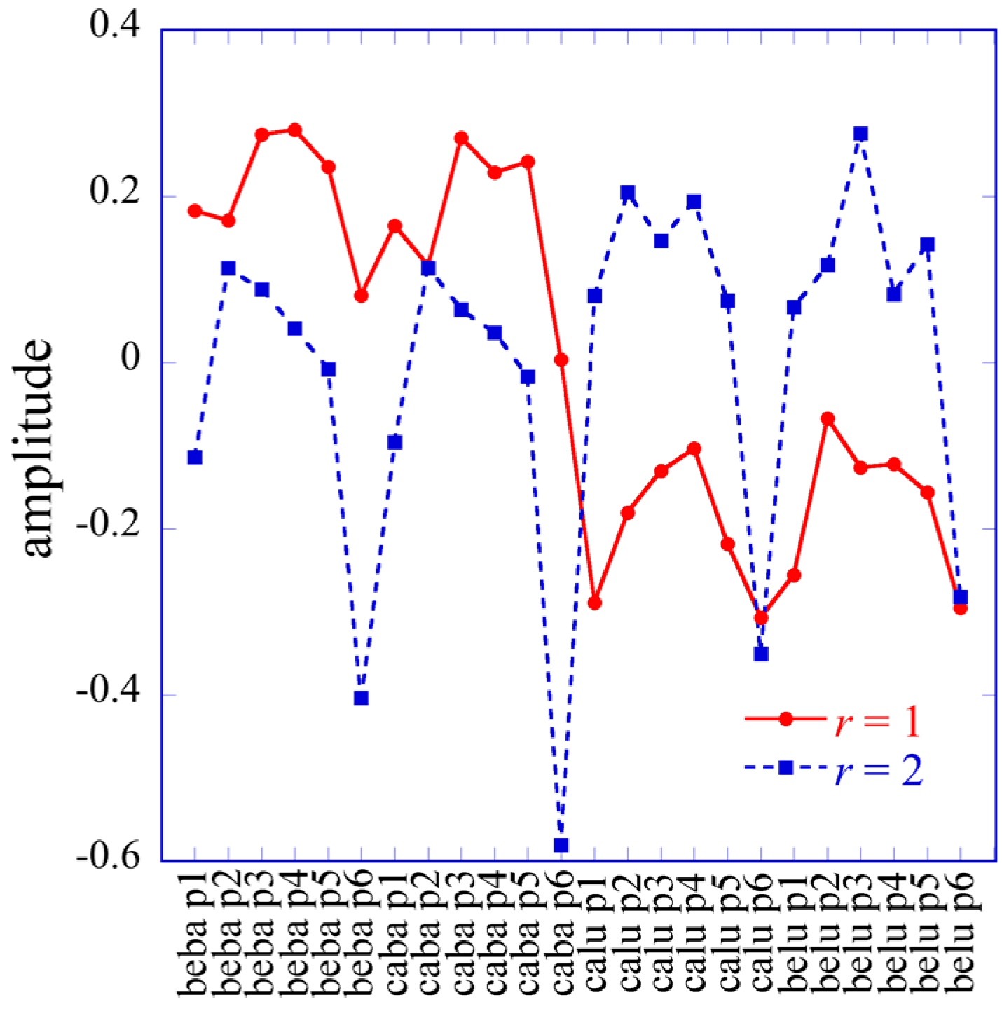The analysis of the gene transcripts that dominate the G_i0 constraint show that the pattern of the base line corresponds to the essential machinery of the cell [4]. For α > 0, the biological interpretation of the transcription patterns are defined by the analysis of the values of the Lagrange multipliers ${\lambda }_{\alpha j}$ on the different conditions j. Each constra G_iα corresponds to a pattern in the gene expression associated with the phenotype α. We will therefore use the terms transcription pattern and phenotype interchangeably where by phenotype we mean a biological process where all the participating genes act coherently (see Equation (1) or (7)). The analysis of the phenotypes α > 0 and of the gene expression patterns was shown to characterize the progression of cancer in cell lines [5,24].

3. Generalization of the Surprisal Analysis for a Multivariate Array

The need for a generalization of surprisal analysis arises from the availability of gene transcript levels measured, for example, for individual patients and for different conditions or for different cell types. Keeping the different patients as a separate dimension in addition to cell type leads to data in the format of a 3D array. Another case where one can have more than 2D arrays of data is that where different cell types are submitted to different conditions [31,32,33]. Of course, a 4D data or even higher is also possible.

To bring the 3D tensor into a surprisal form, we use HOSVD [26]. This approach ensures that the constraints remain linearly independent and reverts to the 2D case discussed above as a limit. As an illustration of the formalism we will use data arrays where the gene expression level of different cell types is measured for several individual patients. The 3D analysis allows us to propose an interpretation of the notion of disease and of patient diversity.

We consider a 3D array, T, for which the three dimensions are the number of gene transcripts, I, the number of cell types, J, and the number of patients, K. The elements of the tensor are defined as $T_{ijk}=\ln X_{ijk}$ where X_ijk is the measured expression level for transcript i of cell type j of patient k. The number of transcripts, of the order of 20,000, is typically much larger than the numbers of cell types or the number of patients. We have therefore a rectangular 3D I × J × K tensor where I >> J ≈ K. This inequality, typical of gene expression data where the number I of transcripts is very large, plus the fact that we typically want the expression levels to remain an axis, dictates the compaction of the 3D data to a 2D form as discussed next.

3.1. Representing the Tensor Surprisal T in Matrix Form

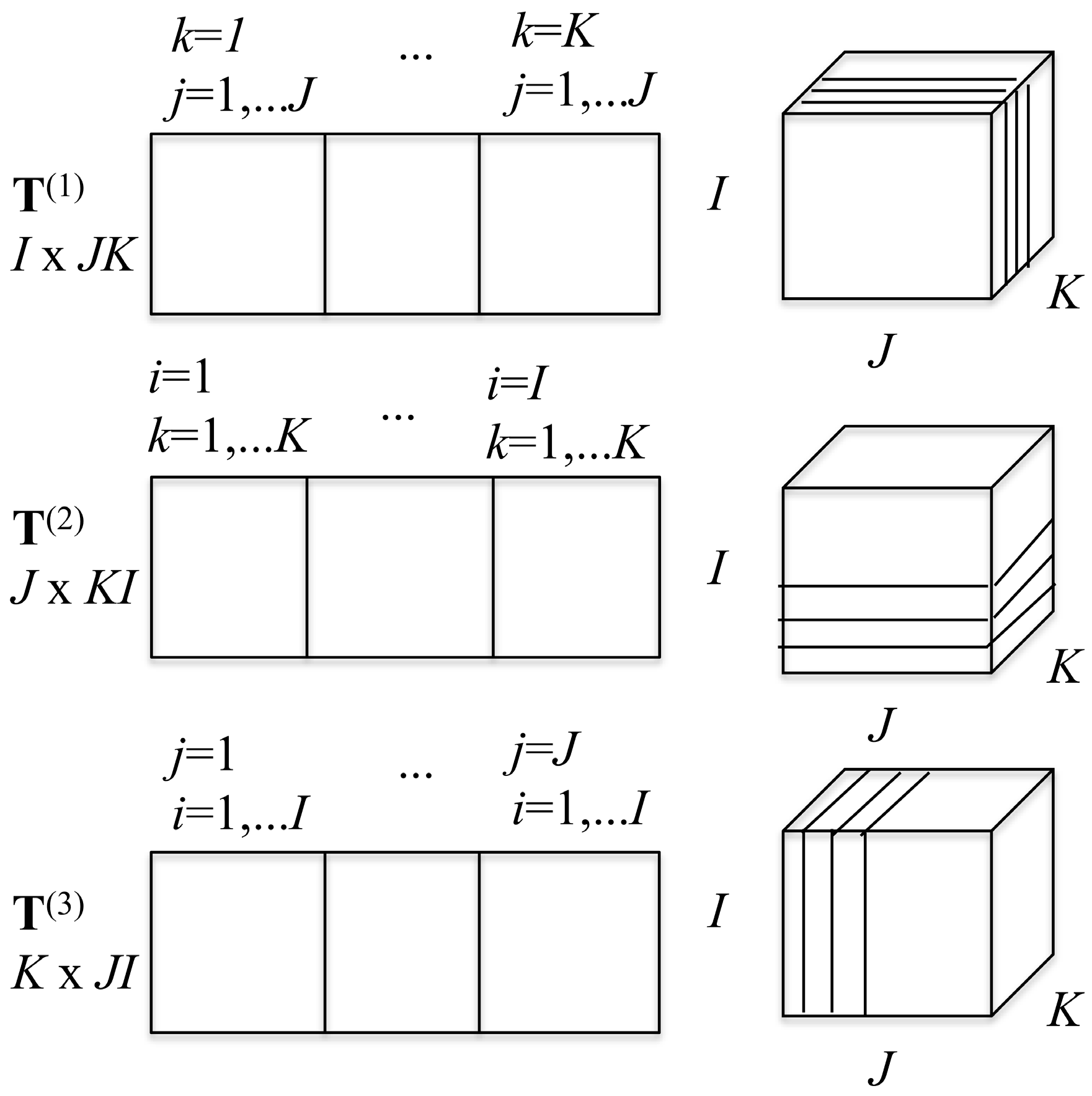
2D slices can be made from the 3D array in three ways. Keeping i fixed, one has I different J × K matrices, keeping j fixed, one has JK × I matrices, and keeping k fixed generates KI × J matrices. These three possible decompositions of the 3D tensor are arranged as shown in Scheme 1. From these three decompositions, one can build three matrices that possess the same information as the tensor itself, as is also shown in Scheme 1. The matrix T⁽¹⁾ is a 2D I × (J × K) matrix. T⁽¹⁾ is made of K side by side I × J slices. The matrix T⁽²⁾ is of dimension J × (K × I) and is made of I side by side (J × K) matrices and the matrix T⁽³⁾ of dimension K × (I × J) that is made of J side by side (K × I) matrices. The three matrices T⁽¹⁾, T⁽²⁾, and T⁽³⁾ are called the flattened matrices and correspond to the three ways to represent the tensor as a 2D matrix. These three flattened matrices are the basis for the high order SV decomposition of the tensor [26]. Each of these flattened rectangular matrices can be decomposed using the 2D SVD procedure as explained in Section 2 above. We get

$$T^{(1)}=U\cdot {\Omega }^{(1)}\cdot M^T$$

(11)

$$T^{(2)}=V\cdot {\Omega }^{(2)}\cdot N^T$$

(12)

$$T^{(3)}=W\cdot {\Omega }^{(3)}\cdot L^T$$

(13)

The SV decomposition of each of the three flattened matrices T⁽¹⁾, T⁽²⁾, and T⁽³⁾ is algebraically the same procedure as discussed in Section 2 above for the 2D surprisal matrix. In particular, since the rows of the three matrices are not mean centered, for each of them, the normalized eigenvector of the small covariance matrix that corresponds to the largest eigenvalue has uniform amplitudes given by $1/\sqrt{\dim }$ where dim is the smallest dimension of each matrix.

The left-hand side matrices in Equations (11)–(13) provide a SV decomposition for the elements of the 3D tensor [26]:

$$T_{ijk}={\displaystyle \sum _{r=0}^{JK-1}}{\displaystyle \sum _{s=0}^{J-1}}{\displaystyle \sum _{t=0}^{K-1}}{\mathrm{\Omega }}_{rst}{U}_{ir}{V}_{js}{W}_{kt}$$

(14)

where the matrix U is the I × JK matrix of the left eigenvectors of T⁽¹⁾, V the J × J matrix of the left eigenvectors of T⁽²⁾, and W the K × K matrix of the left eigenvectors of T⁽³⁾. Ω is the core tensor. Its dimensions are JK × J × K and correspond to the number of non-zero eigenvalues of the flattened matrices T⁽¹⁾, T⁽²⁾, and T⁽³⁾, respectively. The elements of the core tensor can be computed from its JK × JK flattened matrix Ω⁽¹⁾ [26] by

$$\begin{array}{l}{\mathbf{\Omega }}^{(1)}=U^T\cdot T^{(1)}\cdot \left(V\otimes W\right)\\ {\left({\mathbf{\Omega }}^{(1)}\right)}_{rq}={\displaystyle \sum _{i=0}^{I-1}}{U}_{ir}{\displaystyle \sum _{l=0}^{JK-1}}{\left(T^{(1)}\right)}_{il}{\left(V\otimes W\right)}_{lq}\end{array}$$

(15)

In Equation (15), the symbol ⊗ stands for the direct product of the V and W matrices (see Equations (12) and (13)), which leads to a square JK × JK Ω⁽¹⁾ matrix. The matrices U and T⁽¹⁾ are defined in Equation (11) above. Equation (15) is the practical form that can be used to compute the core tensor as a flattened matrix. Formally, the core tensor Ω is defined from the n mode multiplication [26,27] of the input tensor T by the three matrices U, V, and W:

$$\mathbf{\Omega }=T_{\times 1}{U}_{\times 2}{V}_{\times 3}W$$

(16)

where the symbol “×1” means to multiply the input tensor from the gene direction I by the I × KJ U matrix of the left eigenvectors of T⁽¹⁾ (Equation (11)), “×2” means to multiply T from the cell type direction J by the matrix V of the left eigenvectors of T⁽²⁾ (Equation (12)), and “×3”means to multiply T from the patient direction K by W (Equation (13)). By doing so, one obtains the core tensor Ω of dimensions JK × J × K whose flattened expression is given by Equation (15).

The labels of matrix elements as used in Equation (14) are, of course, arbitrary. However, once we made a particular choice it carried through. Specifically, because we use the index i to label transcripts, the notation $U_{ir}$ implies that r will index the transcription patterns where U is the left matrix of T⁽¹⁾ (Equation (11)). Similarly j is a cell type index so s will label cell type patterns where $V_{js}$ is an element of the left matrix of T⁽²⁾ (Equation (12)) while r is a patient type index.

3.2. The Tensor Form of the Surprisal

Equation (14) generates a fully separable expression for the tensor form of the surprisal for a 3D data array

$$T_{ijk}={\displaystyle \sum _{r=0}^{JK-1}}{\displaystyle \sum _{s=0}^{J-1}}{\displaystyle \sum _{t=0}^{K-1}}{\mathrm{\Omega }}_{rst}{U}_{ir}{V}_{js}{W}_{kt}$$

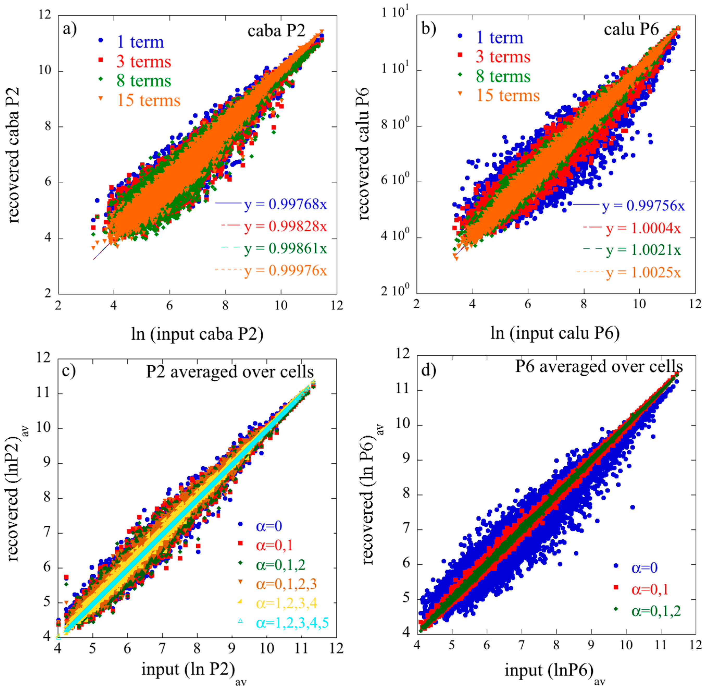
It takes JK × J × K terms to get an equality. The remarkable practical observation is that, in all the examples that we analyzed, very few terms need to be retained for this equation to provide an excellent approximation.

Equation (14) is analogous to Equation (3) of the 2D case. As in the 2D case it is possible to rewrite Equation (14) in a surprisal form. Here we discuss the surprisal of the expression level of the different transcripts, and since these are enumerated by the index i we pull the vector U up front in the summation. Rearrangement of the order of summations one has the 3D surprisal form as a summation over the different constraints labeled by r

$$\begin{array}{cc}\hfill T_{ijk}& {\displaystyle =\sum _{r=0}^{JK-1}}{\displaystyle \sum _{s=0}^{J-1}}{\displaystyle \sum _{t=0}^{K-1}}{\mathrm{\Omega }}_{rst}{U}_{ir}{V}_{js}{W}_{kt}\hfill \\ & ={\displaystyle \sum _{r=0}^{JK-1}}{U}_{ir}\left({\displaystyle \sum _{s=0}^{J-1}}{\displaystyle \sum _{t=0}^{K-1}}{\mathrm{\Omega }}_{rst}{V}_{js}{W}_{kt}\right)={\displaystyle \sum _{r=0}^{JK-1}}{U}_{ir}{\lambda }_{r\left(jk\right)}\hfill \end{array}$$

(17)

The Lagrange multiplier of the r’th constraint, ${\lambda }_{r\left(jk\right)}$, is thereby expressed as the term in the big bracket

$${\lambda }_{r\left(jk\right)}={\displaystyle \sum _{s=0}^{J-1}}{\displaystyle \sum _{t=0}^{K-1}}{\mathrm{\Omega }}_{rst}{V}_{js}{W}_{kt}$$

(18)

In the 2D case the Lagrange multipliers for a given constraint (a given value of α) form a vector. The entries of this vector are labeled by the different conditions j. In the 3D case the Lagrange multipliers are matrices, one matrix for each value of the index r of the constraints. (We use a different letter for the index of the constraints in 2 and 3D so as to explicitly indicate the dimension). The elements of each matrix are labeled by j and k, the indices of the different cell types and the different patients.

The entire set of Lagrange multipliers that were a matrix in the 2D case (Equation (9)) are now a 3D tensor Λ of dimension JK × J × K, $\mathbf{\Lambda }={\mathbf{\Omega }}_{\mathrm{x}2}{V^T}_{\mathrm{x}3}{W}^T$ whose flattened matrix form is given by

$${\mathbf{\Lambda }}^{(1)}={\mathbf{\Omega }}^{(1)}\cdot {\left(V\otimes W\right)}^T={\mathbf{\Omega }}^{(1)}\cdot \left(V^T\otimes W^T\right)$$

(19)

By analogy to the matrix product representation, Equation (10), of the 2D case, one can also rewrite the surprisal as given by Equation (17) as an n mode product of the tensor representing the Lagrange multipliers, Λ, by a matrix representing the constraints, U:

$$T={\mathbf{\Lambda }}_{\mathrm{x}1}U$$

(20)

3.3. The Lagrange Multipliers

Numbering the eigenvalues by decreasing order, we can rewrite the surprisal form (17) as

$$T_{ijk}=\frac{1}{\sqrt{KJ}}{U}_{i0}{\mathrm{\Omega }}_{000}+{\displaystyle \sum _{r=1}^{JK-1}}{U}_{ir}{\lambda }_{r(jk)}$$

(21)

where the first term is the base line for the 3D case, taking into account that

$$\begin{array}{l}{V}_{0j}=\frac{1}{\sqrt{J}},j=0,\dots ,J-1\\ W_{0k}=\frac{1}{\sqrt{K}},k=0,\dots ,K-1\end{array}$$

(22)

We stress that due to the condition on the dimensions of the tensor, I >> J ≈ K, the I components of the vector U₀ are not uniform. They define the gene transcript pattern that corresponds to the base line. The vector U₀ plays the role of the vector G₀ in the 2D case.

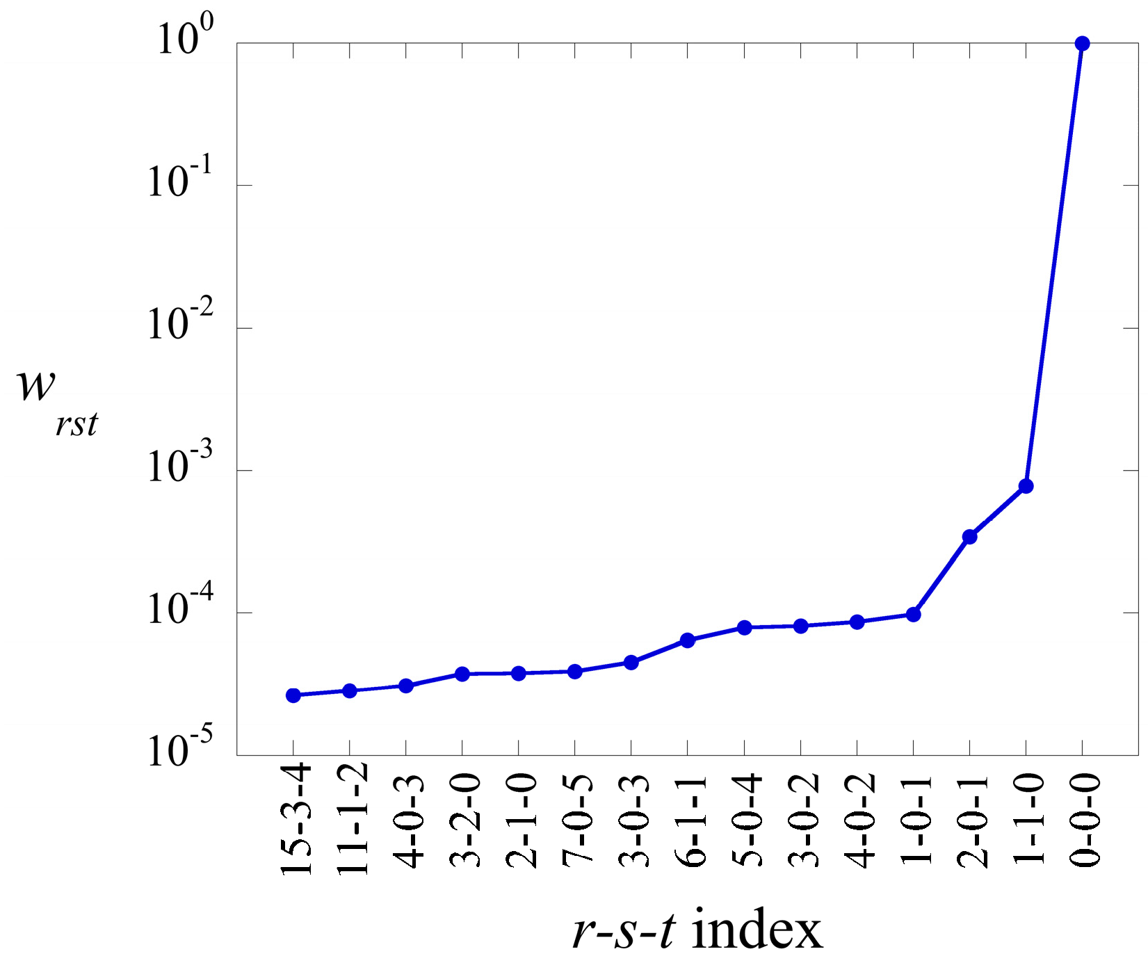
The elements of the core tensor, ${\mathrm{\Omega }}_{rst}$ in Equation (17), can be ranked in decreasing order. Their weight is defined as

$$w_{rst}=\frac{{\mathrm{\Omega }}_{rst}^2}{{\displaystyle \sum _{r=0}^{KJ-1}}{\displaystyle \sum _{s=0}^{J-1}}{\displaystyle \sum _{k=0}^{K-1}}{\omega }_{rst}^2}$$

(23)

The ${\mathrm{\Omega }}_{000}$ term has always the highest weight. This is the term that defines the baseline. As we show in the illustrative example below, this term alone usually provides a semiquantitatively acceptable fit of the data. Often, fewer than a dozen terms suffice to recover most of the information contained in the data.

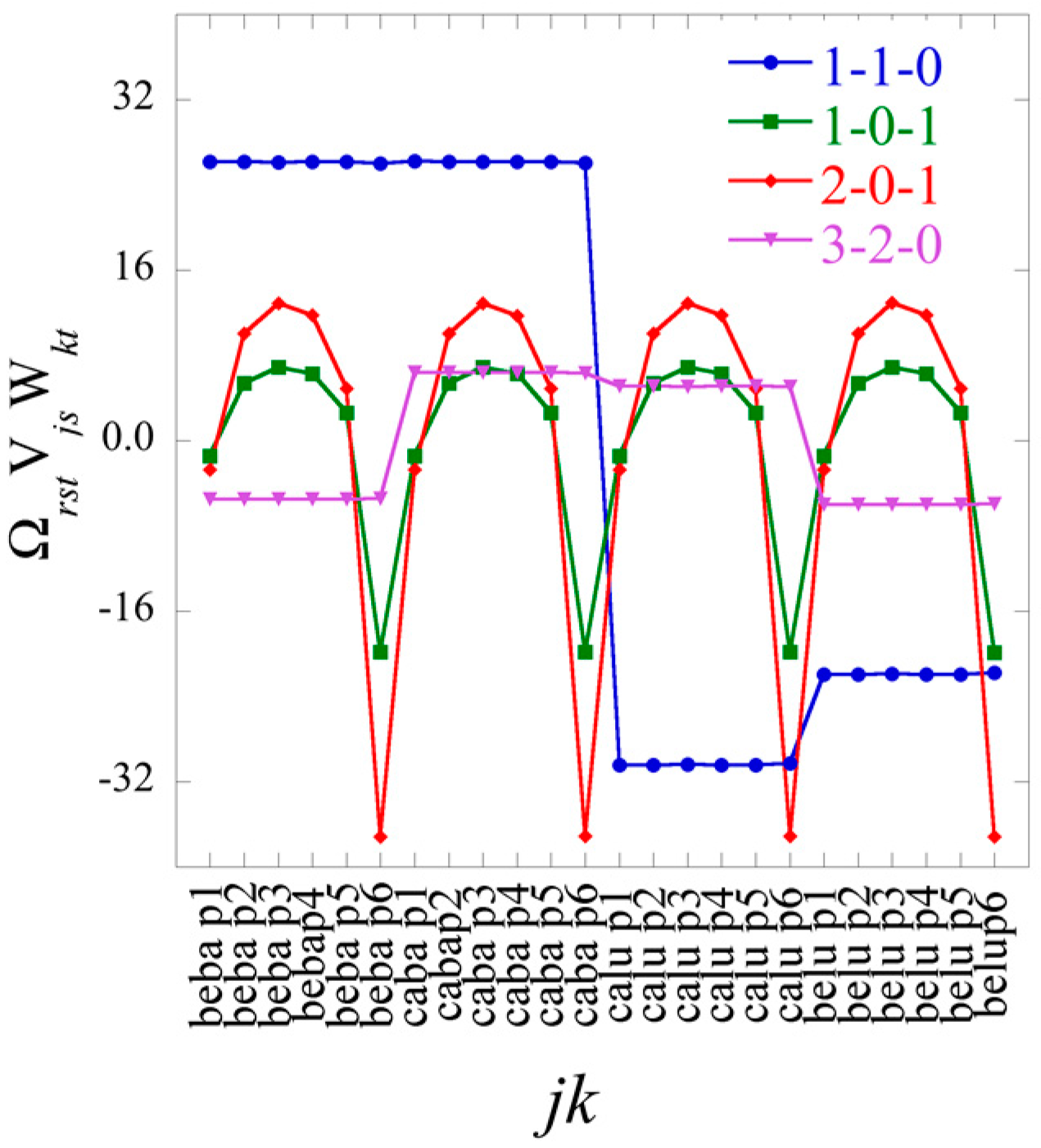
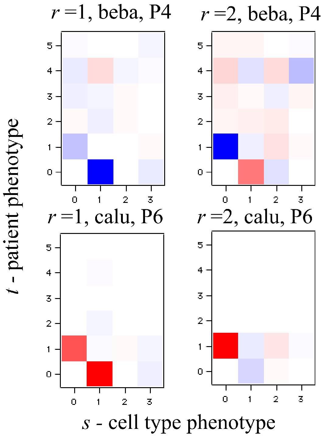
In Equation (21), each element of the tensor of the Lagrange multiplier ${\lambda }_{r\left(jk\right)}$

$${\lambda }_{r(jk)}={\displaystyle \sum _{s=0}^{J-1}}{\displaystyle \sum _{t=0}^{K-1}}{\mathrm{\Omega }}_{rst}{V}_{js}{W}_{kt}$$

(24)

can be represented as a J × K heat map. Among the J × K terms in the sum typically very few ones of the highest weight dominate. We show an example of such heat maps of the elements of the tensor of the Lagrange multipliers in the analysis of the numerical example below. Here we draw attention to a 2D view that also leads to this form for the surprisal. In this 2D view we arrange the 3D data as a 2D array by giving each data column a double index jk. On reflection this is exactly the matrix T⁽¹⁾ of dimension I × JK as discussed above. This matrix has JK non-zero eigenvalues. Its SV decomposition is given by Equation (11), where M is the matrix on the right:

$$T_{i(jk)}^{(1)}={\displaystyle \sum _{r=0}^{JK-1}{G}_{ir}}{\omega }_r{M}_{(jk)r}={\displaystyle \sum _{\alpha =0}^{JK-1}{G}_{ir}{\lambda }_{r(jk)}}$$

(25)

From the surprisal form (21), we have the equality

$${\lambda }_{r(jk)}={\omega }_r{M}_{(jk)r}={\displaystyle \sum _{s=0}^{J-1}}{\displaystyle \sum _{t=0}^{K-1}}{\mathrm{\Omega }}_{rst}{V}_{js}{W}_{kt}$$

(26)

3.4. 2D Limiting Forms of the Tensor Form of the Surprisal

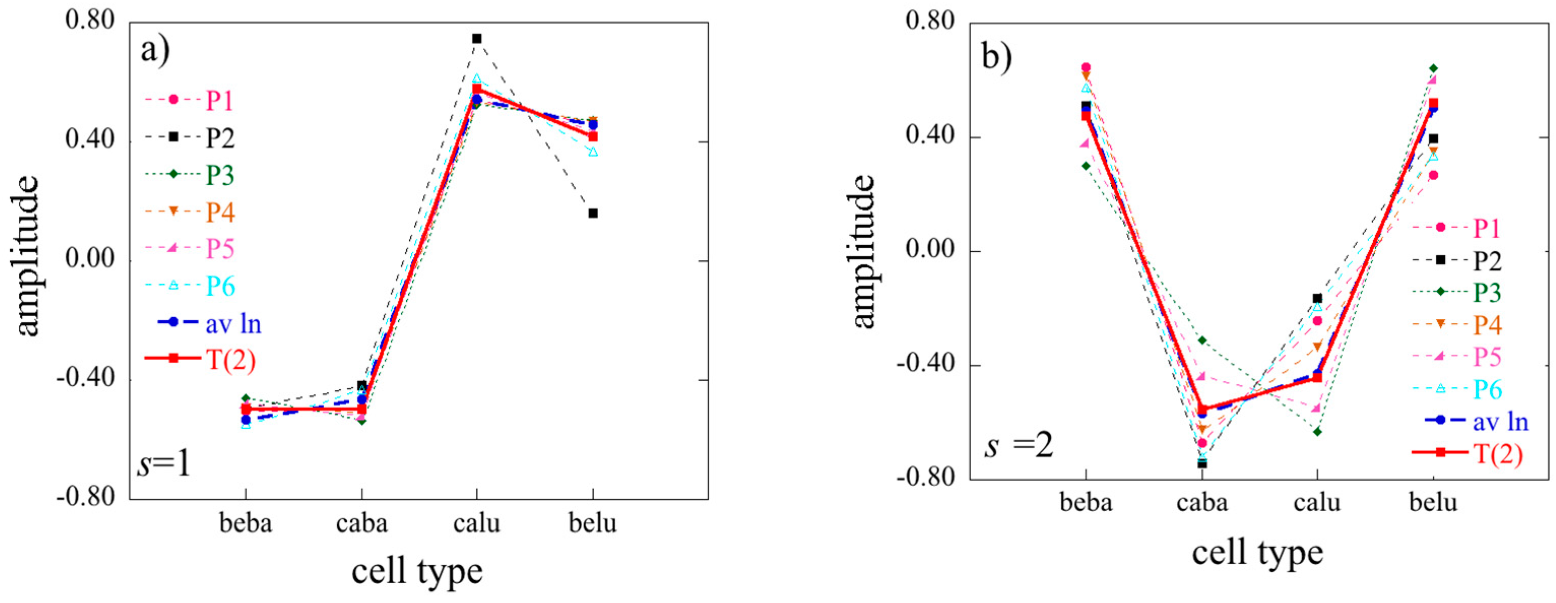
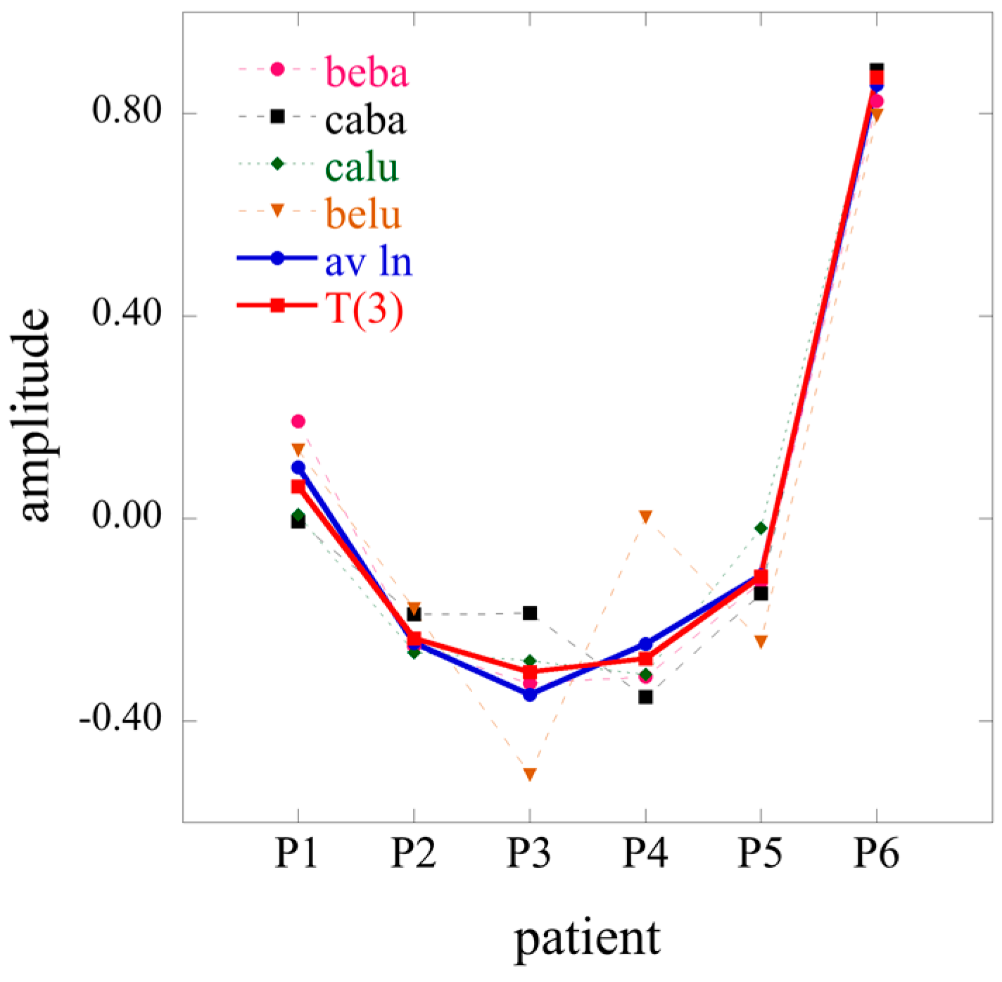
2D limits of the 3D surprisal enable us, for example, to analyze separately the correlations between cell types, irrespective of the patients or the correlations between patients irrespective of cell types. To do so one needs to average the data over patients or over cell type respectively. In the first case, one will get a 2D array of dimension I × J, and in the second one, a 2D array of dimension I × K. Using an overbar to designate an average we write when we average the surprisal

$$T_{ij\overline{k}}=\frac{1}{K}{\displaystyle \sum _{k=0}^{K-1}}{T}_{ijk}$$

(27)

$$T_{i\overline{j}k}=\frac{1}{J}{\displaystyle \sum _{j=0}^{J-1}}{T}_{ijk}$$

(28)

These two 2D matrices can be obtained by starting from the general surprisal form given by Equation (17) and, as we next show, retain only terms t = 0 (average over patients) or only terms s = 0 (average over cell type). From averaging over patients in the surprisal form of the tensor, Equation (27), takes the form:

$$\begin{array}{cc}\hfill T_{ij\overline{k}}& =\frac{1}{K}{\displaystyle \sum _{k=0}^{K-1}}{T}_{ijk}=\frac{1}{\sqrt{K}}{\displaystyle \sum _{r=0}^{KJ-1}}{U}_{ir}{\displaystyle \sum _{s=0}^{J-1}}{V}_{js}{\displaystyle \sum _{t=0}^{K-1}}{\mathrm{\Omega }}_{rst}{\displaystyle \sum _{k=0}^{K-1}}{W}_{kt}{W}_{k0}\hfill \\ & =\frac{1}{\sqrt{K}}{\displaystyle \sum _{r=0}^{KJ-1}}{U}_{ir}\left({\displaystyle \sum _{s=0}^{J-1}}{\mathrm{\Omega }}_{rs0}{V}_{js}\right)=\frac{1}{\sqrt{K}}{\displaystyle \sum _{r=0}^{KJ-1}}{U}_{ir}{\lambda }_{rj0}\hfill \end{array}$$

(29)

where Equation (22) and the orthogonality between the eigenvectors of T⁽³⁾ have been taken into account. Similarly, when averaging over cell types, one obtains

$$\begin{array}{cc}\hfill T_{i\overline{j}k}& =\frac{1}{J}{\displaystyle \sum _{j=0}^{J-1}}{T}_{ijk}=\frac{1}{\sqrt{J}}{\displaystyle \sum _{r=0}^{KJ-1}}{U}_{ir}{\displaystyle \sum _{t=0}^{K-1}}{W}_{kt}{\displaystyle \sum _{s=0}^{J-1}}{\mathrm{\Omega }}_{rst}{\displaystyle \sum _{j=0}^{J-1}}{V}_{js}{V}_{j0}\hfill \\ & =\frac{1}{\sqrt{J}}{\displaystyle \sum _{r=0}^{KJ-1}}{U}_{ir}\left({\displaystyle \sum _{t=0}^{K-1}}{W}_{kt}{\mathrm{\Omega }}_{r0t}\right)\hfill \\ & =\frac{1}{\sqrt{J}}{\displaystyle \sum _{r=0}^{KJ-1}}{U}_{ir}{\lambda }_{r0k}\hfill \end{array}$$

(30)

The expressions of Equations (29) and (30) are not fully identical to what one would get by applying 2D SVD directly to averaged I × J and I × K data matrices where the difference is that the logarithm of the average is not the same as the average of the logarithm (see also Section S1 of the supplementary materials).

By performing a double average over both patients and cell types, the 1D limit is given by

$$\begin{array}{cc}\hfill T_{i\overline{jk}}& =\frac{1}{JK}{\displaystyle \sum _{j=0}^{K-1}}{\displaystyle \sum _{k=0}^{K-1}}{T}_{ijk}\hfill \\ & =\frac{1}{\sqrt{JK}}{\displaystyle \sum _{r=0}^{KJ-1}}{U}_{ir}{\displaystyle \sum _{s=0}^{J-1}}{\displaystyle \sum _{t=0}^{K-1}}{\mathrm{\Omega }}_{rst}{\displaystyle \sum _{j=0}^{J-1}}{V}_{js}{V}_{j0}{\displaystyle \sum _{k=0}^{K-1}}{W}_{kt}{W}_{k0}\hfill \\ & =\frac{1}{\sqrt{JK}}{\displaystyle \sum _{r=0}^{KJ-1}}{U}_{ir}{\mathrm{\Omega }}_{r00}\hfill \end{array}$$

(31)

The 2D and even more so the 1D limit show how information is lost upon averaging. When 3D data is available the Lagrange multiplier for constraint r is given by, cf. Equation (17)

$${\lambda }_{r\left(jk\right)}=\left({\displaystyle \sum _{s=0}^{J-1}}{\displaystyle \sum _{t=0}^{K-1}}{\mathrm{\Omega }}_{rst}{V}_{js}{W}_{kt}\right)$$

(32)

When there is an averaging on either patient or cell type data

$${\lambda }_{r0k}={\displaystyle \sum _{t=0}^{K-1}}{\mathrm{\Omega }}_{r0t}{W}_{kt},{\lambda }_{rj0}={\displaystyle \sum _{s=0}^{J-1}}{\mathrm{\Omega }}_{rs0}{V}_{js}$$

while in the 1D case when averaging is over both

$${\lambda }_{r00}={\mathrm{\Omega }}_{r00}$$

(33)

4. Analysis of the Correlations between Cell Type and Patient in a Cohort of 6 Patients

Section 4 illustrates multivariate analysis of a data tensor where the gene level expressions are recorded for two cell types (basal or luminal) of six patients with a benign or advanced stage of prostate cancer. For each patient, there are therefore four cell types: benign luminal (BeLu), cancerous luminal (CaLu), benign basal (BeBa), and cancerous basal (CaBa). Each measurement was done in three replicates and only the genes that satisfied the confidence Student test were kept in the analysis. This leads to a data tensor of dimensions 18220 × 4 × 6.

4.1. Multivariate Surprisal Analysis

The starting point of the multivariate analysis of the surprisal is to compute the weights of the elements of the core tensor Ω_rst given by Equation (23). The highest ones are plotted in Figure 1. The base line element, Ω₀₀₀, dominates and with a weight (Equation (23)) equal to 0.99721 the base line accounts for 99.7% of the data. Also, in 2D expression level vs. time data the base line dominates [4] and it typically accounts for about 98% of the data. The next highest two elements are three orders of magnitude smaller and correspond to averaging over patient (1-1-0) and averaging over cell type (2-0-1). The three highest weight terms together represent 99.8% of the data. To interpret these results in terms of cell and patient phenotypes we plot the amplitudes Ω_rstV_jsW_kt of the terms 1-1-0 and 2-0-1 as a function of the combined cell type-patient index, Figure 2. Thereby it is seen that the 1-1-0 element of the tensor is a cell type phenotype and provides the distinction between basal and luminal cells, while the 2-0-1 is a patient phenotype which distinguishes between patient P6 and the rest of the patient. The amplitudes plotted in Figure 2 are the terms in the tensor expansion, Equation (14), and are the main contributors to tensor of the Lagrange multiplier ${\lambda }_{r\left(jk\right)}$ defined in Equation (24). To ascertain that these amplitudes dominate we show the heat map of the s and t terms that contribute to a given ${\lambda }_{r\left(jk\right)}$ shown in Figure 3. It is seen that indeed the largest terms are the 1-1-0 and 2-0-1 terms. The averaging over cell types term 1-0-1 is also shown in Figure 2. The pattern of its amplitude on the jk cell-type-patient index is very similar to that of the 2-0-1 term. Its weight amounts to 0.01% of the data. We also show in Figure 2 the amplitudes of a disease phenotype, the 3-2-0 term. This term has opposite amplitudes on the benign and cancer cells. As we further discuss in Section 4.2 below, a disease phenotype needs to have the value 2 for the index s. The 3-2-0 term is the highest weight term of this type that appears in the highest weight list. It is not dominant (see Figure 1). This term corresponds to the disease cell phenotype (s = 2) and an averaging over patients (t = 0).

In Figure 3 one can also see what are the other terms of the tensor form of the surprisal (Equation (17)), that mostly contribute to the value of the Lagrange multiplier ${\lambda }_{r\left(jk\right)}$ for a given cell type j and a given patient k. For example, it is clear from the heat map that more terms are needed to reproduce the cell type “benign basal” of patient P4 than the cell type “cancer luminal” of P6. This is in part due to the fact that the most important patient phenotype, t = 1, that emerges from our analysis is one that has an overwhelming weight in P6. The description of the individuality of P4 involves more patient phenotypes. This is the reason why most of the highest weight terms beyond the terms 1-1-0 and 2-0-1 involve a patient phenotype and averaging over cell type. The heat map of the terms that contribute to a given Lagrange multiplier ${\lambda }_{r\left(jk\right)}$ provides a quantitative analysis of the correlations between cell type and patient and opens the way to personalized medicine.

The detailed structure shown in Figure 3 can also be viewed as when the Lagrange multiplier ${\lambda }_{r\left(jk\right)}={\omega }_r{M}_{\left(jk\right)r}$ is plotted vs. the combined index jk. As discussed in connection with the derivation of Equation (26), this multiplier can also be viewed as a result of analysis of a 2D data matrix where each data column corresponds to a pair of conditions jk. Such a plot is shown for r = 1,2 in Figure 4. To plot two terms on a common scale we plot the amplitude $M_{\left(jk\right)r}$.

The base line and the two highest terms in the expansion of the tensor surprisal suffice to provide a very acceptable fit of the data (see Figure 5). The next five terms that are shown in Figure 1 serve mainly to distinguish among patients and correspond to an averaging over cell type. Terms that show correlations between cell type and patient, meaning both values of s and t are different from zero, have smaller weights.

Figure 5a shows the fit to the data for a given cell type and patient computed for an increasing number of terms in the expansion of the surprisal, Equation (17). The number of terms kept are one term, that corresponding to the 0-0-0 base line term, three terms (0-0-0, 1-1-0, and 2-0-1), eight terms, and 15 terms (see Figure 1 for the values of the indices). Keeping only three terms, terms that are just three entries of the core tensor, is already sufficient to provide a good fit for all the 24 combinations between cell type and patients. We also note that retaining three and eight terms does not significantly improve the fit obtained by retaining the base line only. Also shown in Figure 5b is the fit to the data, but from a 2D analysis where the patient data has been averaged over cell types. The point is to show how the tensor representation that keeps the cell-patient correlation explicitly has a richer and finer structure. Figure 5c,d show the 2D surprisal analysis of the input data. The 2D input matrix is obtained by averaging over cell type for each of the six patients. In such an analysis, the information over cell type is washed out. The Lagrange multiplier, ${\lambda }_{\alpha j}$, of a given constraint, α, is a vector that depends on the index j of the patient only (see Equation (1) and Section 2). For such averaging, the constraints correspond to a patient phenotype, irrespective of the cell type. One needs several patient phentoypes to satisfactorily recover the data for patient P2 (Figure 5c) while the data of patient P6 are well fitted with only two patient phenotypes.

4.2. Dominant Phenotypes Along Each Tensor Direction

We discuss the phenotypes as determined by the 3D tensor data and as approximated by the ensemble averaging approach discussed in detail in the supplementary materials file.

The “cell type” phenotypes are defined by the left eigenvectors of the matrix V of the flatten matrix T⁽²⁾, Equation (12). These eigenvectors are also those defining the phenotypes in the 2D limit given by Equations (27) and (28). Their importance is ranked by the magnitude of the eigenvalues. The eigenvalues of T⁽²⁾ are reported in Table S1 of the supplementary materials. As discussed, the largest eigenvalue corresponds to a uniform eigenvector whose amplitudes are given by $1/\sqrt{J}$ and this defines the base line. The amplitudes of the eigenvector corresponding to the next largest eigenvalue reflects the distinction between basal and luminal cells (see Figure 6a) while the next largest phenotype discriminates between benign and cancerous cells, Figure 6b. Beyond that, the phenotypes are becoming not so secure because they are increasingly more contaminated by noise. To assess the biology associated with disease, genes that discriminate between benign and cancerous cells were characterized into pathways using DAVID Bioinformatics [35]. Of note, the most significant pathways included immune response and several immune-related terms, supporting a role for the immune system in tumor development (Table S2).

To assess the robustness of these three phenotypes, we have also carried out the 2D SVD decomposition of the “gene transcript” vs “cell type” matrices for each of the six patients separately, as shown in Figure 6. The corresponding eigenvectors are reported in dotted lines in the figures and the eigenvalues in Table S1. As a last check, we analyzed the I × J matrix obtained by averaging the logarithm of the data over patients. For the off diagonal elements of the 2D covariance matrix there is a difference between averaging first and analyzing next or analyzing first and averaging the surprisal next.

For the dominant phenotype, that discriminates between basal and luminal cells, cf. Figure 6a, eigenvectors computed for each patient individually almost superimpose with those defined from the tensor analysis and by averaging over patients. For the next phenotypes that are related to the disease, there is somewhat more dispersion among the eigenvectors computed for individual patients, but the tensor analysis and the average over patient lead to very similar results. This indicates that the “cell phenotypes” are robust and common to all patients.

We turn next to the complementary aspect, that of the analysis of the “patient” phenotypes. Those are defined by the left eigenvectors, W, of the flattened T⁽³⁾ matrix (Equation (13)). Those eigenvectors also define the patient phenotype in the 2D analysis given by Equation (29). Similarly to the analysis of the “cell type” phenotypes, the “patient” phenotypes obtained from the tensor decomposition can be compared to those defined by the 2D SVD analysis of the average of logarithm of the data over cell types as well as those obtained for each cell type individually.

Unlike for the cell type analysis, the variations from patient to patient are more correlated to the cell type. Only two patient phenotypes, t = 1 (see Figure 7) and t = 2 are common to all cell types and even for those, there is more dispersion between the results for each cell type than between the results of each patient in the cell type analysis. The patient phenotype t = 1 indicates that patient 6 and to a certain extent patient 1 are different from the rest of the patients.

From t = 3 on, the patient-cell type correlations are too strong to be able to define a patient phenotype across all cell types. In that case, the tensor phenotype is different from that obtained by averaging over cell type.

5. Conclusions

The multivariate surprisal analysis of the gene transcript expression levels measured for several cell types of different patients allows us to characterize the gene expression of dominant cell type and patient phenotypes. In the case of the data that we have analyzed, the dominant cell phenotype distinguishes between basal and luminal cells, irrespective of the benign or cancer disease character. The next cell phenotype is the disease phenotype, that discriminates between benign and cancer, irrespective of the cell type. The patient analysis shows that patient P6 is different from the rest of the five patients. A second patient phenotype indicates that P1 and P6 are different from P2, P3, P4, and P5.

The tensor analysis shows that beyond the distinction between basal and luminal cells, the data are dominated by the patient to patient variations. The tensor analysis thereby opens the way to a quantification of the correlations between cell types and patients and could therefore contribute towards personalized diagnostics and intervention.

References

1. Alhassid, Y.; Levine, R.D. Connection between maximal entropy and scattering theoretic analyses of collision processes. Phys. Rev. A 1978, 18, 89–116. [Google Scholar] [CrossRef]
2. Levine, R.D. Information theory approach to molecular reaction dynamics. Annu. Rev. Phys. Chem. 1978, 29, 59–92. [Google Scholar] [CrossRef]
3. Levine, R.D.; Bernstein, R.B. Energy disposal and energy consumption in elementary chemical reactions. Information theoretic approach. Acc. Chem. Res. 1974, 7, 393–400. [Google Scholar] [CrossRef]
4. Kravchenko-Balasha, N.; Levitzki, A.; Goldstein, A.; Rotter, V.; Gross, A.; Remacle, F.; Levine, R.D. On a fundamental structure of gene networks in living cells. Proc. Natl. Acad. Sci. USA 2012, 109, 4702–4707. [Google Scholar] [CrossRef] [PubMed]
5. Remacle, F.; Kravchenko-Balasha, N.; Levitzki, A.; Levine, R.D. Information-theoretic analysis of phenotype changes in early stages of carcinogenesis. Proc. Natl. Acad. Sci. USA 2010, 107, 10324–10329. [Google Scholar] [CrossRef] [PubMed]
6. Zadran, S.; Remacle, F.; Levine, R.D. miRNA and mRNA cancer signatures determined by analysis of expression levels in large cohorts of patients. Proc. Natl. Acad. Sci. USA 2013, 110, 19160–19165. [Google Scholar] [CrossRef] [PubMed]
7. Remacle, F.; Levine, R.D. Statistical thermodynamics of transcription profiles in normal development and tumorigeneses in cohorts of patients. Eur. Biophys. J. 2015, 44, 709–726. [Google Scholar] [CrossRef] [PubMed]
8. Zadran, S.; Arumugam, R.; Herschman, H.; Phelps, M.E.; Levine, R.D. Surprisal analysis characterizes the free energy time course of cancer cells undergoing epithelial-to-mesenchymal transition. Proc. Natl. Acad. Sci. USA 2014, 109, 4702–4707. [Google Scholar] [CrossRef] [PubMed]
9. Mora, T.; Walczak, A.; Bialek, W.; Callan, C.G., Jr. Maximum entropy models for antibody diversity. Proc. Natl. Acad. Sci. USA 2009, 107, 5405–5410. [Google Scholar] [CrossRef] [PubMed]
10. Lezon, T.R.; Banavar, J.R.; Cieplak, M.; Maritan, A.; Fedoroff, N.V. Using the principle of entropy maximization to infer genetic interaction networks from gene expression patterns. Proc. Natl. Acad. Sci. USA 2006, 103, 19033–19038. [Google Scholar] [CrossRef] [PubMed]
11. Aghagolzadeh, M.; Soltanian-Zadeh, H.; Araabi, B.N. Information theoretic hierarchical clustering. Entropy 2011, 13, 450–465. [Google Scholar] [CrossRef]
12. Margolin, A.A.; Nemenman, I.; Basso, K.; Wiggins, C.; Stolovitzky, G.; Dalla Favera, R.; Califano, A. Aracne: An algorithm for the reconstruction of gene regulatory networks in a mammalian cellular context. BMC Bioinform. 2006, 7 (Suppl. S1), S7. [Google Scholar] [CrossRef] [PubMed]
13. Margolin, A.A.; Califano, A. Theory and limitations of genetic network inference from microarray data. Ann. N. Y. Acad. Sci. 2007, 1115, 51–72. [Google Scholar] [CrossRef] [PubMed]
14. Yeung, M.K.; Tegner, J.; Collins, J.J. Reverse engineering gene networks using singular value decomposition and robust regression. Proc. Natl. Acad. Sci. USA 2002, 99, 6163–6168. [Google Scholar] [CrossRef] [PubMed]
15. Shin, Y.S.; Remacle, F.; Fan, R.; Hwang, K.; Wei, W.; Ahmad, H.; Levine, R.D.; Heath, J.R. Protein signaling networks from single cell fluctuations and information theory profiling. Biophys. J. 2011, 100, 2378–2386. [Google Scholar] [CrossRef] [PubMed]
16. Schneidman, E.; Still, S.; Berry, M.J.; Bialek, W. Network information and connected correlations. Phys. Rev. Lett. 2003, 91, 238701. [Google Scholar] [CrossRef] [PubMed]
17. Rosvall, M.; Bergstrom, C.T. An information-theoretic framework for resolving community structure in complex networks. Proc. Natl. Acad. Sci. USA 2007, 104, 7327–7331. [Google Scholar] [CrossRef] [PubMed]
18. Quigley, D.A.; To, M.D.; Kim, I.J.; Lin, K.K.; Albertson, D.G.; Sjolund, J.; Pérez-Losada, J.; Balmain, A. Network analysis of skin tumor progression identifies a rewired genetic architecture affecting inflammation and tumor susceptibility. Genome Biol. 2011, 12, R5. [Google Scholar] [CrossRef] [PubMed] [Green Version]
19. Nykter, M.; Price, N.D.; Larjo, A.; Aho, T.; Kauffman, S.A.; Yli-Harja, O.; Shmulevich, I. Critical networks exhibit maximal information diversity in structure-dynamics relationships. Phys. Rev. Lett. 2008, 100, 058702. [Google Scholar] [CrossRef] [PubMed]
20. Alter, O. Genomic signal processing: From matrix algebra to genetic networks. In Microarray Data Analysis: Methods and Applications; Korenberg, M.J., Ed.; Humana Press: Totowa, NJ, USA, 2007. [Google Scholar]
21. Golub, T.R.; Slonim, D.K.; Tamayo, P.; Huard, C.; Gaasenbeek, M.; Mesirov, J.P.; Coller, H.; Loh, M.L.; Downing, J.R.; Caligiuri, M.A.; et al. Molecular classification of cancer: Class discovery and class prediction by gene expression monitoring. Science 1999, 286, 531–537. [Google Scholar] [CrossRef] [PubMed]
22. Gross, A.; Levine, R.D. Surprisal analysis of transcripts expression levels in the presence of noise: A reliable determination of the onset of a tumor phenotype. PLoS ONE 2013, 8, e61554. [Google Scholar] [CrossRef] [PubMed]
23. Gross, A.; Li, C.M.; Remacle, F.; Levine, R.D. Free energy rhythms in saccharomyces cerevisiae: A dynamic perspective with implications for ribosomal biogenesis. Biochemistry 2013, 52, 1641–1648. [Google Scholar] [CrossRef] [PubMed]
24. Kravchenko-Balashaa, N.; Remacle, F.; Gross, A.; Rotter, V.; Levitzki, A.; Levine, R.D. Convergence of logic of cellular regulation in different premalignant cells by an information theoretic approach. BMC Syst. Biol. 2011, 5, 42. [Google Scholar] [CrossRef] [PubMed]
25. Wei, W.; Shi, Q.H.; Remacle, F.; Qin, L.D.; Shackelford, D.B.; Shin, Y.S.; Mischel, P.S.; Levine, R.D.; Heath, J.R. Hypoxia induces a phase transition within a kinase signaling network in cancer cells. Proc. Natl. Acad. Sci. USA 2013, 110, E1352–E1360. [Google Scholar] [CrossRef] [PubMed]
26. De Lathauwer, L.; De Moor, B.; Vandewalle, J. A multilinear singular value decomposition. SIAM J. Matrix Anal. Appl. 2000, 21, 1253–1278. [Google Scholar] [CrossRef]
27. Kolda, T.G.; Bader, B.W. Tensor decompositions and applications. SIAM Rev. 2009, 51, 455–500. [Google Scholar] [CrossRef]
28. Tucker, L.R. Some mathematical notes on three-mode factor analysis. Psychometrika 1966, 31, 279–311. [Google Scholar] [CrossRef] [PubMed]
29. Alon, U. An Introduction to Systems Biology; CRC Press: Boca Raton, FL, USA, 2007. [Google Scholar]
30. Willamme, R.; Alsafra, Z.; Arumugam, R.; Eppe, G.; Remacle, F.; Levine, R.D.; Remacle, C. Metabolomic analysis of the green microalga chlamydomonas reinhardtii cultivated under day/night conditions. J. Biotechnol. 2015, 215, 20–26. [Google Scholar] [CrossRef] [PubMed]
31. Omberg, L.; Golub, G.H.; Alter, O. A tensor higher-order singular value decomposition for integrative analysis of DNA microarray data from different studies. Proc. Natl. Acad. Sci. USA 2007, 104, 18371–18376. [Google Scholar] [CrossRef] [PubMed]
32. Ponnapalli, S.P.; Saunders, M.A.; Van Loan, C.F.; Alter, O. A higher-order generalized singular value decomposition for comparison of global mrna expression from multiple organisms. PLoS ONE 2011, 6, e28072. [Google Scholar] [CrossRef] [PubMed]
33. Sankaranarayanan, P.; Schomay, T.E.; Aiello, K.A.; Alter, O. Tensor GSVD of patient- and platform-matched tumor and normal DNA copy-number profiles uncovers chromosome arm-wide patterns of tumor-exclusive platform-consistent alterations encoding for cell transformation and predicting ovarian cancer survival. PLoS ONE 2015, 10, e0121396. [Google Scholar] [CrossRef] [PubMed]
34. Zadran, S.; Remacle, F.; Levine, R.D. Microfluidic chip with molecular beacons detects miRNAs in human CSF to reliably characterize CNS-specific disorders. RNA Dis. 2016, 3, e1183. [Google Scholar]
35. Huang, D.W.; Sherman, B.T.; Lempicki, R.A. Systematic and integrative analysis of large gene lists using david bioinformatics resources. Nat. Protoc. 2008, 4, 44–57. [Google Scholar] [CrossRef] [PubMed]
Scheme 1. The three ways of representing the tensor T as two dimensional, Equations (11)–(13).
Entropy 18 00445 sch001
Figure 1. The 15 highest weights w r s t (Equation (23)) of the core tensor plotted on a logarithmic scale in decreasing order. Note the sheer drop beyond 0-0-0. Including terms on or beyond 4-0-3 only serves to fit the experimental noise in the data. See also Figure 4.
Entropy 18 00445 g001
Figure 2. The magnitude of the two highest weight terms (r-s-t = 1-1-0, 2-0-1) of the tensor form of the surprisal as a function of the jk index, conditionpatient. The first two highest terms, 1-1-0 and 2-0-1, already provide a very good fit for the surprisal. The phenotypes r = 1 and r = 2 are shown in Figure 3 and Figure 4 below. While r = 1 mainly corresponds to the distinction between basal and luminal cells with a small modulation due to the patients, r = 2 corresponds to the distinction between P6 and P1 and the rest of the patients with a small modulation due to the cell type. In this sense, 2-0-1 is more clearly a patient phenotype than 1-0-1. The term 3-2-0 is the first disease term. As shown, it distinguishes between benign and cancer cells in that it changes its sign. It is the 12th term in the tensor expansion (see Figure 1 for the weights, w r s t ) of the different terms and so it does not contribute much to the recovery of the input data.
Entropy 18 00445 g002
Figure 3. The magnitudes of the 24 terms ΩrstVjsWkt (see Equations (17) and (18)) that contribute to the value of a Lagrange multiplier λ r ( j k ) plotted as a heat map as a function of the cell phenotype index s and the patient phenotype t, r is the index of the constraint. Analyzing the relative importance of the different terms for a given constraint r and a given cell type and patient gives access to personalized medicine. Top left: r = 1, j = beba, k = P4, top right r = 2, j = beba, k = P4, bottom left: r =1, j = calu, k = P6, bottom right: r = 2, j = beba, k = P4. Note that the terms s = 1, t = 0, and s = 0 and t = 1 dominates all panels. In addition, the heat maps clearly indicate that more terms significantly contribute to a given cell type for patient P4 than P6. This can be understood because several patient phenotypes contribute to the description of P4.
Entropy 18 00445 g003
Figure 4. Amplitudes M ( j k ) r of the two dominant patterns, r = 1,2, of the bivariate transcription data matrix with 24 columns labeled by both cell type and patient. The r = 1 pattern is high on basal cells and low on luminal for each patient. The r = 2 pattern distinguishes patient 6 from the rest.
Entropy 18 00445 g004
Figure 5. Scatter plots of the recovered data vs. the input data for given cell type and patient and for a 2D computation that is done for data averaged over cell types. Shown in panels (a) and (b) are the cell type caba for P2 and calu for P6, respectively. The recovered data are computed for an increasing number of terms in the surprisal expansion. In the tensor analysis, panels (a) and (b), one (only the base line), three, eight, and fifteen terms are kept. There are 24 combinations of patients and cell types and there are thousands of transcription levels for each pair. For all 24 pairs the three terms suffice to characterize the data. Eight terms are needed for representation of details and from twelve terms on the fit is to the noise in the data. The RNA profile calu of P6 which is characterized by the first patient phenotype in the tensor analysis is better fitted than the caba profile of P2 that is spread over several patient phenotypes. In panels (c) and (d) where the data is averaged over cell types, two terms beyond the base line α = 0 capture most of P6 (d), which is characterized by the first phenotype patient. Many more terms are need for P2, because the RNA profile is described by several patient phenotypes.
Entropy 18 00445 g005
Figure 6. Amplitudes of the dominant cell type eigenvector Vjs, (a) for s = 1 and (b) for s = 2 on the four cell types, j = 1,2,3,4. Bold full line (red, color on line), computed for the diagonalization of the T(2) matrix, cf. Equation (12). Bold dashes (blue, color on line), computed from the diagonalization of the 2D matrix obtained by averaging the logarithm of the data over patients (see Section S1 of the supplementary materials). Thin lines, computed by 2D SVD analysis of the surprisal for each one of the six patients. For the dominant phenotype, which corresponds to the distinction between basal and luminal cells, all methods of analysis concur. s = 2 is the “disease” phenotype and distinguishes between benign and cancer cells. While there is a wider dispersion from one patient to the next, the tensor analysis and the average over patients give similar results.
Entropy 18 00445 g006
Figure 7. Amplitudes Wkt of the patient eigenvector, t = 1, on the six patients, k = 1,2,..,6. Bold full line (red, color on line), computed for the diagonalization of the T(3) matrix (Equation (13)). Bold dashes (blue, color on line), computed from the diagonalization of the 2D matrix obtained by averaging first over patients and then performing surprisal analysis. Thin lines, computed for each of the four cell types individually. The patient-cell type correlations are manifested strongly in the patient phenotype analysis which leads to a larger dispersion among the patient analysis for given cell types. Note, however, that the tensor analysis and the averaging over patients give similar results.
Entropy 18 00445 g007