
Bayesian Dependence Tests for Continuous, Binary and Mixed Continuous-Binary Variables

Abstract
:1. Introduction
2. Dirichlet Process
- (a)
- In case , since P is completely defined by its cumulative distribution function F, a-priori we say and a posteriori we can rewrite (3) as follows:where I is the indicator function and is the empirical cumulative distribution.
- (b)
- Consider an element which puts all its mass at the probability measure for some . This can also be modeled as for each .
- (c)
- Assume that , , and , , are independent, then Section 3.1.1. in [17]:
- (d)
- Let have distribution . We can writewhere , and . This follows from (b)–(c).
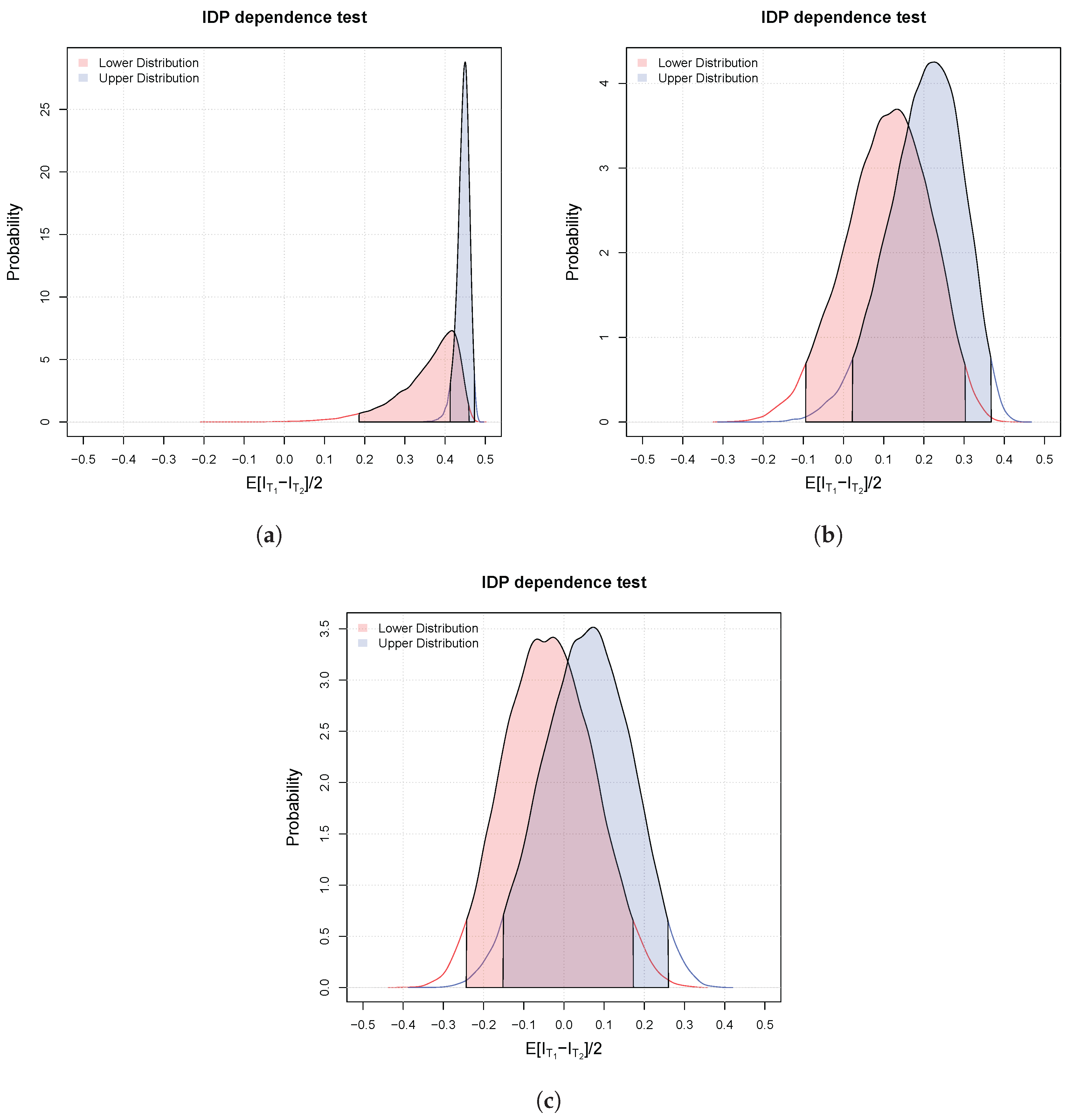
3. Bayesian Independence Tests
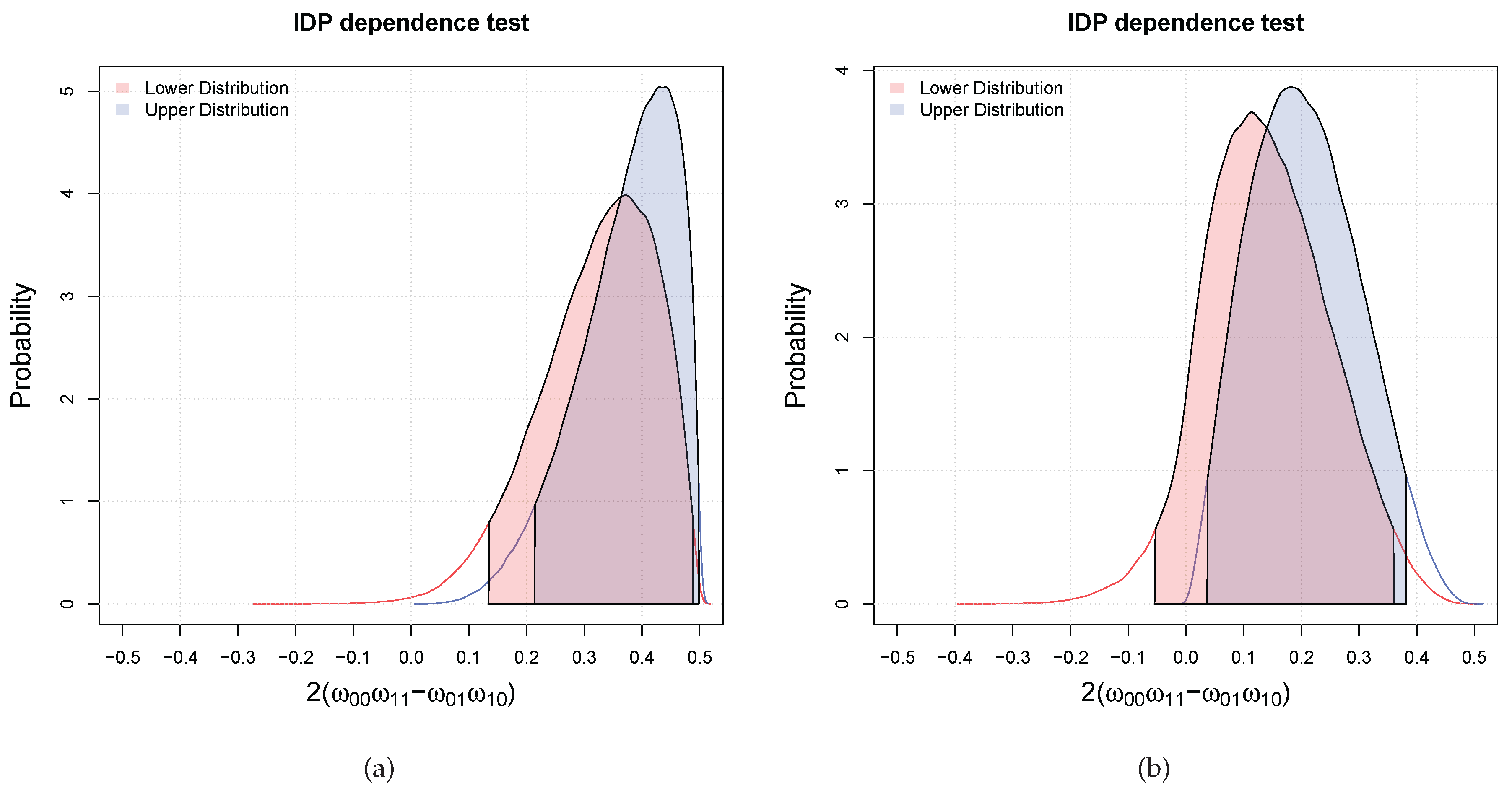
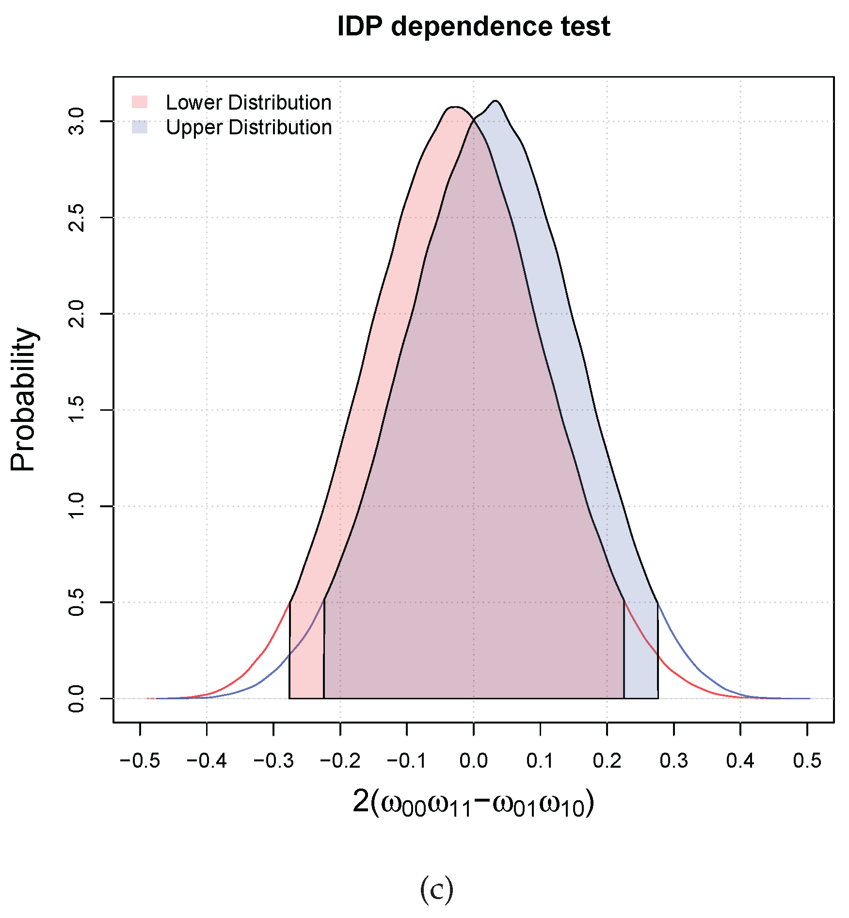
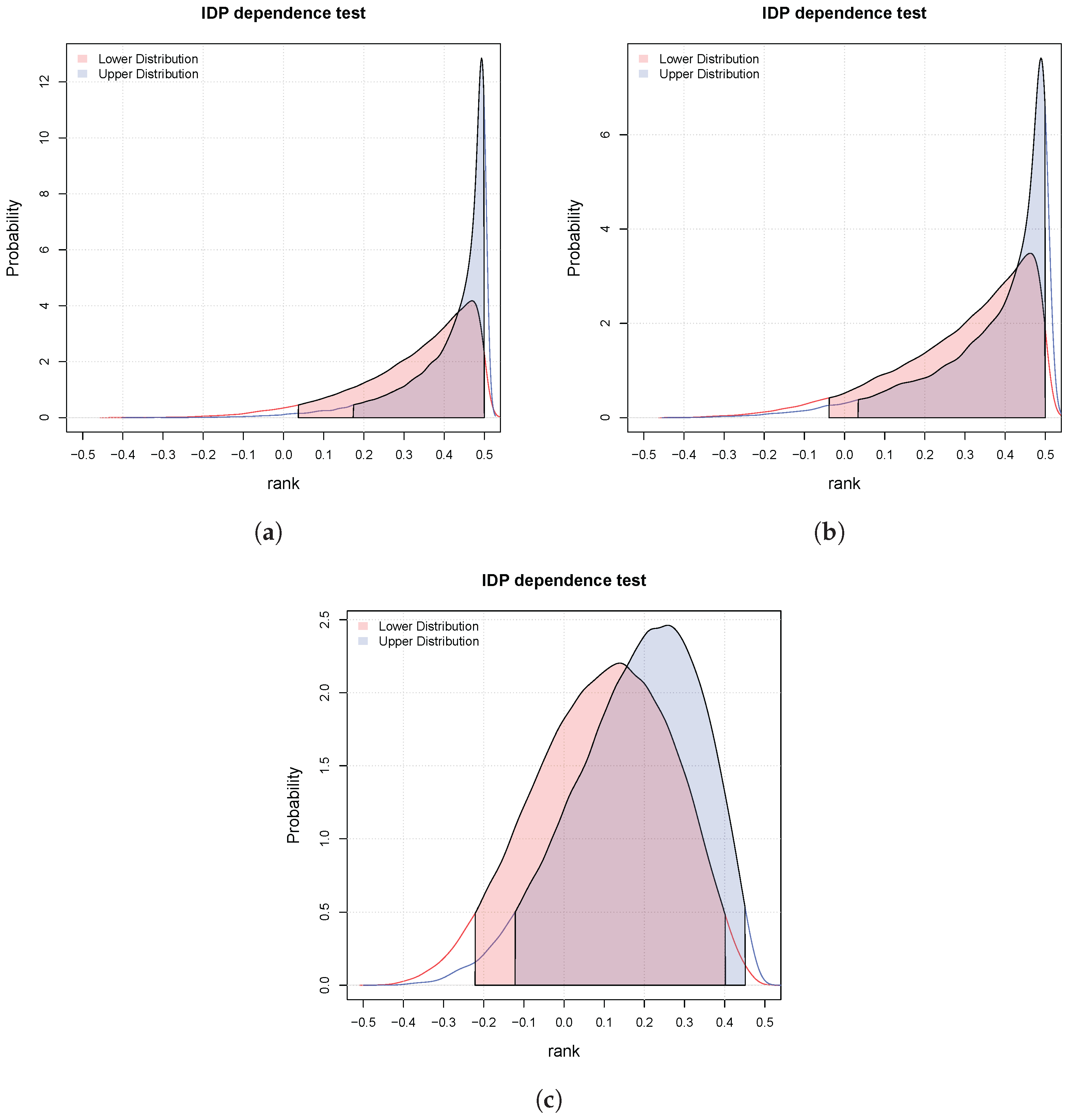
3.1. Bayesian Bivariate Independence Test for Binary Variables
- if both the inequalities are satisfied, then we declare that the two variables are dependent with probability larger than ;
- if only one of the inequalities is satisfied (which has necessarily to be the one for the upper), we are in an indeterminate situation, that is, we cannot decide;
- if both are not satisfied, then we declare that the probability that the two variables are dependent is lower than the desired probability of .
- Initialize the counter to 0 and the array V to empty;
- For
- (a)
- sample ;
- (b)
- compute as in (9)–(12) by choosing with m defined in Theorem 2;
- (c)
- compute and store the result in V;
- (d)
- if then else .
- compute the histogram of the elements in V (this gives us the plot of the posterior of )
- compute the posterior upper probability that is greater than zero as .
3.2. Bayesian Bivariate Independence Test for Continuous Variables
3.3. Bayesian Bivariate Independence Test for Mixed Continuous-Binary Variables
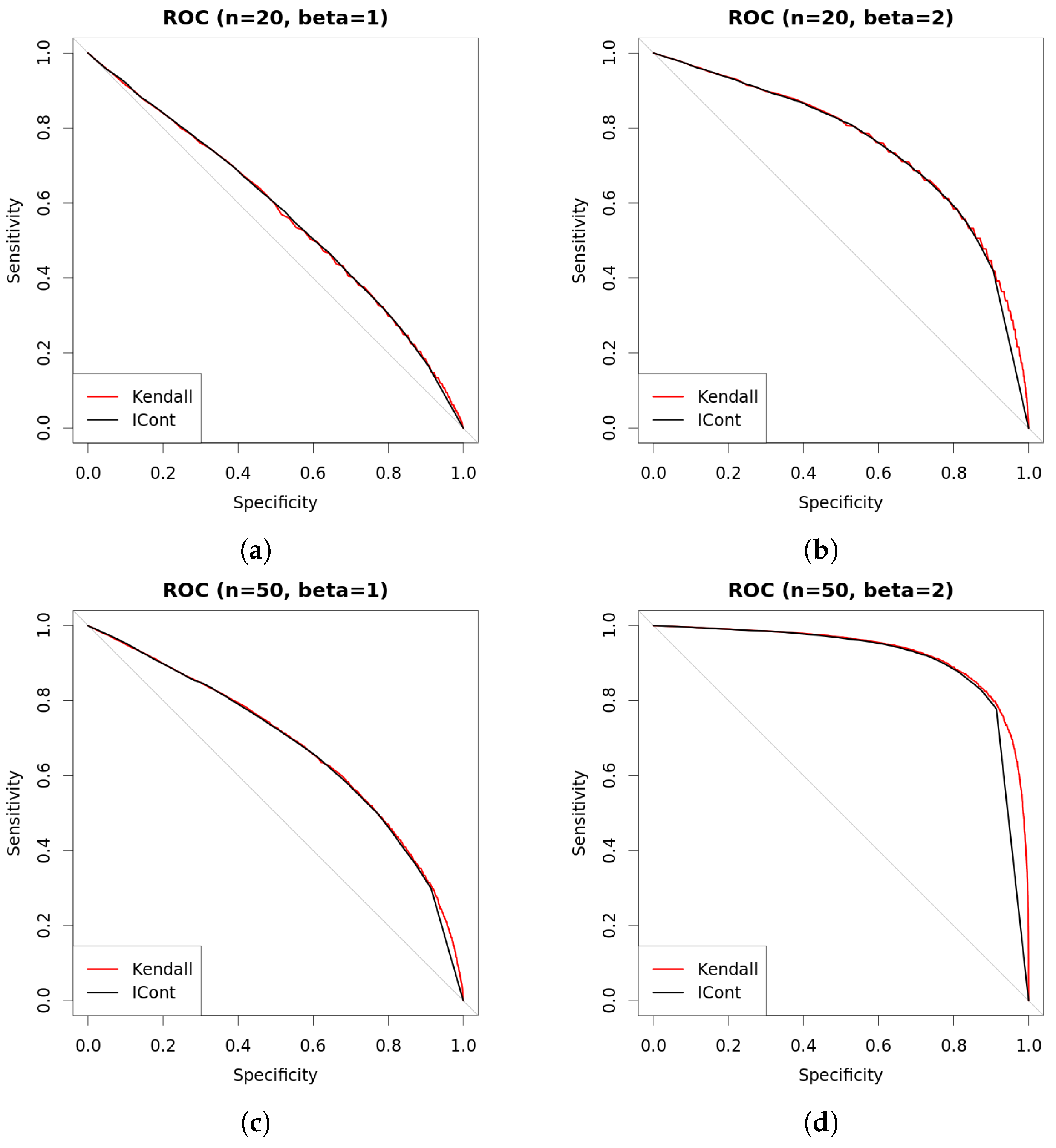
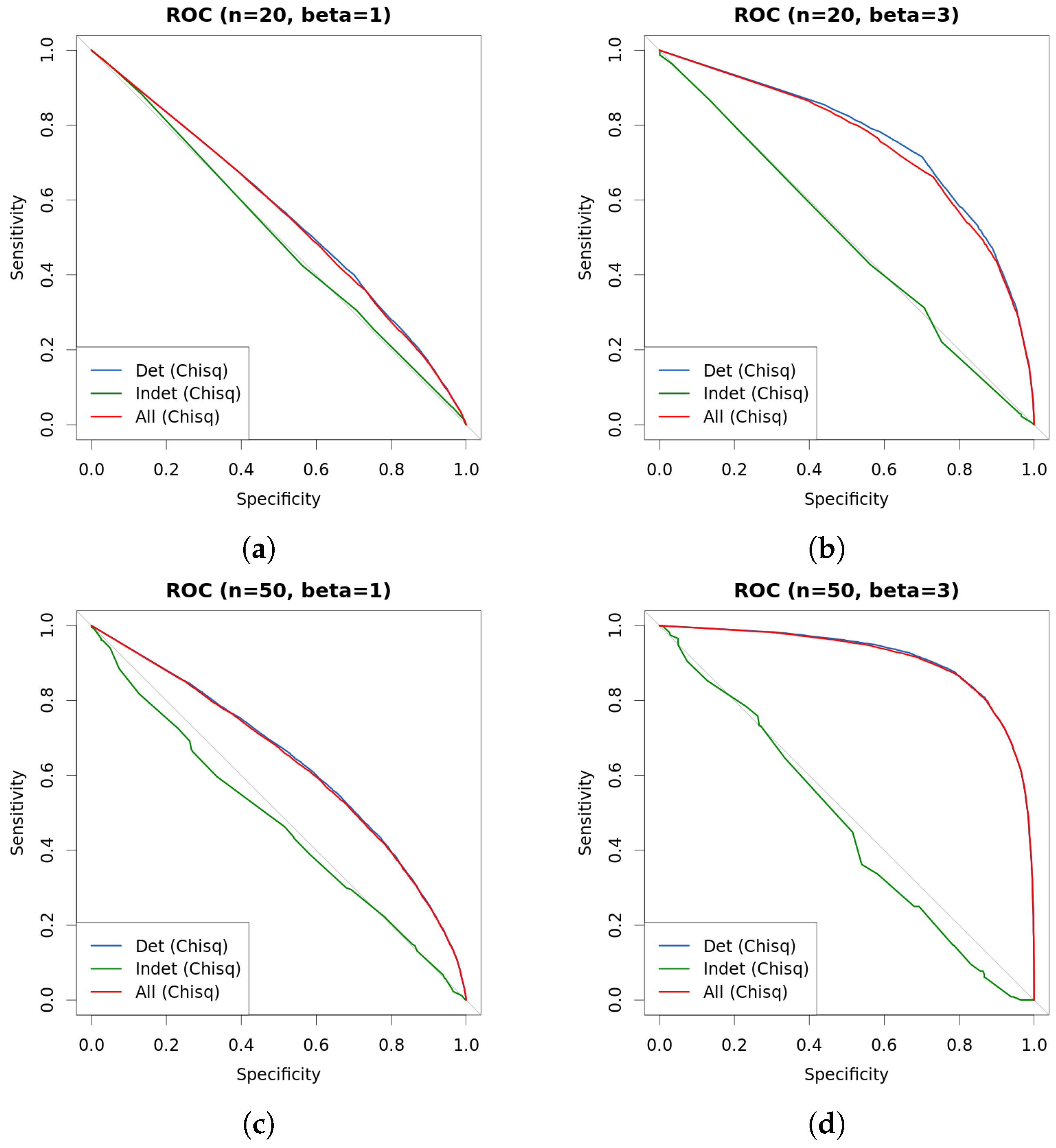
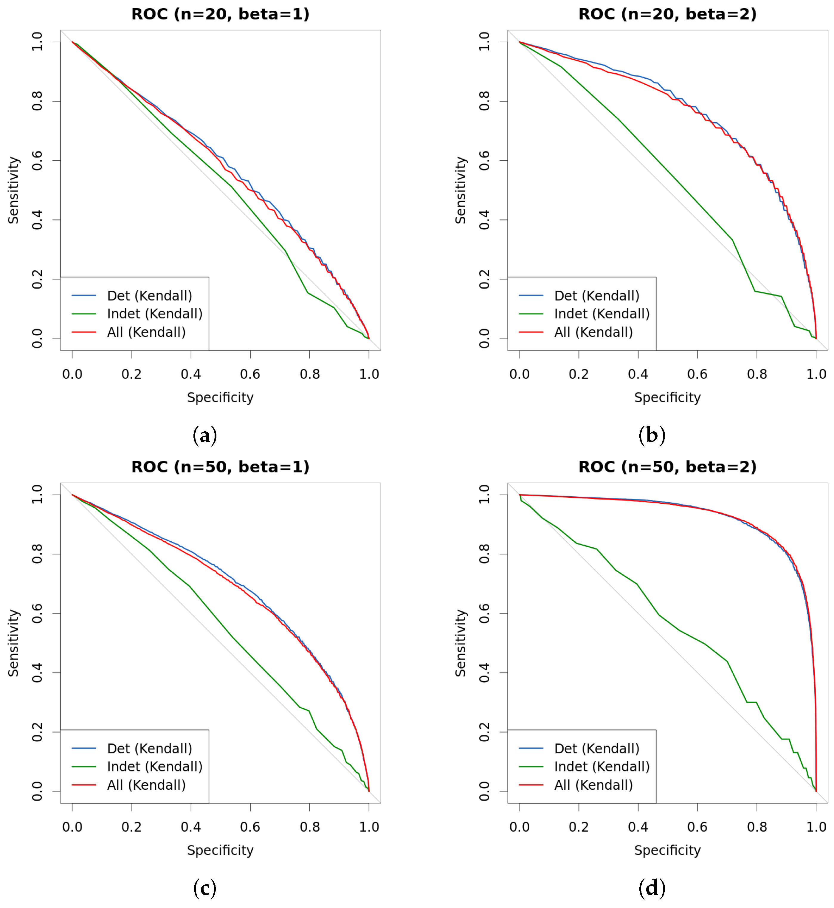
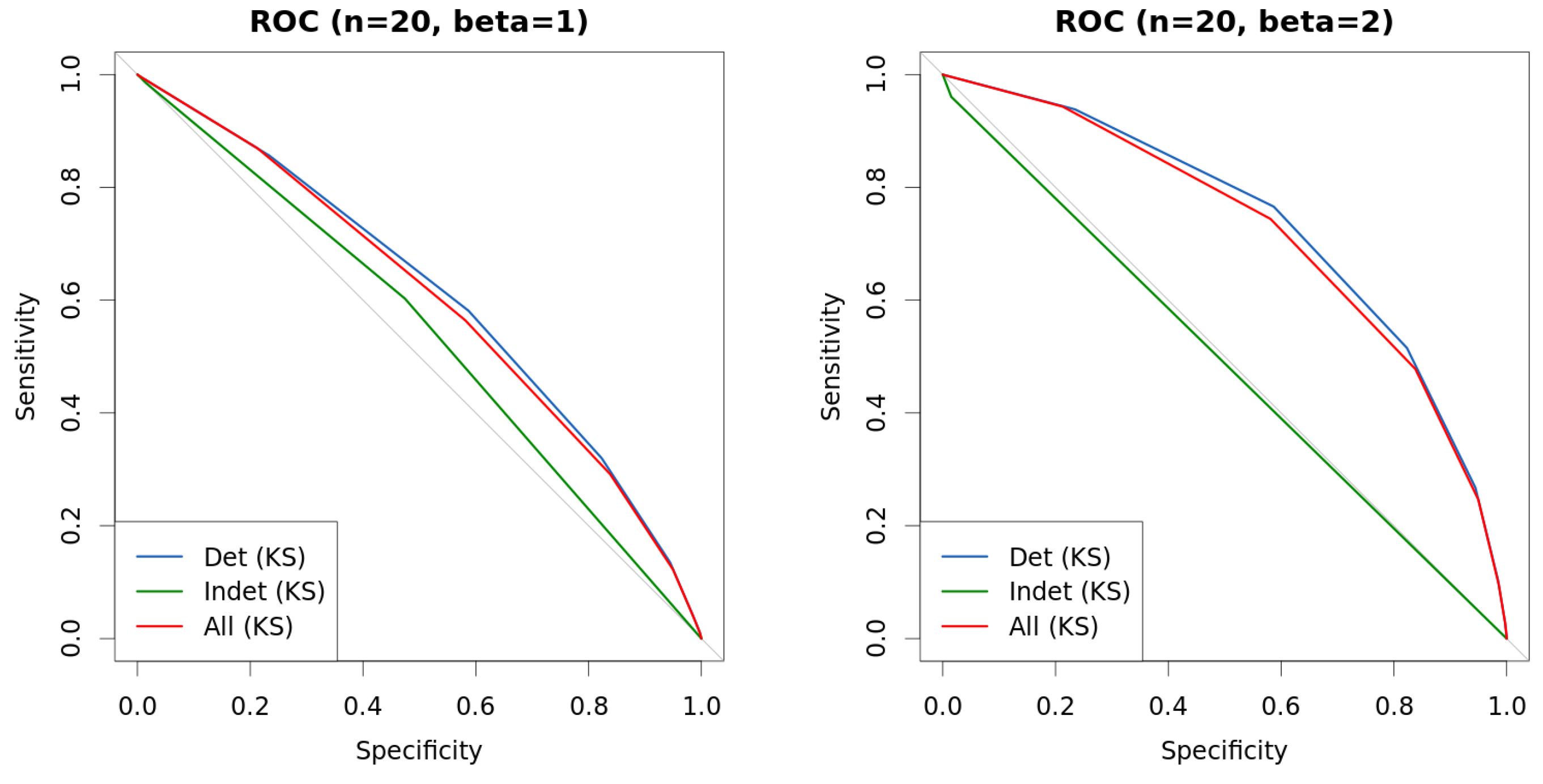
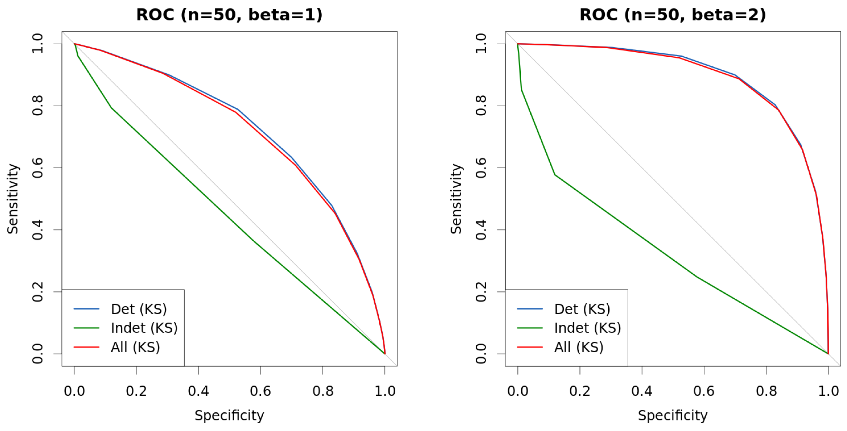
4. Experiments
5. Conclusions
Author Contributions
Conflicts of Interest
Abbreviations
| DP | Dirichlet Process |
| IDP | Imprecise Dirichlet Process |
References
- Raftery, A.E. Bayesian model selection in social research. Sociol. Methodol. 1995, 25, 111–164. [Google Scholar] [CrossRef]
- Goodman, S.N. Toward evidence-based medical statistics. 1: The P–value fallacy. Ann. Intern. Med. 1999, 130, 995–1004. [Google Scholar] [CrossRef] [PubMed]
- Kruschke, J.K. Bayesian data analysis. Wiley Interdiscip. Rev. Cognit. Sci. 2010, 1, 658–676. [Google Scholar] [CrossRef] [PubMed]
- Benavoli, A.; Mangili, F.; Ruggeri, F.; Zaffalon, M. Imprecise Dirichlet Process With Application to the Hypothesis Test on the Probability that X ≤ Y. J. Stat. Theory Pract. 2015, 9, 658–684. [Google Scholar] [CrossRef]
- Benavoli, A.; Mangili, F.; Corani, G.; Zaffalon, M.; Ruggeri, F. A Bayesian Wilcoxon Signed-Rank Test Based on the Dirichlet Process. In Proceedings of the 31st International Conference on Machine Learning (ICML), Beijing, China, 21–26 July 2014; pp. 1026–1034.
- Benavoli, A.; Corani, G.; Mangili, F.; Zaffalon, M. A Bayesian Nonparametric Procedure for Comparing Algorithms. In Proceedings of the 32nd International Conference on Machine Learning (ICML), Lille, France, 6–11 July 2015; pp. 1–9.
- Mangili, F.; Benavoli, A.; de Campos, C.P.; Zaffalon, M. Reliable survival analysis based on the Dirichlet Process. Biom. J. 2015, 57, 1002–1019. [Google Scholar] [CrossRef] [PubMed]
- Kao, Y.; Reich, B.J.; Bondell, H.D. A nonparametric Bayesian test of dependence. 2015; arXiv:1501.07198. [Google Scholar]
- Nandram, B.; Choi, J.W. Bayesian analysis of a two-way categorical table incorporating intraclass correlation. J. Stat. Comput. Simul. 2006, 76, 233–249. [Google Scholar] [CrossRef]
- Nandram, B.; Choi, J.W. Alternative tests of independence in two-way categorical tables. J. Data Sci. 2007, 5, 217–237. [Google Scholar]
- Nandram, B.; Bhatta, D.; Sedransk, J.; Bhadra, D. A Bayesian test of independence in a two-way contingency table using surrogate sampling. J. Stat. Plan. Inference 2013, 143, 1392–1408. [Google Scholar] [CrossRef]
- Friedman, N.; Geiger, D.; Goldszmidt, M. Bayesian network classifiers. Mach. Learn. 1997, 29, 131–163. [Google Scholar] [CrossRef]
- Blum, A.L.; Langley, P. Selection of relevant features and examples in machine learning. Artif. Intell. 1997, 97, 245–271. [Google Scholar] [CrossRef]
- Keogh, E.J.; Pazzani, M.J. Learning Augmented Bayesian Classifiers: A Comparison of Distribution-Based and Classification-Based Approaches. Available online: http://www.cs.rutgers.edu/∼pazzani/Publications/EamonnAIStats.pdf (accessed on 31 August 2016).
- Jiang, L.; Cai, Z.; Wang, D.; Zhang, H. Improving Tree augmented Naive Bayes for class probability estimation. Knowl. Based Syst. 2012, 26, 239–245. [Google Scholar] [CrossRef]
- Ferguson, T.S. A Bayesian Analysis of Some Nonparametric Problems. Ann. Stat. 1973, 1, 209–230. [Google Scholar] [CrossRef]
- Ghosh, J.K.; Ramamoorthi, R. Bayesian Nonparametrics; Springer: Berlin/Heidelberg, Germany, 2003. [Google Scholar]
- Rubin, D.B. Bayesian Bootstrap. Ann. Stat. 1981, 9, 130–134. [Google Scholar] [CrossRef]
- Walley, P. Statistical Reasoning with Imprecise Probabilities; Chapman & Hall: New York, NY, USA, 1991. [Google Scholar]
- Coolen-Schrijner, P.; Coolen, F.P.; Troffaes, M.C.; Augustin, T. Imprecision in Statistical Theory and Practice. J. Stat. Theory Pract. 2009, 3. [Google Scholar] [CrossRef]
- Augustin, T.; Coolen, F.P.; de Cooman, G.; Troffaes, M.C. Introduction to Imprecise Probabilities; John Wiley & Sons: Hoboken, NJ, USA, 2014. [Google Scholar]
- Berger, J.O.; Rios Insua, D.; Ruggeri, F. Bayesian Robustness. In Robust Bayesian Analysis; Insua, D.R., Ruggeri, F., Eds.; Springer: Berlin/Heidelberg, Germany, 2000; Volume 152, pp. 1–32. [Google Scholar]
- Berger, J.O.; Moreno, E.; Pericchi, L.R.; Bayarri, M.J.; Bernardo, J.M.; Cano, J.A.; De la Horra, J.; Martín, J.; Ríos-Insúa, D.; Betrò, B.; et al. An overview of robust Bayesian analysis. Test 1994, 3, 5–124. [Google Scholar] [CrossRef]
- Pericchi, L.R.; Walley, P. Robust Bayesian credible intervals and prior ignorance. Int. Stat. Rev. 1991, 59. [Google Scholar] [CrossRef]
- Dalal, S.; Phadia, E. Nonparametric Bayes inference for concordance in bivariate distributions. Commun. Stat. Theory Methods 1983, 12, 947–963. [Google Scholar] [CrossRef]
- Tan, P.-N.; Steinbach, M.; Kumar, V. Introduction to Data Mining; Pearson Education: New York, NY, USA, 2006. [Google Scholar]
- Jiang, L.; Li, C.; Cai, Z. Learning decision tree for ranking. Knowl. Inf. Syst. 2009, 20, 123–135. [Google Scholar] [CrossRef]
- Jiang, L.; Wang, D.; Zhang, H.; Cai, Z.; Huang, B. Using instance cloning to improve naive Bayes for ranking. Int. J. Pattern Recognit. Artif. Intell. 2008, 22, 1121–1140. [Google Scholar] [CrossRef]
- Robin, X.; Turck, N.; Hainard, A.; Tiberti, N.; Lisacek, F.; Sanchez, J.C.; Müller, M. pROC: An open-source package for R and S+ to analyze and compare ROC curves. BMC Bioinform. 2011, 12. [Google Scholar] [CrossRef] [PubMed]
- Murphy, K.P. Machine Learning: A Probabilistic Perspective; MIT Press: Cambridge, MA, USA, 2012. [Google Scholar]


| Variable 1 | Variable 2 | Distribution |
|---|---|---|
| Binary | Binary | Multinomial distr. with . |
| Continuous | Continuous | Bivariate Gaussian with means 0 and covariance matrix . |
| Binary | Continuous | Half of the samples have the binary variable set to zero and half to one. When that variable is zero, then for the continuous use , otherwise . |
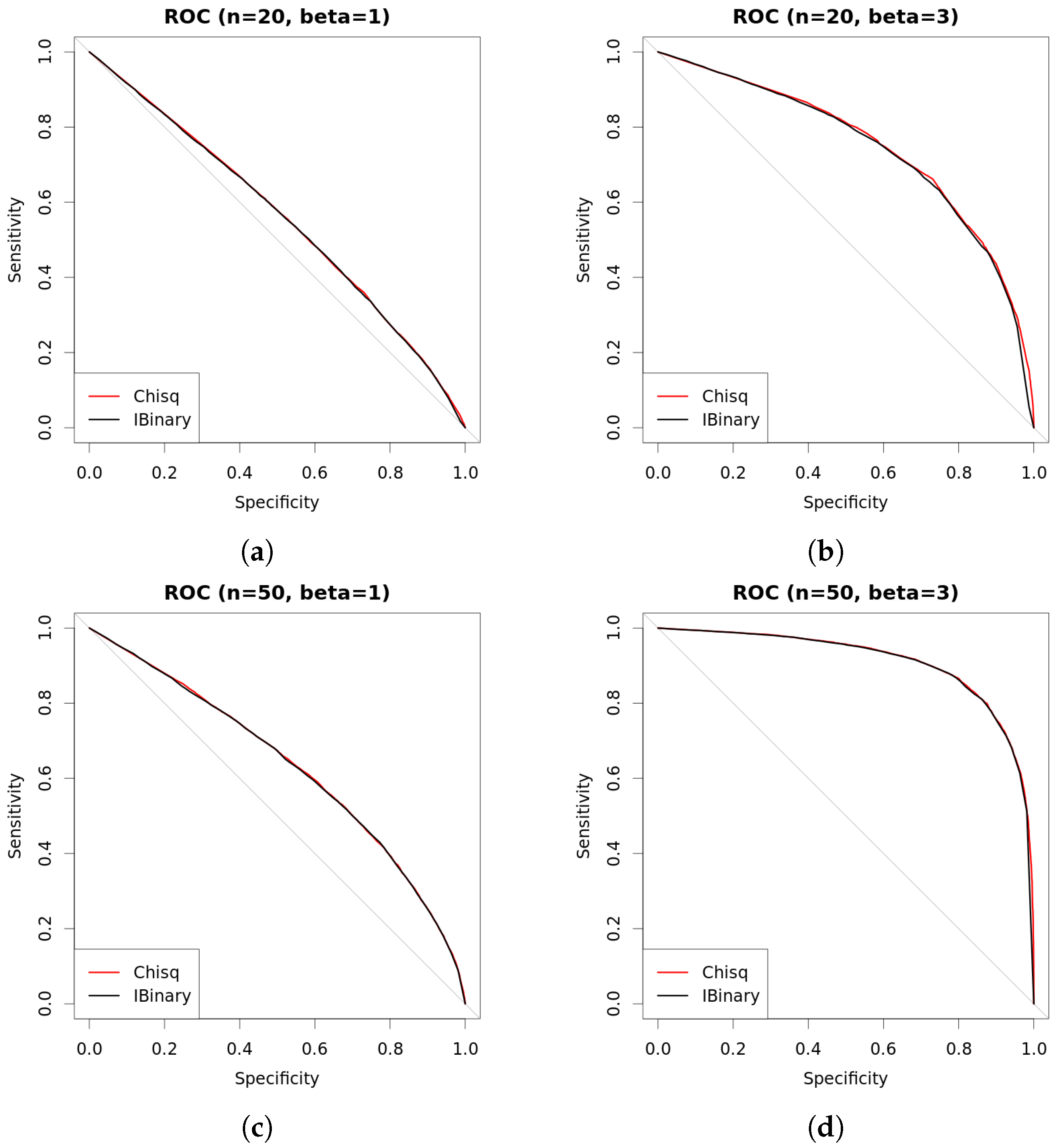
| s | n | β | Chisq | Det.cases | Indet.cases | |
|---|---|---|---|---|---|---|
| 0.25 | 20 | 1 | 0.5562 | 0.5629 | 0.5653 | 0.4890 |
| 0.5 | 20 | 1 | 0.5544 | 0.5596 | 0.5645 | 0.5233 |
| 1 | 20 | 1 | 0.5491 | 0.5551 | 0.5642 | 0.5153 |
| 0.25 | 20 | 3 | 0.7341 | 0.7502 | 0.7567 | 0.4266 |
| 0.5 | 20 | 3 | 0.7388 | 0.7551 | 0.7686 | 0.4526 |
| 1 | 20 | 3 | 0.7330 | 0.7502 | 0.7717 | 0.4888 |
| 0.25 | 50 | 1 | 0.6372 | 0.6425 | 0.6449 | 0.5125 |
| 0.5 | 50 | 1 | 0.6319 | 0.6353 | 0.6393 | 0.4747 |
| 1 | 50 | 1 | 0.6366 | 0.6407 | 0.6492 | 0.4954 |
| 0.25 | 50 | 3 | 0.9145 | 0.9110 | 0.9127 | 0.5205 |
| 0.5 | 50 | 3 | 0.9130 | 0.9090 | 0.9115 | 0.4473 |
| 1 | 50 | 3 | 0.9134 | 0.9081 | 0.9123 | 0.5642 |
| s | n | β | Kendall | Det.cases | Indet.cases | |
|---|---|---|---|---|---|---|
| 0.25 | 20 | 1 | 0.5826 | 0.5858 | 0.5898 | 0.5101 |
| 0.5 | 20 | 1 | 0.5708 | 0.5729 | 0.5804 | 0.4987 |
| 1 | 20 | 1 | 0.5744 | 0.5742 | 0.5914 | 0.5004 |
| 0.25 | 20 | 2 | 0.7524 | 0.7506 | 0.7558 | 0.5037 |
| 0.5 | 20 | 2 | 0.7535 | 0.7502 | 0.7574 | 0.5203 |
| 1 | 20 | 2 | 0.7488 | 0.7407 | 0.7596 | 0.5447 |
| 0.25 | 50 | 1 | 0.6825 | 0.6888 | 0.6917 | 0.5051 |
| 0.5 | 50 | 1 | 0.6782 | 0.6869 | 0.6935 | 0.5633 |
| 1 | 50 | 1 | 0.6871 | 0.6960 | 0.7087 | 0.5204 |
| 0.25 | 50 | 2 | 0.9343 | 0.9191 | 0.9197 | 0.4933 |
| 0.5 | 50 | 2 | 0.9339 | 0.9208 | 0.9207 | 0.5487 |
| 1 | 50 | 2 | 0.9361 | 0.9205 | 0.9192 | 0.5499 |
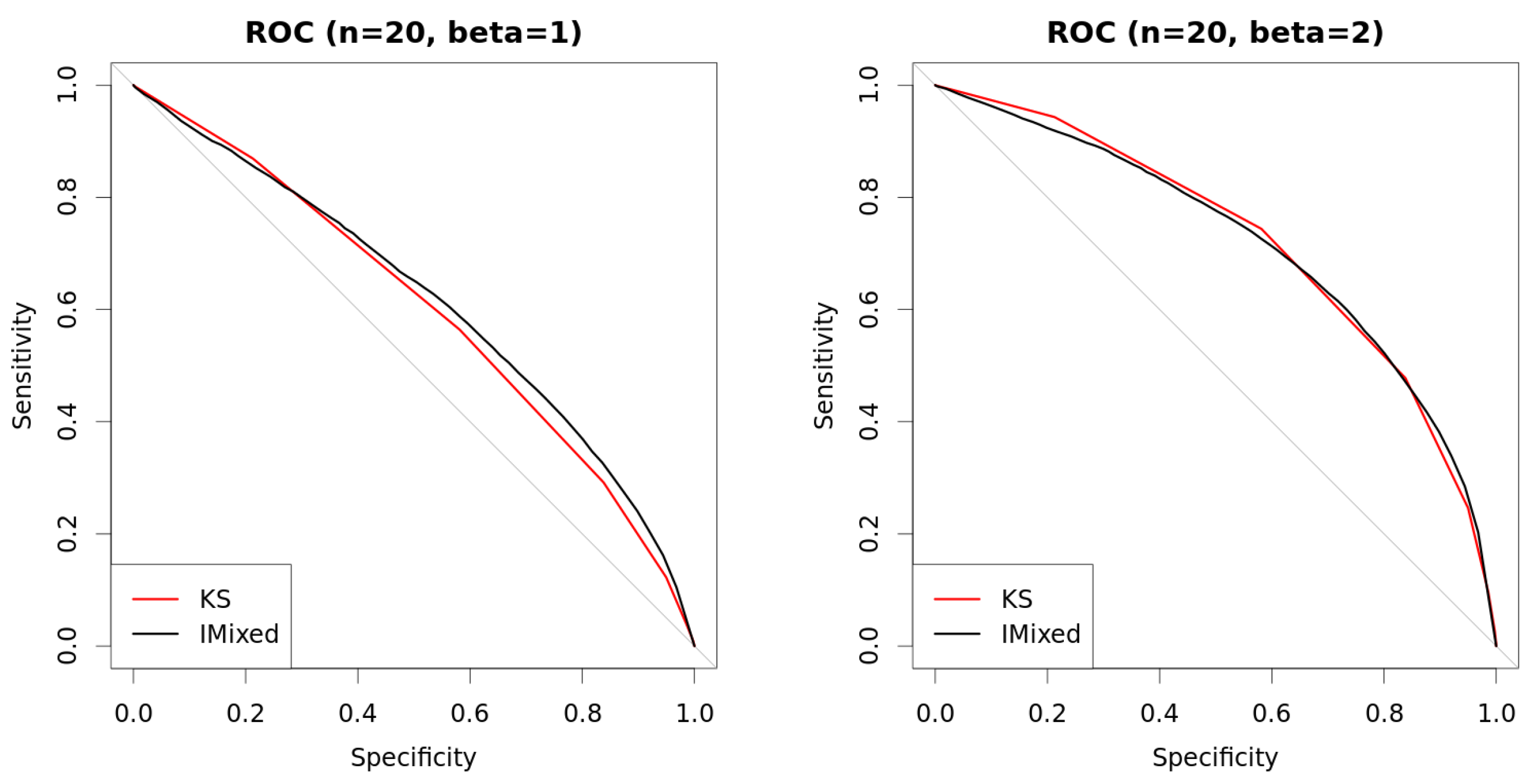
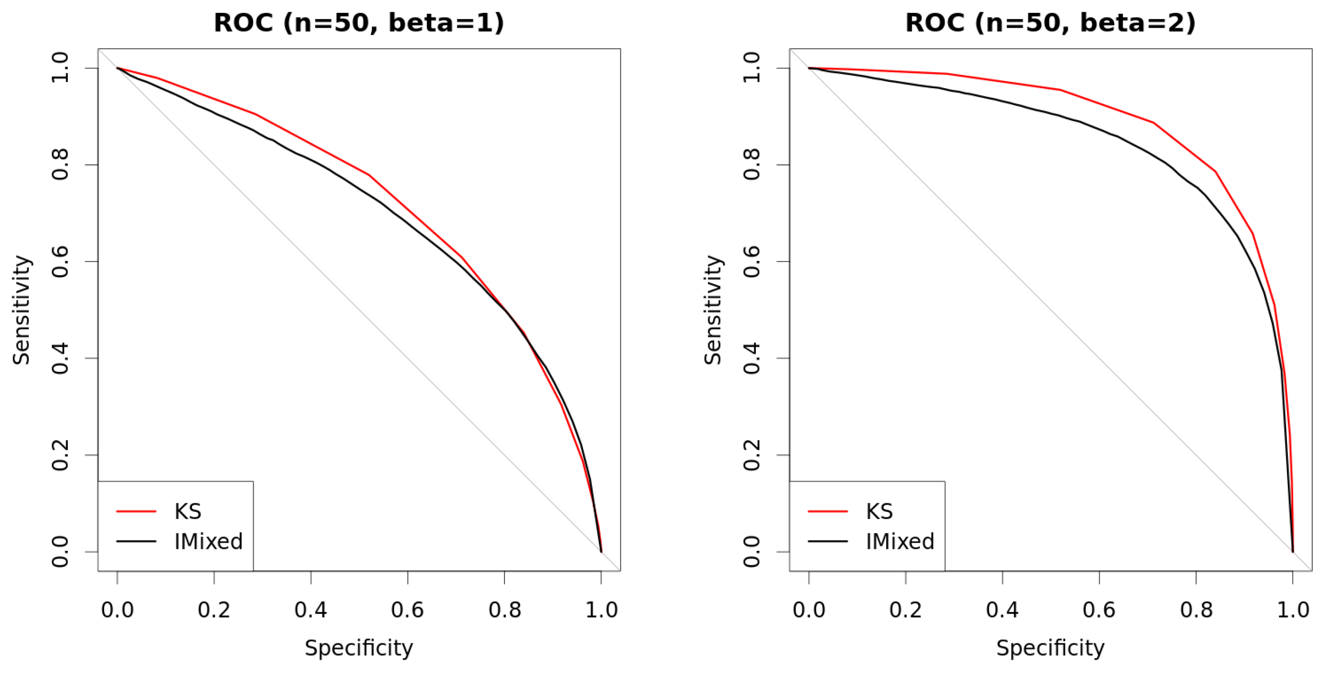
| s | n | β | KS | Det.cases | Indet.cases | |
|---|---|---|---|---|---|---|
| 0.25 | 20 | 1 | 0.6159 | 0.6118 | 0.6139 | 0.5386 |
| 0.5 | 20 | 1 | 0.6150 | 0.5943 | 0.5989 | 0.5594 |
| 1 | 20 | 1 | 0.6132 | 0.6004 | 0.6104 | 0.5532 |
| 0.25 | 20 | 2 | 0.7176 | 0.7358 | 0.7392 | 0.5254 |
| 0.5 | 20 | 2 | 0.7202 | 0.7091 | 0.7159 | 0.4937 |
| 1 | 20 | 2 | 0.7163 | 0.7091 | 0.7233 | 0.4928 |
| 0.25 | 50 | 1 | 0.6997 | 0.7091 | 0.7109 | 0.4447 |
| 0.5 | 50 | 1 | 0.6966 | 0.7106 | 0.7149 | 0.4213 |
| 1 | 50 | 1 | 0.7076 | 0.7135 | 0.7224 | 0.4455 |
| 0.25 | 50 | 2 | 0.8526 | 0.8816 | 0.8832 | 0.3278 |
| 0.5 | 50 | 2 | 0.8497 | 0.8790 | 0.8818 | 0.3044 |
| 1 | 50 | 2 | 0.8562 | 0.8923 | 0.8986 | 0.2934 |
© 2016 by the authors; licensee MDPI, Basel, Switzerland. This article is an open access article distributed under the terms and conditions of the Creative Commons Attribution (CC-BY) license (http://creativecommons.org/licenses/by/4.0/).
Share and Cite
Benavoli, A.; De Campos, C.P. Bayesian Dependence Tests for Continuous, Binary and Mixed Continuous-Binary Variables. Entropy 2016, 18, 326. https://doi.org/10.3390/e18090326
Benavoli A, De Campos CP. Bayesian Dependence Tests for Continuous, Binary and Mixed Continuous-Binary Variables. Entropy. 2016; 18(9):326. https://doi.org/10.3390/e18090326
Chicago/Turabian StyleBenavoli, Alessio, and Cassio P. De Campos. 2016. "Bayesian Dependence Tests for Continuous, Binary and Mixed Continuous-Binary Variables" Entropy 18, no. 9: 326. https://doi.org/10.3390/e18090326