Abstract
The detectability for a noise-enhanced composite hypothesis testing problem according to different criteria is studied. In this work, the noise-enhanced detection problem is formulated as a noise-enhanced classical Neyman–Pearson (NP), Max–min, or restricted NP problem when the prior information is completely known, completely unknown, or partially known, respectively. Next, the detection performances are compared and the feasible range of the constraint on the minimum detection probability is discussed. Under certain conditions, the noise-enhanced restricted NP problem is equivalent to a noise-enhanced classical NP problem with modified prior distribution. Furthermore, the corresponding theorems and algorithms are given to search the optimal additive noise in the restricted NP framework. In addition, the relationship between the optimal noise-enhanced average detection probability and the constraint on the minimum detection probability is explored. Finally, numerical examples and simulations are provided to illustrate the theoretical results.
1. Introduction
Stochastic resonance (SR) is a phenomenon where the performance of a nonlinear system can be enhanced by the presence of noise under certain circumstances. The concept of SR was first brought up by Benzi et al. in the process of exploring the periodic recurrence of ice gases [1] and since then the positive effects of noise have increasingly attracted researchers’ attention in various fields, such as physics, chemistry, biology, and electronics [2,3,4,5,6,7,8,9]. The performance boost of a noise-enhanced system has also been observed in numerous signal detection problems; for example, when adjusting the background noise level or injecting additive noise to the input, the output of the system can be improved in some cases [10,11,12,13,14,15]. The improvements obtained via noise can be measured by various metrics, such as an increase in mutual information (MI) [16,17,18,19], output signal-to-noise ratio (SNR) [20,21,22], or detection probability [23,24,25,26,27,28,29], or a decrease in Bayes risk [30,31,32] or error probability [33].
For the hypothesis testing problem [34], the optimal additive noise to improve the performance of a suboptimal detector is usually determined according to Bayesian [24,25], Minimax [30], and Neyman–Pearson (NP) [23,24,25,26] criteria. For example, the minimization of Bayes risk obtained by adding additive noise to the observation has been investigated based on Bayesian criteria under the uniform cost assignment in [33], and it is proven that the optimal additive noise to minimize the error probability is a constant vector. According to the NP criteria, the maximization of detection probability obtained by adding additive noise has been considered under the constraint on the false-alarm probability. In [23], the detection of a direct current (DC) signal embedded in independent and identically distributed (i.i.d.) Gaussian mixture noise is studied, which illustrates that the detection probability of a suboptimal detector can be increased by adding an independent additive noise to the received data. In [24], a mathematical framework for the noise-enhanced binary hypothesis testing problem is formulated according to the NP criterion. The optimal noise is proven to be a randomization of no more than two discrete vectors and sufficient conditions for the increase of the detection probability via additive noise are also provided. Theorems and algorithms are also provided in [26] to search for the optimal or near-optimal SR noise that benefits the NP and inequality-constrained signal detection problems.
Composite hypothesis testing problems are often encountered in practical applications, for example, radar systems, spectrum sensing in cognitive radio networks, and non-coherent communication receivers [35,36]. In such problems, there are multiple parameters with different probabilities under each alternative hypothesis [27]. Therefore, noise that benefits composite hypothesis testing problems can also be investigated according to Bayesian, Minimax, and NP criteria. If the prior information of each parameter is completely available, the noise-enhanced Bayesian and NP approaches can be utilized. When no prior information exists, it is appropriate to select the Minimax approach to find the optimal additive noise.
Nevertheless, due to the existence of estimation error, prior information usually has some uncertainties [34]. For instance, in some cases, only part of the prior information can be utilized [37]. Accordingly, the classical Bayesian, Minimax, and NP criteria are not suitable in such cases, and a more restricted criterion should be considered in order to utilize the available partial prior information adequately. In [31], under certain constraints of the conditional risks, the optimal noise to minimize the Bayes risk is explored according to the restricted Bayesian criterion. Generally, the constraint is determined on the basis of the uncertainty in the prior information. Actually, the noise-enhanced composite hypothesis testing problem in the restricted Bayesian framework can be generalized to the Bayesian framework and Minimax framework simply by changing the value of the constraints.
In [27], the restricted NP criterion is used to find the optimal decision rule for the composite hypothesis testing problem, which focuses on maximizing the average detection probability under the constraints that the minimum detection probability cannot be less than a predefined value and the maximum false-alarm probability cannot be larger than a given level. In this way, since the constraint on the minimum detection probability is adjusted according to the uncertainty in the prior information, it not only ensures the detection probability in the worst case, but also uses the prior information effectively. Furthermore, the classical NP and Max–min criteria are special cases of the restricted NP criterion. The former aims to maximize the average detection probability based on the prior distribution with the constraint on false-alarm probability, and the latter focuses on the maximization of the minimum detection probability under the same constraint on false-alarm probability. For the case where the decision rule cannot be altered, the restricted NP criterion can also be employed to investigate the optimal additive noise for the composite hypothesis testing problem (see the study in [29]).
Inspired by the studies in [27,29], the main focus of this work is to find the relations of the optimal additive noises obtained under restricted NP criterion and classical NP criterion with different prior distributions in which the noise-enhanced detection problem for composite hypothesis testing can be solved more thoroughly. In addition, the links of the average and minimum detection probabilities based on the noise-enhanced restricted NP, classical NP, and Max–min approaches are also discussed.
Our main contributions are summarized as follows. First, the noise enhanced composite hypothesis-testing problem is formulated according to the classical NP, Max–min, or restricted NP criterion when the prior information is completely known, completely unknown, or partially known, respectively. Then the detection performances obtained under different criteria are compared and the feasible range of the constraint on the minimum detection probability is provided. Further, under certain conditions, a special conclusion is made that the noise-enhanced restricted NP problem is equivalent to a noise-enhanced classical NP problem with a modified prior distribution and using the same constraint on the false-alarm probability. Based on this conclusion, theorems and algorithms are presented to find the optimal noise in the restricted NP framework. In addition, the relationship between the optimal noise-enhanced average detection probability and the constraint on the minimum detection probability is also explored.
Remarkably, the results in this paper can be directly applied in some specific physical environments. For instance, in order to detect a sinusoidal signal embedded in noise through exploiting the escape time of a Josephson junction [8], the escape time is regarded as the observation and the corresponding probability distribution functions (PDFs) under two hypotheses are retrieved by utilizing various nonparametric statistical techniques, such as the kernel density estimation (KDE). Generally, the distributions of the signal parameters are known with some uncertainties due to the estimation errors. In such a case, the restricted NP approach developed in this paper can be utilized. In addition, if we assume the signal parameters are completely known or unknown, the classical NP or Max–min approach can be employed, respectively, to find the corresponding noise that will enhance system performance.
The remainder of this paper is organized as follows. In Section 2, the noise-enhanced binary composite hypothesis testing problems are formulated according to the classical NP, Max–min, and restricted NP criteria, and the corresponding detection performances are compared. In Section 3, the theorems and algorithms necessary to find the modified prior distribution and the optimal additive noise are developed. In addition, some characteristics of maximum noise-enhanced average detection probability obtained in restricted NP approach are also discussed. Finally, numerical examples and simulations are presented in Section 4 to illustrate the theoretical results, and conclusions are drawn in Section 5.
2. Noise-Enhanced Detection
2.1. Problem Formulation
Consider a classical binary composite hypothesis testing problem, given by
where represents the PDF of the observation for a given parameter , is a N-dimensional vector and . In addition, and are the sets of all possible values of parameter under and , respectively, and . The union of the two sets forms the parameter space , i.e., . The PDF for the parameter under , , is denoted by .
Studies have shown that the detection performance of a system can be improved by adding an independent additive noise to the observation for the case where the detector cannot be varied. The corresponding noise modified observation is denoted by
The PDF of for a given parameter can be expressed as
where denotes the PDF of the additive noise . Using Equation (3), the noise-modified detection and false-alarm probabilities for given parameter values are respectively defined as
where is the decision rule of the detector and also indicates the probability of choosing . Due to the fact that the detector is fixed, the decision rule for the noise-modified observation is the same as that for . For the case where the detector is fixed, one reasonable way to improve the detectability of the system is to optimize the additive noise.
2.2. Noise-Enhanced Detection Problems under Different Criteria
For noise-enhanced composite hypothesis testing problems, the general means is to search for the optimal additive noise to improve the system performance according to the classical NP criterion, which requires that the noise modified false-alarm probability for any possible values of parameter in the set should be below a certain constraint and the noise-modified average detection probability should reach the achievable maximum. In such a case, there is no link between the PDF of under , i.e., , and the optimal additive noise. On the other hand, the solution of the optimal additive noise is closely related to the PDF of under , i.e., .
When is completely known, the optimal additive noise is usually explored according to the classical NP criterion, which is formulated by
where represents the PDF of the optimal additive noise obtained by the noise-enhanced classical NP approach, represents the noise-enhanced average detection probability based on the estimated prior probability , and is the upper limit for the false-alarm probability.
When is completely unknown, the optimal additive noise can be determined based on the Max–min criterion, where the minimum noise enhanced detection probability is maximized under the constraint on the false-alarm probability. The corresponding noise enhanced problem can be expressed by
where denotes the optimal additive noise PDF in the noise enhanced Max–min approach.
In practice, is usually estimated according to previous experience and estimation errors are unavoidable, leading to some uncertainties in . The existence of the estimation error is often ignored when the noise enhanced detection problem based on the NP criterion is investigated. Once the Max–min criterion is applied, the previous experience cannot be utilized effectively. Therefore, it is not a suitable method for finding the optimal additive noise according to the NP criterion or the Max–min criterion directly when there are uncertainties in . In order to utilize previous experience and consider the uncertainty in estimation simultaneously, the restricted NP criterion proposed in [27] is utilized in this paper. Based on the estimated distribution , the noise-enhanced restricted NP approach seeks to maximize average detection probability by adding appropriate noise, under the constraints that the minimum detection probability stays above a certain value and the maximum false-alarm probability stays below a certain level. It should be noted that the constraint on the minimum detection probability can be adjusted depending on the degree of the uncertainty. As a result, the noise-enhanced problem according to the restricted NP criterion is formulated as follows:
where denotes the optimal additive noise PDF in the noise-enhanced restricted NP approach, is the lower limit for detection probability, and an appropriate is chosen according to the uncertainty in . Generally, is chosen as , where and represents the Max–min detection probability obtained in the noise-enhanced Max–min approach, i.e., .
When the prior information about is completely unknown, we set and the noise-enhanced detection problem in the restricted NP framework is reduced to that in the Max–min framework. When is completely known, we set and the noise-enhanced detection problem in the restricted NP framework becomes the noise-enhanced problem in the classical NP framework. As a result, the noise-enhanced Max–min problem and classical NP problem can be regarded as two special cases of the noise-enhanced restricted NP problem.
2.3. Analysis on the Noise-Enhanced Detectability
In this subsection, the relationships among the different noise-enhanced approaches are clarified in detail. We first compare the detection performances obtained via additive noise under different criteria and then determine the feasible range of , which is the lower limit of the detection probability for any .
In the noise-enhanced restricted NP framework, the maximization of the average detection probability needs to consider the constraints on the minimum detection probability for and the maximum false-alarm probability for simultaneously. On the other hand, the aim of the noise-enhanced classical NP problem is to find the additive noise that maximizes the average detection probability with only the constraint on false-alarm probability, while ignoring any constraints on the minimum detection probability. Generally speaking, the maximum average detection probability obtained by the noise-enhanced restricted NP approach is less than or equal to that obtained by the noise-enhanced classical NP approach, and the minimum detection probability obtained by the noise-enhanced restricted NP approach is greater than or equal to that obtained by the noise-enhanced classical NP approach. For the noise enhanced Max–min approach, however, the aim is to search the additive noise that achieves the maximum of the minimum detection probability under the constraint on false-alarm probability. Therefore, the minimum detection probability obtained by the noise-enhanced Max–min approach is greater than or equal to that obtained by the noise enhanced restricted NP approach.
Based on the discussions above, in what follows, the detectability in the noise-enhanced restricted NP framework is analyzed when takes different values. From the definitions given in Section 2.2, , , and are the optimal additive noise PDFs corresponding to the noise-enhanced restricted NP, classical NP, and Max–min approaches, respectively. In order to facilitate the analysis that follows, we define
i.e., and are the minimum detection probabilities corresponding to the noise-enhanced classical NP approach and Max–min approach for , respectively.
If , the noise-enhanced restricted NP problem is simplified to the noise enhanced classical NP problem. It is obvious that the constraint enforced by is ineffective in this case. Accordingly, the optimal additive noise and the maximum noise-modified average detection probability obtained by the restricted NP approach are the same as those obtained by the classical NP approach, i.e., and . Furthermore, based on the formulation of the noise enhanced Max–min approach, is the achievable maximum of the minimum detection probability for any obtained by adding additive noise under the constraint on false-alarm probability. Therefore, there are no additive noises that satisfy the condition of . In other words, it is not suitable to set . As a result, the value of should be selected in the interval , otherwise the constraint on the minimum detection probability will be meaningless.
3. Optimal Additive Noises in Restricted NP and Classical NP Frameworks
In this section, we shall further explore the connections implied in the optimal additive noises obtained by the restricted NP and classical NP approaches under certain conditions. The related characteristics are discussed in order to develop an algorithm that determines the optimal additive noise under the restricted NP framework. For the convenience of discussions, we define
With these notations, the optimization problem in (10) and (11) can be reformulated as
Actually, the problem in Equations (16) and (17) can be expressed in alternative form as follows:
where is a parameter selected depending on and .
3.1. Characteristics of the Optimal Additive Noise
According to Equations (18) and (19), Theorem 1 shows some characteristics of the optimal additive noise obtained by the restricted NP approach.
Theorem 1.
Define a PDF of under as , where is any valid PDF. If there exists a PDF such that
where is the optimal additive noise PDF that maximizes the average detection probability based on under the constraint that , then is the optimal solution of Equations (18) and (19). The proof is presented in Appendix A.
Theorem 1 implies that the solution of the noise-enhanced restricted NP problem is the same as that of a noise-enhanced classical NP problem under certain conditions. Specifically, if there exists a PDF that satisfies the condition in Equation (20), the noise-enhanced restricted NP problem shown in (18) and (19) is equivalent to the noise-enhanced classical NP problem based on the probability distribution of under , denoted by . As discussed above, the definition of can be formulated as
The form of the optimal additive noise PDF is proven as a randomization of no more than discrete vectors and the corresponding algorithm has been provided in [28], where is the number of in the set .
The following corollary shows the link between the optimization noise-enhanced problem in Equations (18) and (19) and that in (10) and (11).
Corollary 1.
Under the conditions in Theorem 1, if , is the optimal additive noise PDF corresponding to the optimization problem described in Equations (10) and (11). The proof is omitted here and provided in Appendix A.
First, Corollary 1 illustrates that is the solution of the optimization problem described in Equations (16) and (17), or the one in (10) and (11), when the additive noise PDF in Theorem 1 satisfies . In such a case, when the noise-modified average detection probability based on reaches the achievable maximum, the corresponding minimum detection probability for all is equal to . Second, for any , the corresponding can be calculated based on the equality in Corollary 1.
In addition, in order to find , we first define a family of ’s PDF of the following form:
where and represent the weights of and in , respectively, , and is any valid PDF. Theorem 2 below states a conclusion that in Theorem 1 is the PDF corresponding to the minimum noise-enhanced average detection probability, which is among the family of PDFs with the form of .
Theorem 2.
Under the conditions in Theorem 1, is the PDF that minimizes the noise-modified average detection probability among all probability distributions of the form , where , , and is any PDF. In other words, the following inequality holds:
where and are the optimal additive noise PDFs obtained by the classical NP approach corresponding to and , respectively. The proof is omitted here and provided in Appendix A.
Obviously, is a special case of , and therefore we can search the explicit expression of and the optimal additive noise under the restricted NP criterion by exploiting the conclusion in Theorem 2. In addition, since is a special value of , for practical applications we only need to consider the case of . The detailed algorithm is presented in the next subsection.
3.2. Algorithm for the Optimal Additive Noise
The analysis in Subsection 3.1 indicates that, in order to solve the noise-enhanced restricted NP problem in Equations (10) and (11), we need to obtain a distribution and the optimal additive noise PDF corresponding to in the classical NP framework to satisfy the conditions in Theorem 1. To achieve this aim, the condition of (20) in Theorem 1 is rewritten as
Equation (25) reveals that only assigns nonzero values where corresponds to the global minimum of . It is assumed that the value of that achieves the global minimum of is unique and thus can be expressed as
where represents the unique that minimizes . Based on this assumption, the following algorithm is provided to find and .
| Algorithm 1 Optimal Additive Noise in the Restricted NP Approach |
| (1) Obtain for all , where represents the optimal additive noise corresponding to in the classical NP framework under the constraint of . |
| (2) Calculate , and solve the following minimization problem:
|
| (3) If , is the solution of the noise-enhanced restricted NP problem in Equations (10) and (11). Otherwise, there is no optimal solution. |
In Algorithm 1, can be regarded as the average detection probability corresponding to and Step (2) is satisfied based on Theorem 2. It should be noted that the obtained in Equation (27) may be not unique. When that happens, for any and if the corresponding optimal additive noise satisfies the equality in Step (3), is the solution of the noise-enhanced restricted NP problem, according to Theorem 1.
If there is more than one value of corresponding to the global minimum , the expression of can be written as
where , , and are the value and the number of corresponding to the global minimum , respectively. In such a case, let represent the vector consisting of all the unknown parameters in , i.e., . Accordingly, Step (2) in the algorithm can be updated by
where denotes the optimal additive noise PDF corresponding to obtained by the noise-enhanced classical NP approach. Moreover, if the condition of in Step (3) holds, the corresponding is indeed the solution of Equations (10) and (11). From the analysis above, compared to the case where the global minimum of is achieved by a unique , the computational complexity is increased significantly. In order to overcome this problem, some global optimization algorithms, for example the ant colony algorithm (ACO), genetic algorithm (GA), and particle swarm optimization algorithm (PSO), can be utilized to find .
If there are infinite values of that achieve the global minimum , the Parzen window density estimation can be used to approximate the form of that solves the noise-enhanced restricted NP problem. Specifically, can be approximately denoted by a convex combination of multiple window functions, given by
The noise-enhanced restricted NP problem can now be solved by updating the algorithm through replacing with and redefining as the optimal additive noise corresponding to obtained by the noise-enhanced classical NP approach.
In practical applications, the value and number of to maximize are generally unknown in advance. Therefore, we usually first assume that there exists only one corresponding to the global minimum , and then can be solved according to the Algorithm 1. If the result matches the condition in Step (3), the noise-enhanced restricted NP problem in Equations (10) and (11) has been solved. Otherwise, according to the algorithm and in order to solve the global minimum, the number of values of will be incrementally increased until the optimal noise that satisfies the noise-enhanced restricted NP criterion is obtained.
3.3. Noise-Enhanced Average Detection Probability on β
As concluded in Section 2.2, is ineffective for and meaningless for . Therefore, in the rest of this section we shall only consider the noise-enhanced average detection probability obtained under the restricted NP framework for . Prior to discussing the relation between and for , an important concept should be explained explicitly first, namely, that for any we have
We now employ the contradiction method to illustrate the conclusion in Equation (31). It is assumed that . In this case, there exists an additive noise PDF , , that satisfies , where is the optimal additive noise PDF in the noise-enhanced classical NP approach. According to the definition of , and . Consequently, , which contradicts the definition of . Therefore, the minimum of for cannot be greater than , i.e., . Theorem 3 now shows the link between and , .
Theorem 3.
When , the maximum noise-modified detection probability obtained by the restricted NP approach is a strictly decreasing and concave function of . The proof is presented in Appendix A.
Theorem 3 illustrates that the maximum noise-enhanced average detection probability increases monotonically as decreases towards . In other words, the average detection probability can be improved by reducing the constraint on the minimum detection probability in practical applications. On the other hand, is chosen according to the estimation uncertainty. When the uncertainty decreases, we can select a smaller . Therefore, Theorem 3 also indicates that the higher the validity of estimation, the greater the average detection probability that could be obtained by adding additive noise.
4. Numerical Examples and Simulation Analysis
In this section, the conclusions investigated in the previous sections will be verified through a practical example and the corresponding simulations. The two hypotheses are considered here and given by
where , is a parameter with some uncertainties, and is a symmetric Gaussian mixture noise with the PDF of form
where , , and . In this example, the parameter is modeled as a random variable with the PDF
where is a known positive constant, and is known, but with some uncertainties. The sets of under and are and , respectively. The conditional PDF of for any given value of can be calculated by
The decision rule of the detector is given as
where and denotes the independent additive noise. Correspondingly,
where .
In this example, let and suppose that the means of the symmetric Gaussian components in the mixture noise are [0.1 0.6 −0.6 −0.1], with corresponding weights of [0.35 0.15 0.15 0.35]. In addition, it is assumed that the variances of the symmetric Gaussian components in the mixture noise are the same, namely for . From the analysis in Section 3.2, we assume first, and then the algorithm presented in Equation (28) can be utilized to find and the corresponding optimal additive noise. If the solution satisfies the condition in Step (3), the optimal additive noise is obtained by the restricted NP approach. Otherwise, it should be assumed that , where . In this case, we only need to utilize the algorithm to determine the unknown parameter , which minimizes the average detection probability based on the prior distribution , and the optimal additive noise can be obtained accordingly.
Figure 1 compares the maximum noise-modified average detection probabilities obtained by the restricted NP approach versus for , , and when , , and . Due to the symmetry of the background noise, the original average detection probability is independent of and equals 0.8878. Compared with the data in Figure 1, the average detection probability can be improved by adding additive noise under the constraints that the false-alarm probability should not be greater than and the minimum detection probability should not be less than . As defined in Equation (12), the three values of , i.e., , , and , in Figure 1 are the minimum detection probabilities obtained by the noise-enhanced classical NP approach for , and , respectively. In this example, the value of increases with the decrease of , i.e., . From Figure 1, is the minimum detection probability obtained by the noise enhanced Max–min approach. At the same time, is the achievable maximum of the minimum detection probability in the three different noise-enhanced approaches, which is consistent with the definition given in Equation (13). Additionally, the value of is independent of and .
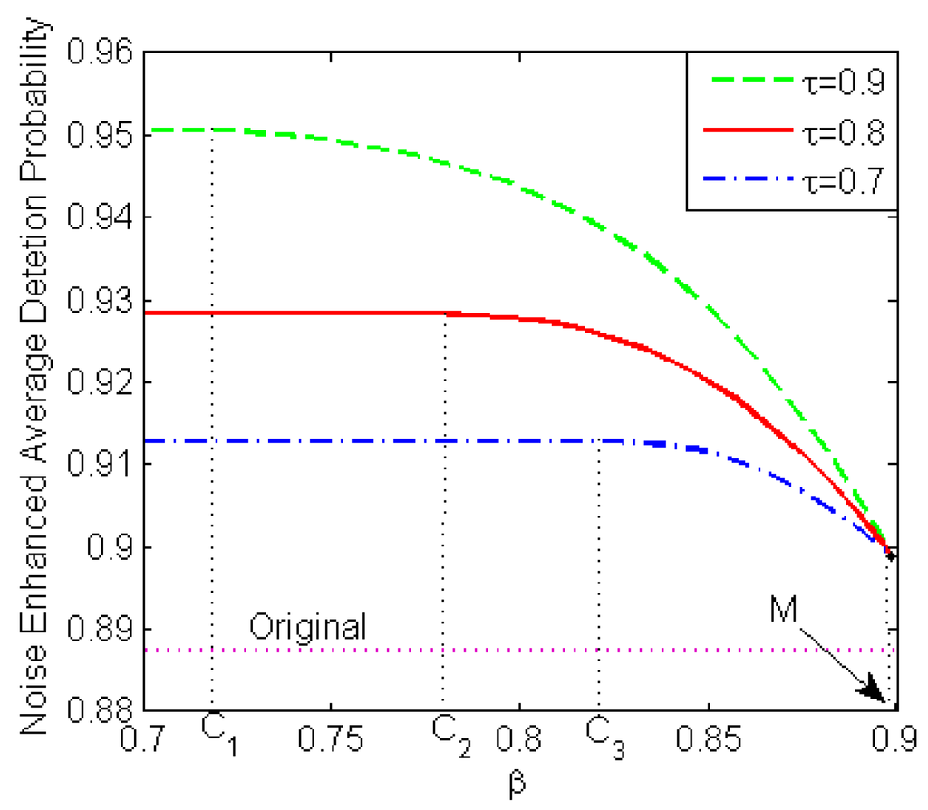
Figure 1.
Noise-enhanced average detection probabilities versus obtained by the restricted NP approach for , and when , , and .
With the decrease of , the maximum noise-modified average detection probability obtained by the restricted NP approach decreases, and the corresponding value of increases and approaches . When , both the noise-enhanced restricted NP problem and the noise-enhanced classical NP problem are equivalent to the noise-enhanced Max–min problem. If for a given , the maximum noise-modified average detection probability obtained by the restricted NP approach decreases with the increase of . If , the optimal solution for the noise-enhanced restricted NP problem is the same as that for the noise-enhanced classical NP problem. Therefore, the maximum noise-modified average detection probability obtained by the restricted NP approach remains constant for and is equal to that obtained by the noise-enhanced classical NP approach.
Figure 2 depicts the maximum noise-enhanced average detection probabilities and the corresponding minimum detection probabilities versus obtained by the restricted NP approach for , , and when , , and . As shown in Figure 2, for a given value of , when the value of exceeds a certain threshold , the maximum noise-enhanced average detection probability increases and the corresponding minimum detection probability decreases with an increase of . According to the analysis in the previous sections, the value of is specified by . When , the noise-enhanced restricted NP problem is equivalent to the noise-enhanced Max–min problem, and the corresponding maximum noise-enhanced average detection probability is the same as the minimum detection probability, and equal to . In this case, the value of is independent of , which also agrees with the conclusion in Figure 1. In addition, the value of decreases as increases, shown in Figure 2, namely , where , , and are the values of corresponding to , , and , respectively. In other words, a larger provides a bigger feasible range of . In general, the maximum noise-enhanced average detection probability obtained by the restricted NP approach increases, while the corresponding minimum detection probability decreases with an increase of for any .
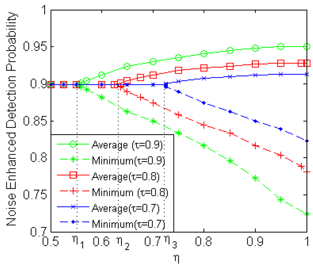
Figure 2.
Noise-enhanced average and minimum detection probabilities versus obtained by the restricted NP approach for , , and when , , and .
Figure 3 illustrates the average detection probabilities for and 0.35 obtained by the noise-enhanced restricted NP approach and the original detector versus when , and . It is seen that with the increase of the original average detection probability initially remains constant, then decreases gradually after reaching the maximum. On the other hand, the average detection probability obtained by the noise-enhanced restricted NP approach initially remains constant then gradually decreases. In addition, the smaller the value of , the greater the gain obtained by adding noise. Compared with the average detection probabilities obtained by the noise-enhanced restricted NP approach under the constraints that and 0.25, respectively, the noise-enhanced average detection probability increases as increases, which again agrees with the theoretical analysis.
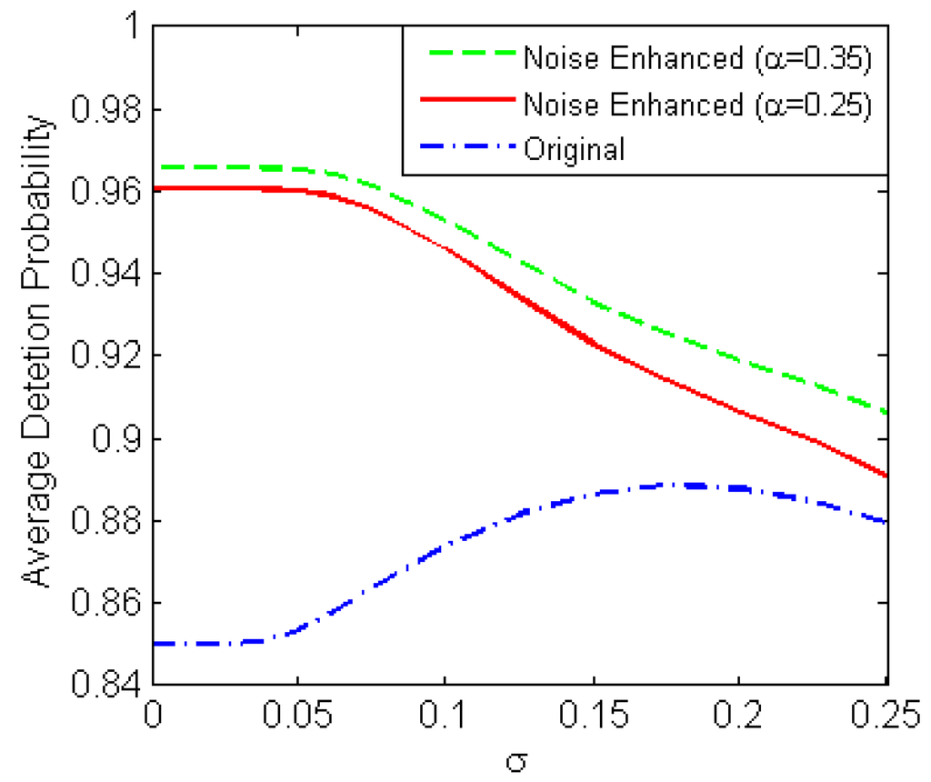
Figure 3.
Average detection probabilities versus obtained by the original detector and the noise-enhanced restricted NP approach for and when , , and .
Figure 4 compares the maximum noise-enhanced average detection probabilities and the corresponding minimum noise modified detection probabilities, which are obtained by the restricted NP approach for and 0.7, classical NP, Max–min approaches, and the original detector, versus when , , and . It should be noted that the average detection probability is equal to the minimum detection probability for the noise-enhanced Max–min approach and the original detector. As shown in Figure 4, the noise-enhanced classical NP approach produces the highest average detection probability and the lowest minimum detection probability, while the noise-enhanced Max–min approach obtains the maximum of the minimum detection probability. The results are consistent with the analysis in Section 3.3.
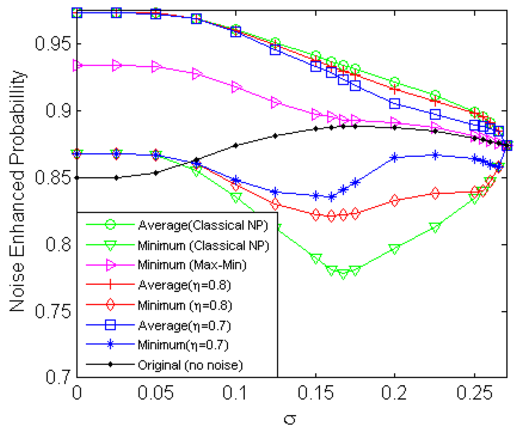
Figure 4.
Average and minimum detection probabilities versus obtained by the original detector and the noise-enhanced restricted NP (for and ), classical NP, and Max–min approaches when, , and .
When is close to 0, the average detection probability and the corresponding minimum detection probability obtained by the noise-enhanced restricted NP approach are the same as those obtained by the noise-enhanced classical NP approach, and the minimum detection probability is still greater than the original detection probability. In addition, the change of has little or no effect on the optimal additive noise in this case. With the increase of , the average detection probabilities obtained in the three noise-enhanced approaches decrease gradually; the corresponding minimum probabilities first decrease and then increase slightly. The minimum detection probability obtained by the noise-enhanced Max–min approach decreases and gradually approaches the original detection probability. Furthermore, for a certain range of , a greater average detection probability and a smaller minimum detection probability are obtained by the noise-enhanced restricted NP approach for a greater value of . In addition, no improvement of the detectability can be achieved by adding any noise when exceeds a certain level.
5. Conclusions
In this paper, the noise-enhanced signal detection for the composite hypothesis problem is studied according to various criteria. The noise-enhanced detection problem is formulated as a noise-enhanced classical Neyman–Pearson (NP), Max–min, or restricted NP problem when the prior information is completely known, completely unknown, or partially known, respectively. The relationships of the noise-enhanced restricted NP problem, classical NP problem, and Max–min problem are discussed. Further, the optimal additive noise obtained according to the restricted NP criterion was analyzed from a special perspective where the noise-enhanced restricted NP problem is equivalent to a noise-enhanced classical NP problem with different prior distributions under certain conditions, and the related algorithm is provided to find the optimal solution. The minimum detection probability corresponding to the maximum noise-modified average detection probability is proven to equal , which is the lower limit of detection probability in the restricted NP framework. In addition, it is demonstrated that the maximum noise-modified average detection probability obtained by the restricted NP approach is a strictly decreasing and concave function of . Finally, numerical examples and simulation results are provided to illustrate and verify the theoretical analysis.
In conclusion, the detection performance can be improved by adding additive noise obtained by the restricted NP, classical NP, and Max–min approaches. Specifically, a better Receiver Operating Characteristic (ROC) can be obtained. Under certain conditions, a better ROC means an increase of SNR. Therefore, we could consider extending the theoretical results in this paper to increase the SNR in the quantum regime, or to explore the optimal additive noise that enhances the quantum resonance [3,4,5,6,7]. For example, a superconducting quantum interference device (SQUID) is usually used to convert an applied magnetic flux into a voltage signal [5,6,7]. First, we may treat the applied magnetic flux as the system input, and then obtain different output voltages via the addition of different direct current (DC) signals to the input. Thus, the corresponding noise-modified SNRs could be calculated. If there is no constraint on the input and/or output, the optimal additive noise would be the DC signal corresponding to the maximum noise-modified SNR.
Acknowledgments
This research is partly supported by the Basic and Advanced Research Project in Chongqing (Grant No. cstc2016jcyjA0134, No. cstc2016jcyjA0043) and the National Natural Science Foundation of China (Grant No. 61501072, No. 61471073, No. 41404027, and No. 61301224).
Author Contributions
Shujun Liu raised the idea of the new framework to solve different noise-enhanced composite hypothesis-testing problems under different criteria. Ting Yang and Shujun Liu contributed to the drafting of the manuscript, interpretation of the results, some experimental design, and checked the manuscript. Mingchun Tang and Hongqing Liu designed the experiment of maximum noise-modified average detection probabilities obtained by the restricted NP approach. Kui Zhang and Xinzheng Zhang contributed to the proofs of the theories developed in this paper. All authors have read and approved the final manuscript.
Conflicts of Interest
The authors declare no conflict of interest.
Appendix A
Theorem A1.
Define a PDF of under as , where is any valid PDF. If there exists a PDF such that
where is the optimal additive noise PDF to maximize the average detection probability based on under the constraint that , then is the optimal solution of Equations (18) and (19).
Proof.
where the first inequality holds because , and the equality holds if and only if .
Since is the optimal additive noise PDF corresponding to the maximum average detection probability based on and under the constraint that , we have
If , we have
In conclusion, is the solution of Equations (18) and (19). In addition, Equation (18) is always less than or equal to (A4). □
Corollary A1.
Under the conditions in Theorem 1, if , is the optimal additive noise PDF corresponding to the optimization problem described in Equations (10) and (11).
Proof.
From the definition of in Theorem 1, achieves the maximum of Equation (18), and the following inequality always holds under the constraint that . That is
Since according to Equation (11) and as assumed in the corollary, should be less than or equal to in order to make the inequality in (A5) true. Therefore, when under the conditions in Theorem 1, is the solution of Equations (10) and (11). □
Theorem A2.
Under the conditions in Theorem 1, is the PDF that minimizes the noise-modified average detection probability among all probability distributions of the form , where , and is any PDF. In other words, the following inequality holds:
where and are the optimal additive noise PDFs obtained by the classical NP approach corresponding to and , respectively.
Proof.
Under the conditions in Theorem 1, we have
Since , for any , one obtains
The last inequality holds due to the definition of . From Equation (A8), the maximum noise-modified average detection probability corresponding to is less than or equal to that corresponding to for . □
Theorem A3.
When , the maximum noise-modified detection probability obtained by the restricted NP approach is a strictly decreasing and concave function of .
Proof.
First, based on the definition of the noise-enhanced restricted NP approach, is a non-increasing function of . In order to prove the concavity of with respect to (w.r.t.) , we define an additive noise with PDF , which is a convex combination of two optimal additive noises obtained by the restricted NP approach under the same constraint on false-alarm probability corresponding to and . That is,
where , , , and denote the optimal additive noise PDFs obtained by the restricted NP approach for and , respectively. From the definition of , the noise-modified detection and false-alarm probabilities corresponding to for a given value of can be obtained as
From the relation in Equation (A11), it is obvious that also satisfies the constraint on false-alarm probability. That is,
Based on Equations (A9) and (A10), the noise-modified average detection probability corresponding to can be calculated by
Accordingly, the minimum detection probability obtained by adding the noise with PDF can be upper bounded by
Let and , the following inequalities can be obtained according to Equations (A13) and (A14),
where the first inequality holds due to the non-increasing character of w.r.t. and the second inequality follows because is the optimal additive noise to maximize the noise-modified average detection probability for the case where the constraint on the minimum detection probability is selected as . Therefore, is proven to be a concave function w.r.t. .
Next, the strictly decreasing character of will be shown. Let and suppose , which means is also an optimal additive noise corresponding to . We then have , which obviously contradicts Equation (31). Therefore, must satisfy for any .
In summary, is a strictly decreasing concave function w.r.t. . □
References
- Benzi, R.; Sutera, A.; Vulpiani, A. The mechanism of stochastic resonance. J. Phys. A Math. Gen. 1981, 14, 453–457. [Google Scholar] [CrossRef]
- Löfstedt, R.; Coppersmith, S.N. Quantum stochastic resonance. Phys. Rev. Lett. 1994, 72, 1947–1950. [Google Scholar] [CrossRef] [PubMed]
- Grifoni, M.; Hänggi, P. Nonlinear quantum stochastic resonance. Phys. Rev. E 1996, 54, 1390–1401. [Google Scholar] [CrossRef]
- Hibbs, A.D.; Singsaas, A.L. Stochastic resonance in a superconducting loop with a Josephson junction. J. Appl. Phys. 1995, 77, 2582–2590. [Google Scholar] [CrossRef]
- Rouse, R.; Han, S.; Lukens, J.E. Flux amplification using stochastic superconducting quantum interference devices. Appl. Phys. Lett. 1995, 66, 108–110. [Google Scholar] [CrossRef]
- Glukhov, A.M.; Sivakov, A.G. Observation of stochastic resonance in percolative Josephson media. Low Temp. Phys. 2002, 28, 383–386. [Google Scholar] [CrossRef]
- Patel, A.; Kosko, B. Stochastic resonance in continuous and spiking neuron models with Levy noise. IEEE Trans. Neural Netw. 2008, 19, 1993–2008. [Google Scholar] [CrossRef] [PubMed]
- Addesso, P.; Filatrella, G.; Pierro, V. Characterization of escape times of Josephson junctions for signal detection. Phys. Rev. E 2012, 85, 016708. [Google Scholar] [CrossRef] [PubMed]
- Weber, J.F.; Waldman, S.D. Stochastic Resonance is a Method to Improve the Biosynthetic Response of Chondrocytes to Mechanical Stimulation. J. Orthop. Res. 2015, 34, 231–239. [Google Scholar] [CrossRef] [PubMed]
- Zozor, S.; Ambland, P.O. On the use of stochastic resonance in sine detection. IEEE Process. 2002, 7, 353–367. [Google Scholar] [CrossRef]
- Zozor, S.; Ambland, P.O. Stochastic resonance in locally optimal detectors. IEEE Process. 2002, 51, 3177–3181. [Google Scholar] [CrossRef]
- Patel, A.; Kosko, B. Noise benefits in quantizer-array correlation detection and watermark decoding. IEEE Trans. Signal Process. 2011, 59, 488–505. [Google Scholar] [CrossRef]
- Chen, H.; Varshney, L.R.; Varshney, P.K. Noise-enhanced information systems. Proc. IEEE 2014, 102, 1607–1621. [Google Scholar] [CrossRef]
- Han, D.; Li, P.; An, S.; Shi, P. Multi-frequency weak signal detection based on wavelet transform and parameter compensation band-pass multi-stable stochastic resonance. Mech. Syst. Signal Process. 2016, 70, 995–1010. [Google Scholar] [CrossRef]
- Addesso, P.; Pierro, V.; Filatrella, G. Interplay between detection strategies and stochastic resonance properties. Commun. Nonlinear Sci. Numer. Simul. 2016, 30, 15–31. [Google Scholar] [CrossRef]
- Stocks, N.G. Suprathreshold stochastic resonance in multilevel threshold systems. Phys. Rev. Lett. 2000, 84, 2310–2313. [Google Scholar] [CrossRef] [PubMed]
- Kosko, B.; Mitaim, S. Stochastic resonance in noisy threshold neurons. Neural Netw. 2003, 16, 755–761. [Google Scholar] [CrossRef]
- Kosko, B.; Mitaim, S. Robust stochastic resonance for simple threshold neurons. Phys. Rev. E 2004, 70, 031911. [Google Scholar] [CrossRef] [PubMed]
- Mitaim, S.; Kosko, B. Adaptive stochastic resonance in noisy neurons based on mutual information. IEEE Trans. Neural Netw. 2004, 15, 1526–1540. [Google Scholar] [CrossRef] [PubMed]
- Gingl, Z.; Makra, P.; Vajtai, R. High signal-to-noise ratio gain by stochastic resonance in a double well. Fluct. Noise Lett. 2001, 1, L181–L188. [Google Scholar] [CrossRef]
- Makra, P.; Gingl, Z. Signal-to-noise ratio gain in non-dynamical and dynamical bistable stochastic resonators. Fluct. Noise Lett. 2002, 2, L145–L153. [Google Scholar] [CrossRef]
- Makra, P.; Gingl, Z.; Fulei, T. Signal-to-noise ratio gain in stochastic resonators driven by coloured noises. Phys. Lett. A 2003, 317, 228–232. [Google Scholar] [CrossRef]
- Kay, S. Can detectability be improved by adding noise? IEEE Signal Process. Lett. 2000, 7, 8–10. [Google Scholar] [CrossRef]
- Chen, H.; Varshney, P.K.; Kay, S.M.; Michels, J.H. Theory of the stochastic resonance effect in signal detection: Part I—Fixed detectors. IEEE Trans. Signal Process. 2007, 55, 3172–3184. [Google Scholar] [CrossRef]
- Chen, H.; Varshney, P.K.; Kay, S.M.; Michels, J.H. Theory of the stochastic resonance effect in signal detection: Part II—Variable detectors. IEEE Trans. Signal Process. 2007, 56, 5031–5041. [Google Scholar] [CrossRef]
- Patel, A.; Kosko, B. Optimal noise benefits in Neyman–Pearson and inequality constrained signal detection. IEEE Trans. Signal Process. 2009, 57, 1655–1669. [Google Scholar] [CrossRef]
- Bayram, S.; Gezici, S. On the Restricted Neyman–Pearson Approach for composite hypothesis-testing in presence of prior distribution uncertainty. IEEE Trans. Signal Process. 2011, 59, 5056–5065. [Google Scholar] [CrossRef]
- Bayram, S.; Gezici, S. Stochastic resonance in binary composite hypothesis-testing problems in the Neyman–Pearson framework. Digit. Signal Process. 2012, 22, 391–406. [Google Scholar] [CrossRef]
- Bayram, S.; Gultekin, S.; Gezici, S. Noise enhanced hypothesis-testing according to restricted Neyman–Pearson criterion. Digit. Signal Process. 2014, 25, 17–27. [Google Scholar] [CrossRef]
- Bayram, S.; Gezici, S. Noise-enhanced M-ary hypothesis-testing in the mini-max framework. In Proceedings of the 3rd International Conference on Signal Processing and Communication Systems, Omaha, NE, USA, 28–30 September 2009; pp. 1–6.
- Bayram, S.; Gezici, S.; Poor, H.V. Noise enhanced hypothesis-testing in the restricted bayesian framework. IEEE Trans. Signal Process. 2010, 58, 3972–3989. [Google Scholar] [CrossRef]
- Bayram, S.; Gezici, S. Noise enhanced M-ary composite hypothesis-testing in the presence of partial prior information. IEEE Trans. Signal Process. 2011, 59, 1292–1297. [Google Scholar] [CrossRef]
- Kay, S.M.; Michels, J.H.; Chen, H.; Varshney, P.K. Reducing probability of decision error using stochastic resonance. IEEE Signal Process. Lett. 2006, 13, 695–698. [Google Scholar] [CrossRef]
- Lehmann, E.L. Testing Statistical Hypotheses, 2nd ed.; Chapman & Hall: New York, NY, USA, 1986. [Google Scholar]
- Richards, M.A. Fundamentals of Radar Signal Processing; McGraw-Hill Profrssional Engineering: New York, NY, USA, 2005. [Google Scholar]
- Zarrin, S.; Lim, T.J. Composite hypothesis testing for cooperative spectrum sensing in cognitive radio. In Proceedings of the IEEE International Conference on Communications, Dresden, Germany, 14–18 June 2009; pp. 1721–1725.
- Hodges, J.L., Jr.; Lehmann, E.L. The use of previous experience in reaching statistical decisions. Ann. Math. Stat. 1952, 23, 396–407. [Google Scholar] [CrossRef]
© 2016 by the authors; licensee MDPI, Basel, Switzerland. This article is an open access article distributed under the terms and conditions of the Creative Commons Attribution (CC-BY) license (http://creativecommons.org/licenses/by/4.0/).