Self-Organization with Constraints—A Mathematical Model for Functional Differentiation

Abstract

This study proposes mathematical models for functional differentiations that are viewed as self-organization with external constraints. From the viewpoint of system development, the present study investigates how system components emerge under the presence of constraints that act on a whole system. Cell differentiation in embryos and functional differentiation in cortical modules are typical examples of this phenomenon. In this paper, as case studies, we deal with three mathematical models that yielded components via such global constraints: the genesis of neuronal elements, the genesis of functional modules, and the genesis of neuronal interactions. The overall development of a system may follow a certain variational principle.

1. Introduction

In this study, we propose a theory for the differentiation of system components (i.e., elements) caused by a constraint that acts on a whole system. We describe three mathematical models for functional differentiation in the brain; the first model for the genesis of neuron-like excitable components, the second for the genesis of cortical modules, and the third for the genesis of neuronal interactions, thereby emphasizing the importance of constrained dynamics of self-organization.

First, let us briefly review the conventional theory of self-organization. Here, we will omit the long-term discussions regarding the significance of self-organization that occurred in the fields of philosophy and social sciences. We will describe only the phenomena and theories of self-organization in the areas of natural science and engineering. As far as we know, such studies of self-organization started, in association with the movement of cybernetics that took place between 1940 and 1950, in which the theory of self-organization developed in the construction of control theory [1]. For example, Ashby proposed the principle of the self-organizing dynamic system [2], in which a dynamic system is a different concept from an (autonomous) dynamical system, in the sense that the former includes input, whereas the latter has no input, in particular, situations of input changes are treated only as bifurcations in a family of dynamical systems. He stated that the asymptotic state of any deterministic dynamic system is an attractor, where each subsystem interacts with other subsystems that play a role in the environment of such a subsystem, thus forming a controlled overall system. Von Foerster proposed the principle of order out of noise, emphasizing the importance of random fluctuations for producing a macroscopic-ordered and controlled motion [3].

From the 1960s to the 1980s, the appearance of two scientific leaders in physics and chemistry, i.e., Haken and Prigogine led to the scientific revolution of self-organization in far-from-equilibrium systems. Those scientists faced the challenge of constructing theories for nonequilibrium statistical physics and nonequilibrium thermodynamics, respectively, in which “nonequilibrium” meant “far from equilibrium”. In fact, Prigogine extended thermodynamics to the area of nonlinear and far-from-equilibrium systems in terms of the variational principle of entropy production minimum [4]. Because energy dissipation is a prerequisite in far-from-equilibrium systems, the concept of entropy flow associated with energy dissipation should be introduced. In this respect, the entropy production σ is defined as the sum of the change in the internal entropy of the system in question and the outflow of the entropy from the system to the environment, as follows:

$$\sigma = \frac{d{S}_{int}}{dt}+ J_{S_{out}}$$

(1)

Another significant approach was taken by Haken regarding the extension of equilibrium phase transitions to far-from-equilibrium systems, thus introducing the slaving principle [5]. In fact, Haken extended the Ginzburg–Landau (GL) formula to far-from-equilibrium and multicomponent systems; the original GL equation is given in the form of the equation of motion of order parameter D (see [5] for more details):

$$\frac{\partial D}{\partial t}= \alpha D- \frac{W}{2} |D{|}^{2}D$$

(2)

Many modes appear in each bifurcation point, which corresponds to the critical point of phase transition; however, a few modes enslave the many other modes, which implies the appearance of order parameters out of fluctuations. Therefore, the slaving principle extends the center manifold theorem in bifurcation theory to systems with noise [6]. However, the slaving principle does not hold in the appearance of chaos; thus, it is applicable to the index of chaotic motion.

The occurrence of macroscopic-ordered motion via cooperative and/or competitive interactions between the microscopic components of the system, namely atomic or molecular level interactions, is a characteristic of the self-organizing phenomena that are addressed by these theories. In other words, the theories mentioned above treat the manner via which spatiotemporal patterns emerge as macroscopic-ordered states from microscopic random motion under far-from-equilibrium conditions. They succeeded in describing the phenomena, for example, of target patterns, spiral patterns, propagating waves, periodic and chaotic oscillations in chemical reaction systems (such as the Belousov–Zhabotinsky system), hydrodynamic systems (such as the Bénard thermal convection system and the Taylor–Quette flow system), and optical systems (such as the laser oscillations system).

Another aspect may be highlighted when considering typical communication problems, as the brain activity in each communicating person may change according to the purpose of the communication (see, for example, [7,8,9,10]). It seems that this aspect can be formulated within a framework of functional differentiation in which the functional elements (or components, or subsystems) are produced by a certain constraint that acts on the whole system [11,12,13]. In fact, the functional differentiation of the brain occurs via not only genetic factors, but also dynamic interactions between the brain and the environments [14,15,16,17]. Pattee [18] discriminates constraints from dynamics. He stated that dynamics occurs via interactions of elements of the systems and also via external forces, whereas a constraint is given intentionally by the outside of the system, thereby controlling the system dynamics. Furthermore, he introduced a conceptual test to discriminate dynamics from constraints in terms of the rate dependence and the rate independence, respectively. In this respect, here, we use the term, constraints in a sense that is similar to that of Pattee. In neonatal and successive periods of development, an individual brain experiences structural and functional differentiation, which can be promoted by environmental factors such as the intentions and actions of surrounding people, as well as physical stimuli, such as object patterns. These intentions and actions, which convey a part of the environmental meaning, can become constraints of self-organization of neural dynamics in individual brains. Conversely, physical stimuli can be treated as time-dependent inputs (see, Equation (3)).

Based on these ideas of constraints, we will introduce constraints, by which the system dynamics is optimized. Let $(\varphi , \mathsf{\Omega }$) be a dynamical system, where $\mathsf{\Omega }$ is a m-dimensional state space or phase space and$\varphi$ is a flow or a group action acting on the space $\mathsf{\Omega }$. Let $x$ be a state variable defined in $\mathsf{\Omega }$. Then, a dynamical system can be represented by the equations of motion: $\frac{dx}{dt}=f\left(x\right),$ where t is a parameter defined outside the space $\mathsf{\Omega }$, which is usually interpreted as time, and f is a dynamical law or a vector field. A dynamical system may possess other parameters called bifurcation parameters, which can be controlled from outside, and those bifurcation parameters indicate environmental conditions, which should be viewed as being different from constraints [19]. Then, the equations are rewritten as $\frac{dx}{dt}=f\left(x;\lambda \right),$ including the bifurcation parameters, thus representing a family of dynamical systems. However, the system that we wish to consider here should include environmental variables, which may have a feedback from the system variables, thus expressed as $G(x,t)$. The feedback may happen via system order parameters (see, for example, [19]), or constraints. A possible formulation is given by Equations (3) and (4).

$$\frac{dx}{dt}=f\left(x, \lambda \right)+G\left(x, t\right)$$

(3)

under the given constraint, $\complement$, which denotes the intention of the outside. In particular, here we consider the restricted cases of the constraint to integrable functions, such as certain information quantities, which are supposed to be derived from intention. If this supposition is allowed, an overall formula can be provided by the variational principle:

$$\mathsf{\delta }L=\mathsf{\delta }\underset{0}{\overset{T}{\int }}\{\complement + \mu (\frac{dx}{dt}-f\left(x, \lambda \right)-G\left(x, t\right))\}dt=0$$

(4)

where $\mu$ is a Lagrange multiplier. In usual mechanics with a physical constraint such as the movement of a ball on a playground slide, a Lagrange multiplier is introduced to allow a particle to move along such a boundary. However, in the case of optimal control problems, a Lagrange multiplier can be introduced to satisfy a dynamical system with external inputs, and variations can be adopted to optimize the external constraint $\complement$ under the restriction of the dynamics given by Equation (3) [20,21]. Thus, a Lagrange multiplier may be a function not only of a state variable x, but also of its rate $\dot{x}$ and time t, and equations of motion of such a multiplier may be derived. In the present paper, we use the maximum transmission of information as a constraint. In relation to the present approach, in the recent development of a synergetic computer, Haken and Portugali [22] introduced the notion of information adaptation to realize pattern recognition based on pattern formation in synergetic networks using attention parameters as a constraint.

It should be noted that in the self-organization process, in addition to the constrained dynamics in the sense mentioned above, various types of synaptic learning may take place, such as Hebbian learning and winner-take-all algorithms. These learning algorithms may provide internal constraints to the dynamics. This type of internal constraints is supposed to be contained in the dynamics given by Equation (3). A typical internal constraint to the neural dynamics was intensively investigated by von der Malsburg in studies of self-organization of orientation-sensitive cells in the primary visual cortex [23]. In the model, decisive effects on the neural differentiation of orientation specificity may be provided by a synaptic constraint: for each neuron the total strength of synaptic couplings is kept constant, the internal constraint of which may be reasonable when considering the case of almost the same quantity of nutrition supplied to each neuron in a spatially uniform circumstance. Furthermore, Kohonen invented the self-organizing map (SOM), with at least two different subsystems: one is a competitive neural network with a winner-take-all algorithm and the other called a plasticity-control subsystem, which produces feature-specific differentiation of input data [24]. Amari also developed a mathematical model for topographic mapping by introducing a generalized Hebb synapse, a plasticity of inhibitory interneurons as well as excitatory neurons and competitive neural networks by mutual inhibition [25]. Thus, competitive neural networks impose a local constraint on the activity of elementary neurons, thereby enhancing the feature differences of input data, which gives rise to differentiation. In addition to the neural systems, a similar differentiation triggered by internal constraints has been observed in bacterial populations and was simulated by its theoretical models [26,27]. In these studies, Kaneko and Yomo, and Furusawa and Kaneko, found that fluctuations are enhanced to realize cell differentiation by cell divisions, which are triggered by an internal constraint, such as keeping the total nutrition in each cell constant.

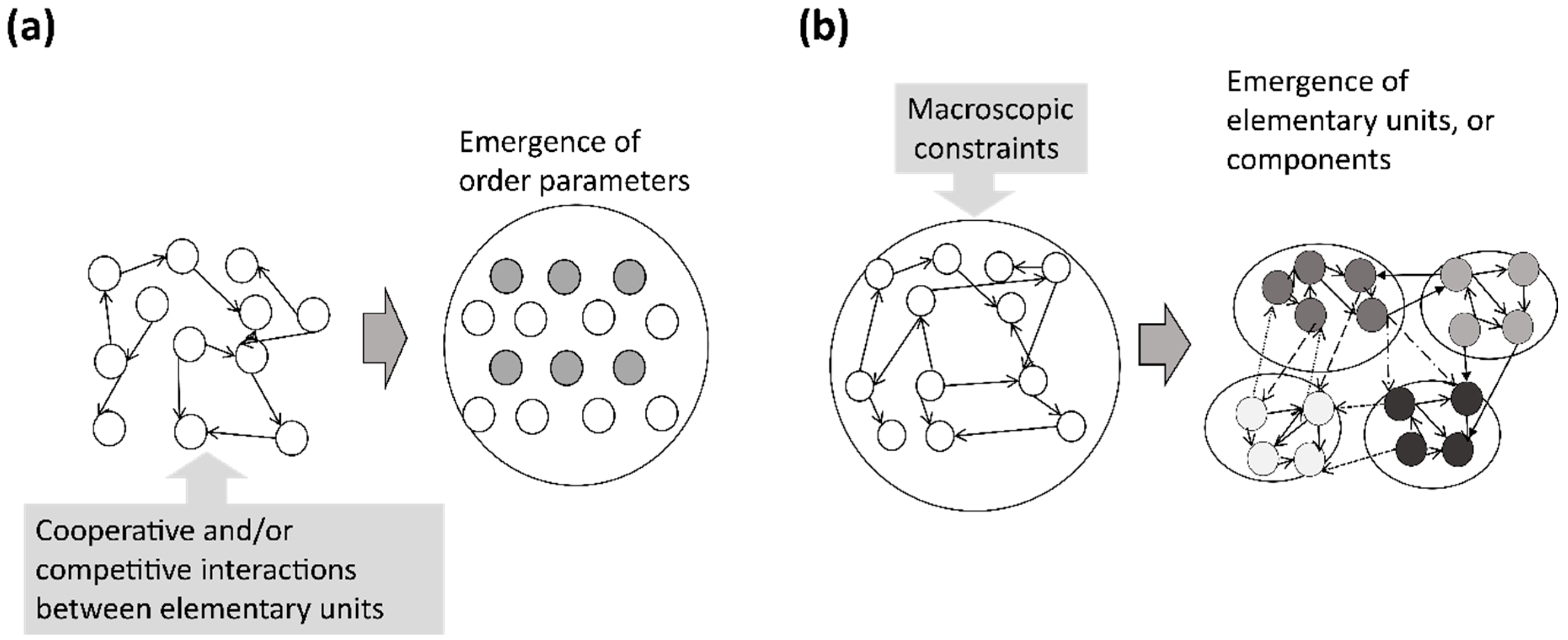
Based on these aspects, different features of self-organization from a typical macroscopic pattern formation formulated by, for instance, coupled dynamical systems and reaction-diffusion systems may exist (see Figure 1). In this paper, we propose mathematical models that show the differentiation of system components from a constraint acting on a whole system, i.e., at the macroscopic level. In our model study, a genetic algorithm was used for the computation of the development of both the interactions and the states of the dynamical systems. In this computational process, a maximum transmission of information constraint was applied as a “variational” principle to operate the development of the system. In the subsequent sections, we will show the computational results of our mathematical models for neural differentiation, and will review (with some comments) a mathematical formula for ephaptic couplings, which may provide a possible neural mechanism of self-consistent dynamics with constraints.

2. Mathematical Model for the Differentiation of Neurons

To elucidate the neural mechanism underlying the genesis of neurons, we have tried to generate a mathematical model of the differentiation of neurons in terms of the development of dynamical systems under a constraint [28,29]. As a case study, we used the one-dimensional map given by Equation (5), which is viewed as an elementary unit of the system.

$$x\left(t+1\right)=\tanh \left({\gamma }_1\left(x\left(t\right)-{\alpha }_{1 }\right)\right)-\omega \tanh \left({\gamma }_2\left(x\left(t\right)-{\alpha }_2\right)\right)+J$$

(5)

where $x\in \left(-\infty ,\infty \right)$ is a state variable, t is a discrete time step, and the parameters ${\gamma }_i\left(i=1,2\right), {\alpha }_i\left(i=1,2\right), \omega ,$ and J are real numbers.

The total system computed here is constituted by the unidirectional nearest neighbor coupling of these units, but can be extended to include feedback couplings. We show in this paper only the computation results of the case of unidirectional couplings with an open boundary condition. Input time series are added to this system. Then the coupled system is described by Equation (6).

$$x^{(i)}(t+1)= \tanh ({\gamma }_1(x^{(i)}(t)-{\alpha }_{1 }))-\omega \tanh ({\gamma }_2(x^{(i)}(t)-{\alpha }_2))+d(x^{(i-1)}-x^{(i)})$$

(6)

where $x^{(i)}(t)$ denotes the state of the i-th unit at time t, d is the coupling strength (which was kept constant in each simulation).

We adopted a genetic algorithm for these networks, with an external input. We used a chaotic time series as the external input. Because bifurcation parameters of dynamical systems are provided as environmental variables that are kept constant during the state changes of dynamical systems, a set of these parameters $({\gamma }_{1, }{\gamma }_{2, }{\alpha }_{1, }{\alpha }_{2, }\omega , J)$ is viewed as a “gene” of the dynamical system in question. In this model, as an external constraint, we used the maximum transmission of information of input data to all units of the coupled system. In the present model, the external constraint $\complement$ in Equation (4) changes in time much slower than the system dynamics itself.

Then, for each network, we calculated the time-dependent mutual information [30] between the input chaotic time series and the time series of each structural unit of the network. The time-dependent mutual information between input time series $g\left(t\right)$ and i-th unit is defined in the following way.

$$I(g\left(t\right);x^{\left(i\right)}(t))(t)=-{\sum }_{k}p\left(k\right)\log p\left(k\right)+ {\sum }_{l, k}p(l)p^{(t)}(k/l)\log p^{(t)} (k/l)$$

(7)

where k denotes a state of $x^{\left(i\right)}(t)$ and p(k) represents a stationary probability of $x^{\left(i\right)}(t)$, l denotes a state of the input time series $g\left(t\right)$, and $p^{(t)}(k/l)$ is a conditional probability of $x^{\left(i\right)}(t)$ taking a state k at t time steps after $g\left(t\right)$ taking a state l. In general, mutual information between two states calculates the information shared between these states. Thus mutual information does not necessarily imply the transmitted information. However, in the unidirectionally coupled system with inputs, such as the present system, shared information calculated by mutual information includes mainly the information transmitted from one to the other.

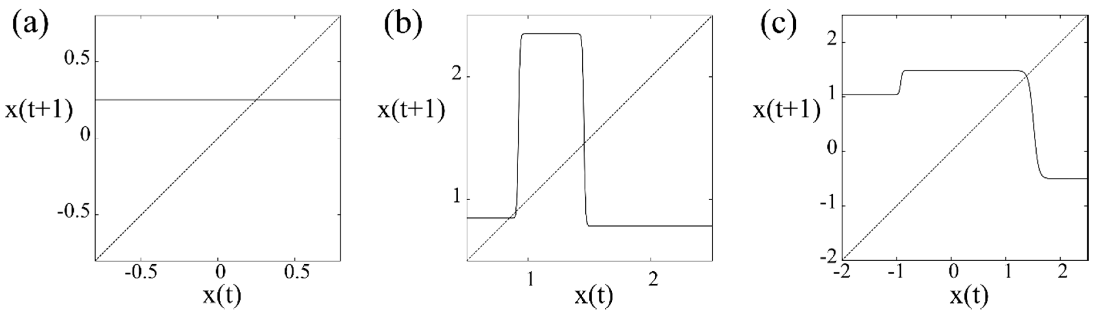
Then, we recorded its maximum value over time, and a maximum value over units. Subsequently, in the genetic algorithm, we adopted a copy, crossover, and mutations for the above-mentioned set of parameters $\left({\gamma }_{1, }{\gamma }_{2, }{\alpha }_{1, }{\alpha }_{2, }\omega , J\right)$, and followed by the selection of a dynamical system that allowed more information transmission compared with the previous step of the development. The coupling strength was fixed over all simulations. However, depending on the coupling strength, the computational results were classified as three types of information channels in the following way.

(a) The case of strong couplings

A dynamical system that was constructed using a constant function was finally selected (see Figure 2a). This type of dynamical system possesses a single stable fixed point. Any external signals were successfully transmitted over all elementary units of the network without any deformation. Thus, this type of network can be viewed as a static channel.

(b) The case of intermediate strength couplings

An excitable dynamical system that was constructed using a step function was finally selected (see Figure 2b). This type of dynamical system possesses three fixed points: one is stable and the other two are unstable. One of the unstable fixed points plays a role as a threshold in the sense that if the initial condition is set below the threshold, a dynamical trajectory is monotonously attracted to the stable fixed point; otherwise, it is attracted to this point only after a dynamical trajectory experiences a large excursion around another unstable fixed point. Thus, the stable fixed point can be viewed as an equilibrium membrane potential, and the large excursion of the dynamical trajectory can also be viewed as a transient impulse. Furthermore, the latter type of dynamical trajectory can overshoot the stable fixed point after a large excursion, and is then attracted to the fixed point. Therefore, this excitable dynamical system can be viewed as an active channel, such as those observed in conventional neurons.

(c) The case of weak couplings

An oscillatory dynamical system was finally selected (see Figure 2c). In the present model, this type of dynamical system possessed a period two periodic trajectory. Thus, it can be viewed as an oscillatory neuron.

The evolution model treated here was restricted to a certain subspace of functional space, which spanned only a restricted functional space, even compared with polynomials. However, it seems to be reasonable to propose the present model as showing rather universal characteristics, despite this restriction. One explanation for this observation is that eventually evolved dynamical systems are optimal to produce weak chaotic behaviors in the overall dynamics of coupled systems, such as allowing effective information transmission, regardless of coupling strength. The other explanation is that dynamical systems constructed using polynomial functions cannot survive under the present constraint as their coupled systems cannot transmit information of dynamically changing input because of the extremely narrow parameter range that allows an effective transmission of input information. One can extend the present model further to develop the dynamics in wider functional subspace; however, this is associated with several technical problems, such that it is not easy to define automatically the domain of definition that is necessary to restrict the overall dynamics in a certain finite domain.

In the present model, which was constructed using a coupled one-dimensional map, the elementary unit of the overall system was a one-dimensional map. The present simulations showed an evolution dynamics in which the dynamical law in each elementary unit was changed according to the external constraint, such as the maximum transmission of the input information. The dynamical system finally selected was an excitable map or oscillatory map, with the exception of a trivial case. The simulation results may provide an explanation for the generation of excitable or oscillatory systems, such as neurons in biological evolution.

3. Mathematical Model for the Differentiation of Cortical Modules

In this section, we describe a mathematical model that produced distinct modules from probabilistically uniform modules because of the symmetry breaking caused by the appearance of chaotic behaviors. In the proposed mathematical model, a phase model of oscillators was used as an elementary unit of the system; however, we show that these elementary units do not necessarily evolve as functional units. This study aimed at elucidating the neural mechanism underlying the functional differentiation of cortical areas which are known as Brodmann’s areas [31], and consists of about 10,000 functional modules [32,33]. It is well known that the mammalian neocortex consists of almost uniform modules, each of which contains about 5,000 excitatory pyramidal neurons and several kinds of inhibitory neurons. In spite of this uniformity, cortical modules have distinct functions; hence, it is highly probable that functional differentiation is caused by the presence of asymmetric couplings between modules. Such cortical asymmetric couplings possess the following generic characteristics: ascending couplings project from superficial layers, such as layers I–III, to a middle layer, such as layer IV, whereas descending couplings project from deep layers, such as layers V and VI, to both superficial and deep layers [34].

To observe the process described above, we constructed a mathematical model for the structural differentiation of two modules, consisting of a number of units that is assumed to be uniform in a probabilistic sense [35]. In fact, before the development of the modules, the coupling probabilities between units within each module and between modules were determined randomly, so that the system was viewed as simply one module at the beginning of the development. For the sake of brevity, we formally divided the system into two probabilistically identical modules and observed the formation of feature differences of couplings between elementary units. We adopted a Weyle transformation as a unit, and the couplings were provided by the sinusoidal function, which is similar to a discrete time version of the Kuramoto model [36], as follows:

$${\theta }_{t+1}^{(i,k)}={\omega }^{(i,k)}+{\theta }_t^{(i,k)}+\frac{\alpha }{N{p}^c}{\displaystyle \sum }_{(j,l)\in G^{(i,k)}}\sin \left({\theta }_t^{(j,l)}-{\theta }_t^{\left(i,k\right)}-{\psi }_{kl}^{ij}\right)+{\sigma }_{\beta }{\beta }_t^{(i,k)}$$

(8)

for the k-th unit in the ith modules. Here, $\psi$ is assigned one of four possible values $\left\{0,\frac{\pi }{2},\pi ,\frac{3\pi }{2}\right\}$ randomly, according to the probabilities, and $\beta$ denotes Gaussian noise and ${\sigma }_{\beta }$ is the strength of the Gaussian noise. Moreover, $\alpha$ is the coupling strength of units, N is the total number of units, and $p_c$ is the overall coupling probability of units, i.e., the ratio of coupled units to the total number of units. In this model, as an external constraint, we used the maximum transmission of information. In the present model, the external constraint $\complement$ in Equation (4) changes in time much slower than the system dynamics itself.

Then, by changing these probabilities, the product of transfer entropies defined by Equations (9) and (10) was calculated, and the system with the maximum product of transfer entropies was selected at each stage of the development.

$$T\equiv T_{{\mathsf{\Theta }}^{\left(1\right)}\to {\mathsf{\Theta }}^{\left(2\right)}}\cdot T_{{\mathsf{\Theta }}^{\left(2\right)}\to {\mathsf{\Theta }}^{\left(1\right)}}$$

(9)

$$T_{X\to Y}\left(\tau \right)=H\left(Y\left(t+\tau \right)|Y\left(t\right)\right)-H\left(Y\left(t+\tau \right)|Y\left(t\right),X(t)\right)$$

(10)

where H(A|B) denotes the conditional entropy of A under the condition of B.

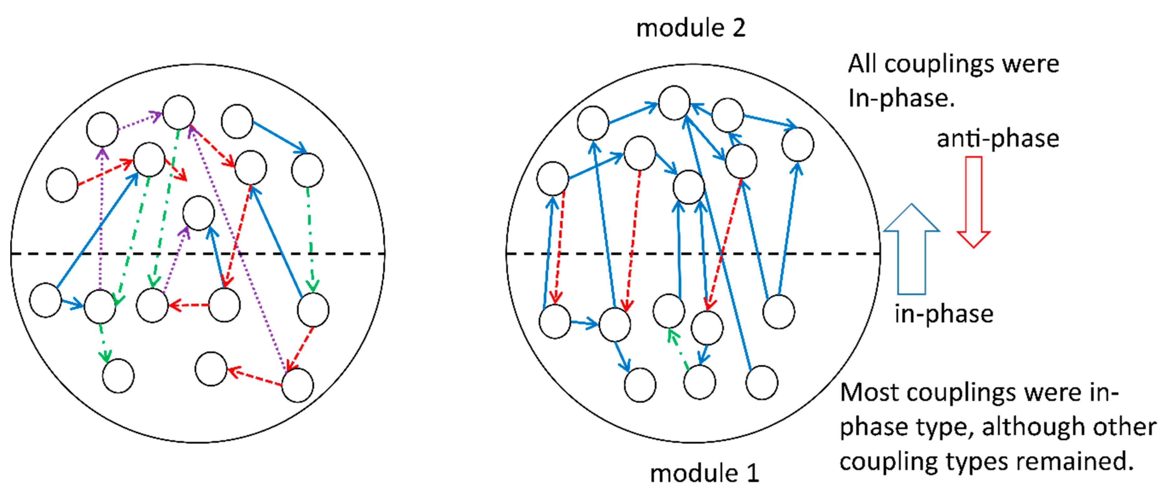
During the development of the system, we fixed the overall coupling probability of units, the number of units, and the additive Gaussian noise, whereas other coupling probabilities and probabilities for the phase shift, $\psi$, in the coupling terms were subjects for change. A set of these changeable parameters was viewed as a gene in the genetic algorithm. Subsequently, we observed the differentiation of the physical properties of modules, as follows. In one module, say module 1, most couplings were in phase, although other coupling types remained; in contrast, in the other module, say module 2, all surviving couplings were in phase. All the couplings from modules 1 to 2 were in phase, whereas the opposite direction of couplings was antiphase. The number of couplings from modules 1 to 2 was much larger than that observed for the opposite direction of couplings. The final form of differentiation is evolutionally stable in the sense that the system may evolve in a similar way and reach the same selected states as long as the present fixed values of parameters or varieties of fixed parameters are not changed. For example, the dynamics that were finally selected could change if some of the fixed parameters were changed after the evolution dynamics once became stable. Furthermore, it is expected that the number of elementary units in each module and the number of modules itself will change under the presence of input data. This problem will be the subject of future studies.

These computational results imply the appearance of a hierarchical structure of modules: module 1 governs module 2, i.e., module 1 for upper layers and module 2 for lower layers (see Figure 3). This implication comes from another observation in synergetics; that slaving modes behave cooperatively to form a few order parameters and slaved modes do not behave in such a way, showing more varieties of interactions [5,6]. Thus, the developed system may express a conscious mind for module 1 and a more unconscious mind (which might play a role in the direct interaction with the environment) for module 2. In other words, modules 1 and 2 may behave like higher and lower levels of functional units of the brain-body complex, respectively.

We also investigated the overall dynamics of the coupled module system. To observe the macroscopic dynamics, we defined two order parameters in the following way:

$$R^{(i)}(t)\exp (\sqrt{-1}{\Theta }^{(i)}(t))=\frac{1}{N}{\displaystyle \sum }_{k=1}^N\exp (\sqrt{-1}{\theta }_t^{(i,k)})$$

(11)

$$\Phi \left(t\right)={\Theta }^{(2)}\left(t\right)-{\Theta }^{(1)}\left(t\right)(\mathrm{mod}2\pi )$$

(12)

Here, phase coherence, $R^{\left(i\right)}\left(t\right)$ and mean phase, ${\Theta }^{\left(i\right)}\left(t\right)$, can be order parameters, although we used the relative mean phase defined by Equation (12) instead of a mean phase in each module. The dynamics observed via these order parameters showed weak “chaotic” behaviors, but included extremely slow oscillations, which covered periods of the order of a few seconds, compared with the time scale of around 200 ms of fundamental coherent oscillations. Similar slow oscillations of a period of a few seconds have been observed in the hippocampal CA1 of rats in several sleeping and running states [37]. Another similar interesting behavior has been observed in the dynamics of the default mode network, although such a time scale of modulation spanned around 20 min [38]. A typical functional differentiation via structural differentiation is observed in the hippocampus [39]: in reptiles, the hippocampus consists of unstructured, probabilistically uniform couplings of small and large neurons, whereas the hippocampus of mammals consists of mainly differentiated CA1 and CA3 areas. Compared with uniform couplings, the CA3 area possesses recurrent connections, whereas the CA1 area receives synaptic connections from the CA3 and sends its axons to other areas in the limbic systems and to the neocortex, rather than back to the CA3.

4. Redefined Neural Behaviors via Ephaptic Couplings: A Tractable System Governed by Self-Organization with Constraints

The two mathematical models described in Section 2 and Section 3 provide a possible neural mechanism by which components, or subsystems emerge via a constraint operating on a whole system. For the systems described above, only numerical studies have been conducted. The following mathematical model of ephaptic couplings between neurons represents an example of a similar system with more definite descriptions of the structure of the system in terms of the Fredholm condition. Moreover, a study of neural systems with ephaptic couplings reveals the importance of the role of neural fields in the formation of functional components that are not necessarily identified with the elementary units of self-organizing systems [40,41,42]. For example, a neuron can be an elementary unit in a neural system, but may not become a functional unit, as functional units may be formed in a structure with a larger size, e.g., in cell assemblies [42].

Markin provided a model for the ephaptic coupling between two identical neurons based on the equivalent electric circuit that presents such a physical coupling, as follows [43]:

$$\frac{r_2+r_3}{\gamma }\frac{{\partial }^2{V}_1}{\partial x^2} -c_1\frac{\partial V_1}{\partial t}=j_{ion1}+\frac{r_3}{\gamma }\frac{{\partial }^2{V}_2}{\partial x^2}$$

(13)

$$\frac{r_1+r_3}{\gamma }\frac{{\partial }^2{V}_2}{\partial x^2}-c_2\frac{\partial V_2}{\partial t}=j_{ion2}+\frac{r_3}{\gamma }\frac{{\partial }^2{V}_1}{\partial x^2}$$

(14)

where $V_1$ and $V_2$ denote the membrane potentials of two neurons, respectively; $r_1$ and $r_2$ are the resistivity of these neurons; $r_3$ is the ionic resistivity of the external medium; $\gamma =r_1{r}_2+r_2{r}_3+r_3{r}_1$; $c_1$ and $c_2$ are the capacitance; $j_{ion1}$, and $j_{ion2}$ are the ionic currents; and $t$ and $x$ denote time and space variables, respectively. Because the two neurons are assumed to be identical, we set $r_1=r_2$ and $c_1=c_2.$

In the following equations, we provide an essential part of the formulation, according to Scott [44]. The coupling constant can be expressed as $\alpha \equiv \frac{r_3}{r_1+r_3}=\frac{r_3}{r_2+r_3}$. Simple calculations of the coefficients in Equations (13) and (14) with $r_1=r_2$ lead the following equations: $\frac{r_1+r_3}{\gamma }=\frac{r_1+r_3}{\left\{r_1\left(r_1+r_3\right)+ r_1{r}_3\right\}}= \frac{1}{r_1}(\frac{1}{1+\alpha }$) and $\frac{r_3}{\gamma }=\frac{1}{r_1}(\frac{\alpha }{1+\alpha }$). The rewriting of Equations (13) and (14) yields the following equations:

$$\frac{1}{1+\alpha }\frac{{\partial }^2{V}_1}{\partial x^2} -\frac{\alpha }{1+\alpha }\frac{{\partial }^2{V}_2}{\partial x^2} -r_1{c}_1\frac{\partial V_1}{\partial t}=r_{1 }{j}_{ion1}$$

(15)

$$\frac{1}{1+\alpha }\frac{{\partial }^2{V}_2}{\partial x^2} -\frac{\alpha }{1+\alpha }\frac{{\partial }^2{V}_1}{\partial x^2} -r_1{c}_1\frac{\partial V_1}{\partial t}=r_{1 }{j}_{ion2}$$

(16)

Without loss of generality, changing the time scale as $\frac{t}{r_1{c}_1}\to t$ brings the coefficients of time derivatives in Equations (15) and (16) to one. We used $f\left(V_k\right)= r_k{j}_{ion k}$ (k = 1, 2), as $r_k{j}_{ion k}$ has a dimension of voltage that indicates the membrane potential of each neuron. By expanding the abovementioned coefficients in terms of $\mathsf{\alpha }$ under the assumption that $\mathsf{\alpha }$ is small, we obtain the following equations up to the first order of $\alpha$.

$$\left(1-\alpha \right)\frac{{\partial }^2{V}_1}{\partial x^2} -\alpha \frac{{\partial }^2{V}_2}{\partial x^2}-\frac{\partial V_1}{\partial t}\cong f\left(V_1\right)$$

(17)

$$\left(1-\alpha \right)\frac{{\partial }^2{V}_2}{\partial x^2}-\alpha \frac{{\partial }^2{V}_1}{\partial x^2}-\frac{\partial V_2}{\partial t}\cong f\left(V_2\right)$$

(18)

Let us assume the existence of two traveling waves that are moving synchronously at two leading edges, expressed as:

$$V_k\left(x, t\right)= V_k\left(z\right)= V_k\left(x-vt\right), k=1, 2$$

(19)

Here, we performed the transformation of the variables: $z=x-vt.$ Then, we obtained the following equations by replacing partial derivatives with respect to x and t with a derivative with respect to the single variable z:

$$\left(1-\alpha \right)\frac{d^2{V}_1}{d{z}^2}-\alpha \frac{d^2{V}_2}{d{z}^2}+v\frac{d{V}_1}{dz}=f\left(V_1\right)$$

(20)

$$\left(1-\alpha \right)\frac{d^2{V}_2}{d{z}^2}-\alpha \frac{d^2{V}_1}{d{z}^2}+v\frac{d{V}_2}{dz}=f\left(V_2\right)$$

(21)

For a sufficiently small $\alpha ,$ we expanded the equations in terms of powers of $\alpha$ such as $V_k=V_{k0}+\alpha V_{k1}+{\alpha }^2{V}_{k2}+\cdots (k =1, 2)$, and $v=v_0+\alpha v_1$+${\alpha }^2{v}_2$+$\cdots$. We substituted these power series expansion for $V_k$ $(k =1, 2)$ and v in both Equations (20) and (21), and equated the terms of the same order of powers of $\alpha$.

For the zeroth-order equation, we obtained:

$$\frac{d^2{V}_{k0}}{d{z}^2}+v_0\frac{d{V}_{k0}}{dz}=f\left(V_{k0}\right) \left(k=1,2\right)$$

(22)

which can be solved if the functional form of f is explicitly given.

For the first-order equation, we obtained:

$$\frac{d^2{V}_{k1}}{d{z}^2}+v_0\frac{d{V}_{k1}}{dz}-f^{\prime }\left(V_{k0}\right)V_{k1}=\frac{d^2{V}_{10}}{d{z}^2}+\frac{d^2{V}_{20}}{d{z}^2}-v_1\frac{d{V}_{k0}}{dz}(k=1,2)$$

(23)

These equations can be written in the following way, using the differential operators, $L_1$ and $L_2$:

$$L_1{V}_{11}=F_1\left(V_{10},V_{20 },v_1\right)$$

(24)

$$L_2{V}_{21}=F_2(V_{10},V_{20 },v_1 )$$

(25)

We introduced the adjoint operator $L^{+}$ of the differential operator L, which is defined by $\left(Lu,w\right)=(u,L^{+}$w), where (x, y) denotes an inner product of x and y that is defined by the integral under the condition that $u(z), w(z)\to 0$ as $\mathrm{z}\to \infty$. Taking partial integration of the integral $\left(Lu,w\right)$ under the condition$\mathrm{that} u(z), w(z)\to 0$ as $z\to \infty$, this adjoint operator is explicitly expressed as:

$${L_k}^{+}=\frac{d^2}{d{z}^2 }-v_0\frac{d}{dz}-f^{\prime }\left(V_{k0}\right)$$

(26)

In this model, as an external constraint, we demanded the existence of travelling waves. Therefore, the external constraint $\complement$ in Equation (4) will be the following Fredholm conditions.

The solvability condition, i.e., the Fredholm condition, of the equations of motion is provided by:

$$\underset{-\infty }{\overset{\infty }{{\displaystyle \int }}}{g}_k{F}_{k}dx=0$$

(27)

for $g_k\left(z\right)$ such as ${L_k}^{+}{g}_k\left(z\right)=0$ with $g_k\left(z\right)=0$ as $z\to \infty$.

In other words, the interaction terms given by the right-hand sides of the equations of motion, Equations (24) and (25), must be orthogonal to the null space of the adjoint operator, thereby allowing traveling waves. In the context of the selective development of dynamical systems mentioned above, the interactions cannot be free; rather, they must change to satisfy the constraint of the solvability condition. Thus, each neuronal equation must change to subserve this constraint of the neural interactions. The constraint of this case may stem from the demand or intention of the outside that traveling wave solutions should exist in this interacting system. This example shows how the dynamics of neural subsystems change according to the change in interactions caused by constraints that act on a whole neural system. The mathematical formulation of the generation of components under constraints that act on a whole system may also possess a structure that is similar to that of the present formulation.

5. Summary and Discussion

We described the dynamics of functional differentiation by investigating three mathematical models of self-organization with external constraints. We obtained the distinct characteristics of self-organization behaviors that appeared in the genesis of neuronal components, such as neurons and cortical modules. In Section 2, we showed numerically the dynamic behaviors of the emergence of neuronal components in the evolutionary development of unidirectionally coupled dynamical systems. In Section 3, we also showed numerically the emergence of functional modules caused by symmetry breaking in randomly coupled neural networks. The numerical results obtained from these models may lead to a neural mechanism of functional differentiation. An overall dynamics was identified that exhibited weak chaotic behaviors, including chaotic itinerancy (see, for example, [45] for neural chaotic itinerancy), as well as showing chaotic transitions between synchronization and desynchronization [46]. Such specific transitions, which have been observed in neural systems and were typically described by Gray et al. [47], may represent one of the fundamental dynamic processes that underlie cognitive behaviors in terms of the correlation principle [48]. This principle was proposed by Singer [48] based on his finding of coherent neural oscillations. The clarification of the relationship between cortical coherent oscillations and constrained dynamics, as treated in this paper, will be very valuable.

In these evolution processes, we used a variational principle, such as the selection of dynamical systems that allows the maximum transmission of information: conditional mutual information or transfer entropy. A similar dynamical development has been addressed in other texts: neural Darwinism by Edelman [49] and optimum free energy by Friston [50]. Finally, we discussed a solvability condition for a coupled neuron system with ephaptic coupling, which suggests the existence of a formalism of the variational principle that can be solved to satisfy constraints that act on a whole system.