Article

Measuring the Complexity of Continuous Distributions

by
Guillermo Santamaría-Bonfil
1,2,*,
Nelson Fernández
3,4,* and
Carlos Gershenson
1,2,5,6,7,*
1
Instituto de Investigaciones en Matemáticas Aplicadas y en Sistemas, Universidad Nacional Autónoma de México, 04510 Ciudad de México, Mexico
2
Centro de Ciencias de la Complejidad, Universidad Nacional Autónoma de México, 04510 Ciudad de México, Mexico
3
Laboratorio de Hidroinformática, Universidad de Pamplona, 543050 Pamplona, Colombia
4
Grupo de Investigación en Ecología y Biogeografía, Universidad de Pamplona, 543050 Pamplona, Colombia
5
SENSEable City Lab, Massachusetts Institute of Technology, Cambridge, MA 02139, USA
6
MoBS Lab, Northeastern University, Boston, MA 02115, USA
7
ITMO University, 199034 St. Petersburg, Russia
*
Authors to whom correspondence should be addressed.
Entropy 2016, 18(3), 72; https://doi.org/10.3390/e18030072
Submission received: 30 October 2015 / Revised: 8 February 2016 / Accepted: 16 February 2016 / Published: 26 February 2016
(This article belongs to the Special Issue Information and Self-Organization)

Abstract

:
We extend previously proposed measures of complexity, emergence, and self-organization to continuous distributions using differential entropy. Given that the measures were based on Shannon’s information, the novel continuous complexity measures describe how a system’s predictability changes in terms of the probability distribution parameters. This allows us to calculate the complexity of phenomena for which distributions are known. We find that a broad range of common parameters found in Gaussian and scale-free distributions present high complexity values. We also explore the relationship between our measure of complexity and information adaptation.

1. Introduction

Complexity is pervasive. However, there is no agreed definition of complexity. Perhaps complexity is so general that it resists definition [1]. Still, it is useful to have formal measures of complexity to study and compare different phenomena [2]. We have proposed measures of emergence, self-organization, and complexity [3,4] based on information theory [5]. Shannon information can be seen as a measure of novelty, so we use it as a measure of emergence, which is correlated with chaotic dynamics. Self-organization can be seen as a measure of order [6], which can be estimated with the inverse of Shannon’s information and is correlated with regularity. Complexity can be seen as a balance between order and chaos [7,8], between emergence and self-organization [4,9].
We have studied the complexity of different phenomena for different purposes [10,11,12,13,14]. Instead of searching for more data and measuring its complexity, we decided to explore different distributions with our measures. This would allow us to study broad classes of dynamical systems in a general way, obtaining a deeper understanding of the nature of complexity, emergence, and self-organization. Nevertheless, our previously proposed measures use discrete Shannon information. The later statement has two implications: on the one hand, in the continuous domain, entropy is a proxy of the average uncertainty for a probability distribution with a given parameter set, rather than a proxy of the system’s average uncertainty; on the other, even when any distribution can be discretized, this always comes with caveats [15]. For these reasons, we base ourselves on differential entropy [15,16] to propose measures for continuous distributions.
The next section provides background concepts related to information and entropies. Next, discrete measures of emergence, self-organization, and complexity are reviewed [4]. Section 4 presents continuous versions of these measures, based on differential entropy. The probability density functions used in the experiments are described in Section 5. Section 6 presents results, which are discussed and related to information adaptation [17] in Section 7.

2. Information Theory

Let us have a set of possible events whose probabilities of occurrence are p 1 , p 2 , , p n P X . Can we measure the uncertainty described by the probability distribution P X ? To solve this endeavor in the context of telecommunications, Shannon proposed a measure of entropy [5], which corresponds to Boltzmann–Gibbs entropy in thermodynamics. This measure, as originally proposed by Shannon, possesses a dual meaning of both uncertainty and information, even when the latter term was later discouraged by Shannon himself [18]. Moreover, we encourage the concept of entropy as the average uncertainty given the property of asymptotic equipartition (described later in this section). From an information-theoretic perspective, entropy measures the average number of binary questions required to determine the value of p i . In cybernetics, it is related to variety [19], a measure of the number of distinct states a system can be in.
In general, entropy is discussed regarding a discrete probability distribution. Shannon extended this concept to the continuous domain with differential entropy. However, some of the properties of its discrete counterpart are not maintained. This has relevant implications for extending to the continuous domain the measures proposed in [3,4]. Before delving into these differences, first we introduce the discrete entropy, the asymptotic equipartition property (AEP), and the properties of discrete entropy. Next, differential entropy is described, along with its relation to discrete entropy.

2.1. Discrete Entropy

Let X be a discrete random variable, with a probability mass function p x = P r X = x , x X . The entropy H X of a discrete random variable X is then defined by
H X = x X p x log 2 p x .
The logarithm base provides the entropy’s unit. For instance, base two measures entropy as bits, base ten as nats. If the base of the logarithm is β, we denote the entropy as H β X . Unless otherwise stated, we will consider all logarithms to be of base two. Note that entropy does not depend on the value of X, but on the probabilities of the possible values X can take. Furthermore, Equation (1) can be understood as the expected value of the information of the distribution.

2.2. Asymptotic Equipartition Property for Discrete Random Variables

In probability, the large numbers law states that, for a sequence of n independent and identically distributed (i.i.d.) elements of a sample X, the average value of the sample 1 n i = 1 n X i approximates the expected value E X . In this sense, the Asymptotic Equipartition Property (AEP) establishes that H X can be approximated by
H X = 1 n log 2 1 p X 1 , , X n
under the conditions that n , and x i X is i.i.d.
Therefore, discrete entropy can be written also as
H X = E log 1 p X ,
where E is the expected value of P X . Consequently, Equation (2) describes the expected or average uncertainty of probability distribution P X .
A final note about entropy is that, in general, any process that makes the probability distribution more uniform increases its entropy [15].

2.3. Properties of Discrete Entropy

The following are properties of the discrete entropy function. Proofs and details can be found in texbooks [15].
  • Entropy is always non-negative, H X 0 .
  • H β X = log β a H a X .
  • H X 1 , X 2 , , X n i = 1 n H X i , with equality iff X i are i.i.d.
  • H X log X , with equality iff X is distributed uniformly over X.
  • H X is concave.

2.4. Differential Entropy

Entropy was first formulated for discrete random variables, and was then generalized to continuous random variables in which case it is called differential entropy [20]. It has been related to the shortest description length, and thus, is similar to the entropy of a discrete random variable [21]. The differential entropy H X of a continuous random variable X with a density f x is defined as
H f = H X = S f x log 2 f x d x ,
where S is the support set of the random variable. It is well-known that this integral exists if and only if the density function of the random variables is Riemann-integrable [15,16]. The Riemann integral is fundamental in modern calculus. Loosely speaking, is the approximation of the area under any continuous curve given by the summation of ever smaller sub-intervals (i.e., approximations), and implies a well-defined concept of limit [21]. H f can also be used to denote differential entropy, and in the rest of the article, we shall employ this notation.

2.5. Asymptotic Equipartition Property of Continuous Random Variables

Given a set of i.i.d. random variables drawn from a continuous distribution with probability density f x , its differential entropy H f is given by
1 n log 2 f X 1 , , X n E log 2 f X = H f ,
such that n . The convergence to expectation is a direct application of the weak law of large numbers.

2.6. Properties of Differential Entropy

  • H f depends on the coordinates. For different choices of coordinate systems for a given probability distribution P X , the corresponding differential entropies might be distinct.
  • H f is scale variant [15,22]. In this sense, H a f = H f + log 2 a , such that a 0 .
  • H f is traslational invariant [15,16,22]. In this sense, H f + c = H f .
  • H f [16]. The H f of a Dirac delta probability distribution, is considered the lowest H f bound, which corresponds to H f = .
  • Information measures such as relative entropy and mutual information are consistent, either in the discrete or continuous domain [22].

2.7. Differences between Discrete and Continuous Entropies

The derivation of Equation (3) comes from the assumption that its probability distribution is Riemann-integrable. If this is the case, then differential entropy can be defined just like discrete entropy. However, the notion of “average uncertainty” carried by the Equation (1) cannot be extended to its differential equivalent. Differential entropy is rather a function of the parameters of a distribution function, that describes how uncertainty changes as the parameters are modified [15].
To understand the differences between Equations (1) and (3), we will quantize a probability density function, and then calculate its discrete entropy [15,16].
First, consider the continuous random variable X with a probability density function f x . This function is then quantized by dividing its range into h bins of length Δ. Then, in accordance to the Mean Value Theorem, within each h i bin of size i Δ , i + 1 Δ , there exists a value x i * that satisfies
i Δ i + 1 Δ f x d x = f x i * Δ .
Then, a quantized random variable X i Δ is defined as
X i Δ = x i * , if i Δ X i + 1 Δ ,
and, its probability is
p i = i Δ i + 1 Δ X Δ = f x i * Δ .
Consequently, the discrete entropy of the quantized variable X Δ , is formulated as
H X Δ = p i log 2 p i = f x i * Δ log 2 f x i * Δ = Δ f x i * log 2 f x i * f x i * Δ log 2 Δ = log 2 Δ Δ f x i * log 2 f x i * log 2 Δ f x i * log 2 f x i * d x .
To understand the final form of Equation (8), notice that as the size of each bin becomes infinitesimal, Δ 0 , the left-hand term of Equation (8) becomes log 2 Δ . This is due to the fact that Equation (8) is a Riemann integral (as mentioned before)
lim Δ 0 f x i * Δ = f x d x = 1 .
Furthermore, as Δ 0 , the right-hand side of Equation (8) approximates the differential entropy of X such that
lim Δ 0 Δ f x i * log 2 f x i * = f x log 2 f x d x .
Note that the left-hand side of Equation (8), explodes towards minus infinity such that
lim Δ 0 log 2 Δ .
Therefore, the difference between H f and H X Δ is H f H X Δ = log 2 Δ , which approaches to as the bin size becomes infinitesimal. Moreover, consistently with this is the fact that the differential entropy of a discrete value is [16].
Lastly, in accordance to [15], the average number of bits required to describe a continuous variable X with a n-bit accuracy (quantization) is H X + n H f such that
H X Δ = lim Δ 0 H X Δ + log 2 Δ H f .

3. Discrete Complexity Measures

Emergence E, self-organization S, and complexity C are close relatives of Shannon’s entropy. These information-based measures inherit most of the properties of Shannon’s discrete entropy [4], being the most valuable one that discrete entropy quantizes the average uncertainty of a probability distribution. In this sense, complexity C and its related measures (E and S) are based on a quantization of the average information contained by a process described by its probability distribution.

3.1. Emergence

Emergence has been used and debated for centuries [23]. Still, emergence can be understood [24]. The properties of a system are emergent if they are not present in their components, i.e., global properties which are produced by local interactions are emergent. For example, the temperature of a gas can be said to be emergent [25], since the molecules do not possess such a property: it is a property of the collective. In a broad and informal way, emergence can be seen as differences in phenomena as they are observed at different scales [2,4].
Another form of entropy, rather related to the concept of information as uncertainty, is called emergence E [4]. Intuitively, E measures the ratio of uncertainty a process produces by new information that is a consequence of changes in (a) dynamics or (b) scale [4]. However, its formulation is more related to the thermodynamics entropy. Thus, it is defined as
E H X = K i = 1 N p i log 2 p i ,
where p i = P X = x is the probability of the element i, and K is a normalizing constant.
Having the same equation to measure emergence, information, and entropy could be questioned. However, different phenomena such as gravity and electrostatic force are also described with the same equation. Still, this does not mean that gravitation and charge are the same. In the same fashion, there are differences between emergence, information, and entropy, which depend more on their usage and interpretation than on the equation describing them. Thus, it is justified to use the same expression to measure different phenomena [10].

3.2. Multiple Scales

In thermodynamics, the Boltzmann constant K, is employed to normalize the entropy in accordance to the probability of each state. However, Shannon’s entropy typical formulation [15,16,17] neglects the usage of K in Equation (10) (being its only constraint that K > 0 , [4]). Nonetheless, for emergence as a measure of the average production of information for a given distribution, K plays a fundamental role. In the cybernetic definition of variety [18], K is a function of the distinct states a system can be, i.e., the system’s alphabet size. Formally, it is defined as
K = 1 log 2 b ,
where b corresponds to the size of the alphabet of the sample or bins of a discrete probability distribution. Furthermore, K should guarantee that 0 E 1 ; therefore, b should be at least equal to the number of bins of the discrete probability distribution.
It is also worth noting that the denominator of Equation (11), log 2 b , is equivalent to the maximum entropy for a continuous distribution function, the uniform distribution. Consequently, emergence can be understood as the ratio between the entropy for given distribution P X , and the maximum entropy for the same alphabet size H U [26], is
E = H P X H U .

3.3. Self-Organization

Self-organisation, S, is the complement of E. In this sense, with more uncertainty less predictability is achieved, and vice versa. Thus, an entirely random process (e.g., uniform distribution) has the lowest organization, and a completely deterministic system one (Dirac delta distribution), has the highest. Furthermore, an extremely organized system yields no information with respect of novelty, while, on the other hand, the more chaotic a system is, the more information is yielded [4,26].
The metric of self-organization S was proposed to measure the organization a system has regarding its average uncertainty [4,27]. S is also related to the cybernetic concept of constraint, which measures changes in due entropy restrictions on the state space of a system [8]. These constraints confine the system’s behavior, increasing its predictability, and reducing the (novel) information it provides to an observer. Consequently, the more self-organized a system is, the less average uncertainty it has. Formally, S is defined as
S = 1 E = 1 H P X H U ,
such that 0 S 1 . It is worth noting that, the maximal S (i.e., S = 1 ) is only achievable when the entropy for a given probability density function (PDF) is such that H P X 0 , which corresponds to the entropy of a Dirac delta (only in the discrete case).

3.4. Complexity

Complexity C can be described as a balance between order (stability), and chaos (scale or dynamical changes) [4]. More precisely, this function describes a system’s behavior in terms of the average uncertainty produced by its probability distribution in relation the dynamics of a system. Thus, the complexity measure is defined as
C = 4 · E · S ,
such that, 0 C 1 .

4. Continuous Complexity Measures

As mentioned before, discrete and differential entropies do not share the same properties. In fact, the property of discrete entropy as the average uncertainty in terms of probability, cannot be extended to its continuous counterpart. As a consequence, the proposed continuous information-based measures describe how the production of information changes respect to the probability distribution parameters. In particular, this characteristic could be employed as a feature selection method, where the most relevant variables are those which have a high emergence (the most informative).
The proposed measures are differential emergence ( E D ), differential self-organization ( S D ), and differential complexity ( C D ). However, given that the interpretation and formulation (in terms of emergence) of discrete and continuous S (Equation (13)) and C (Equation (14)) are the same, we only provide details on E D . The difference between S D , C D and S , C is that the former are defined on E D , while the latter are on E. Furthermore, we make an emphasis in the definition of the normalizing constant K, which plays a significant role in constraining E D 0 , 1 , and consequently, S D and C D as well.

4.1. Differential Emergence

As for its discrete form, the emergence for continuous random variables is defined as
E D = K υ ζ f X log 2 f X ,
where, υ , ζ is the domain, and K stands for a normalizing constant related to the distribution’s alphabet size. It is worth noting that this formulation is highly related to the view of emergence as the ratio of information production of a probability distribution respect the maximum differential entropy for the same range. However, since E D can be negative (i.e., entropy of a single discrete value), we choose E D such that
E D = E D E D > 0 0 otherwise . .
E D is rather a more convenient function than E D , as 0 E D 1 . This statement is justified in the fact that the differential entropy of a discrete value is [15]. In practice, differential entropy becomes negative only when the probability distribution is extremely narrow, i.e., there is a high probability for few states. In the context of information changes due to parameter manipulation, an E D < 0 means that the probability distribution is becoming a Dirac delta distribution. For notation convenience, from now on we will employ E D and E D interchangeably.

4.2. Multiple Scales

The K constant expresses the relation between uncertainty of a given P X Defined by H ( X ) , respect to the entropy of a maximum entropy over the same domain [26]. In this setup, as the uncertainty grows, E D becomes closer to unity.
To constrain the value of H X = 0 , 1 in the discrete emergence case, it was enough to establish the distribution’s alphabet size, b of Equation (10), such that b #  bins [4]. However, for any PDF, the number of elements between a pair of points a and b, such that a b , is infinite. Moreover, as the size of each bin becomes infinitesimal, Δ 0 , the entropy for each bin becomes [15]. In addition, it has been stated that b value should be equal to the cardinality of X [26]; however, this applies only to discrete emergence. Therefore, rather than a generalization, we propose an heuristic for the selection of a proper K in the case of differential emergence. Moreover, we differentiate between b for H f , and b’ for H X Δ .
As in the discrete case, K is defined as Equation (11). In order to determine the proper alphabet size b, we propose the next algorithm:
  • If we know a priori the true P X , we calculate H f , and b = P X is the cardinality within the interval of Equation (15). In this sense, a large value will denote the cardinality of a “ghost” sample [16]. (It is ghost, in the concrete sense that it does not exist. Its only purpose is to provide a bound for the maximum entropy accordingly to some large alphabet size.)
  • If we do not know the true P X , or we are interested rather in H X Δ where a sample of finite size is involved, we calculate b’ as
    b = i i n d x i ,
    such that, the non-negative function i n d · is defined as
    i n d x i = 1 iff P x i > 0 0 otherwise .
    For instance, in the quantized version of the standard normal distribution ( N 0 , 1 ), only values within ± 3 σ satisfy this constraint despite the domain of Equation (15). In particular, if we employ b = X rather than b , we compress the E D value as it will be shown in the next section. On the other hand, for a uniform distribution or a Power-Law (such that 0 < x m i n < x ), the whole range of points satisfies this constraint.

5. Probability Density Functions

In communication and information theory, uniform (U) and normal, also known as Gaussian (G) distributions play a significant role. Both are referent to maximum entropy: on the one hand, U has the maximum entropy within a continuous domain; on the other hand, G has the maximum entropy for distributions with a fixed mean (μ), and a finite support set for a fixed standard deviation (σ) [15,16]. Moreover, as mentioned earlier, H f is useful when comparing the entropies of two distributions over some reference space [15,16,28]. Consequently, U, but mainly G, are heavily used in the context of telecommunications for signal processing [16]. Nevertheless, many natural and man-made phenomena can be approximated with Power-Law (PL) distributions. These types of distributions typically present complex patterns that are difficult to predict, making them a relevant research topic [29]. Furthermore, Power-Laws have been related to the presence of multifractal structures in certain types of processes [28]. Moreover, Power-Laws are tightly related to self-organization and criticality theory, and have been studied under information frameworks before (e.g., Tsallis’s, and Renyi’s maximum entropy principle) [29,30].
Therefore, in this work we focus our attention to these three PDFs. First, we provide a short description of each PDF, then, we summarize its formulation, and the corresponding H f in Table 1.

5.1. Uniform Distribution

The simplest PDF, as its name states, establishes that for each possible value of X, the probability is constant over the whole support set (defined by the range between a and b), and 0 elsewhere. This PDF has no parameters besides the starting and ending points of the support set. Furthermore, this distribution appears frequently in signal processing as white noise, and it has the maximum entropy for continuous random variables [16].
Its PDF and its corresponding H f are shown in first row of Table 1. It is worth noting that, as the cardinality of the domain of U grows, its differential entropy increases as well.

5.2. Normal Distribution

The normal or Gaussian distribution is one of the most important probability distribution families [31]. It is fundamental in the central limit theorem [16], time series forecasting models such as classical autoregressive models [32], modelling economic instruments [33], encryption, modelling electronic noise [16], error analysis and statistical hypothesis testing.
Its PDF is characterized by a symmetric, bell-shaped function whose parameters are: location (i.e., mean μ), and dispersion (i.e., standard deviation σ 2 ). The standard normal distribution is the simplest and most used case of this family, its parameters are N μ = 0 , σ 2 = 1 . A continuous random variable x X is said to belong to a Gaussian distribution, X N μ , σ 2 , if its PDF p x is given by the one described in the second row of Table 1. As is shown in the table, the differential entropy of G only depends on the standard deviation. Furthermore, it is well known that its differential entropy is monotonically increasing concave in relation to σ [31]. This is consistent with the aforementioned fact that H f is translation-invariant. Thus, as σ grows, so does the value of H G , while as σ 0 such that 0 < σ < 1 , it becomes a Dirac delta with H f 0 .

5.3. Power-Law Distribution

Power-Law distributions are commonly employed to describe multiple phenomena (e.g., turbulence, DNA sequences, city populations, linguistics, cosmic rays, moon craters, biological networks, data storage in organisms, chaotic open systems, and so on) across numerous scientific disciplines [28,29,30,34,35,36,37]. These type of processes are known for being scale invariant, being the typically scales (α, see below) in nature between one and 3.5 [30]. In addition, the closeness of this type of PDF to chaotic systems and fractals is such that, some fractal dimensions are called entropy dimensions (e.g., box-counting dimension, and Renyi entropy) [36].
Power-Law distributions can be described by continuous and discrete distributions. Furthermore, Power-laws in comparison with Normal distribution, generate events of large orders of magnitude more often, and are not well represented by a simple mean. A Power-Law density distribution is defined as
p x d x = P x X x + d x = C x α d x ,
such that, C is a normalization factor, α is the scale exponent, and X x > x m i n > 0 is the observed continuos random variable. This PDF diverges as x 0 , and do not hold for all x 0 [37]. Thus, x m i n corresponds to lower bound of a Power-Law. Consequently, in Table 1, we provide the PDF of a Power-Law as proposed by [35], and its corresponding H f as proposed by [38].
The aforementioned PDFs, and their corresponding H f are shown in Table 1. Further details about the derivation of H f for U, and G can be found in [15,16]. For additional details on the differential entropy of the Power-Law, we refer the reader to [28,38].

6. Results

In this section, comparisons of theoretical vs. quantized differential entropy for the PDFs considered are shown. Next, we provide differential complexity results ( E D , S D , and C D ) for the mentioned PDFs. Furthermore, in the case of Power-Laws, we also provide and discuss the corresponding complexity measures results for real world phenomena, already described in [39]. In addition, it is worth noting that, since quantized H f of the Power-Law yielded poor results, the Power-Law’s analytical H f form was used.

6.1. Theoretical vs. Quantized Differential Entropies

Numerical results of theoretical and quantized differential entropies are shown in Figure 1 and Figure 2. Analytical H f results are displayed in blue, whereas the quantized H X Δ ones are shown in red. For each PDF, a sample of one million (i.e., 1 × 10 6 1M ) points where employed for calculations. The bin size Δ required by H X Δ , is obtained as the ratio Δ = R a n g e S a m p l e . However, the value of Δ has considerable influence in the resulting quantized differential entropy.

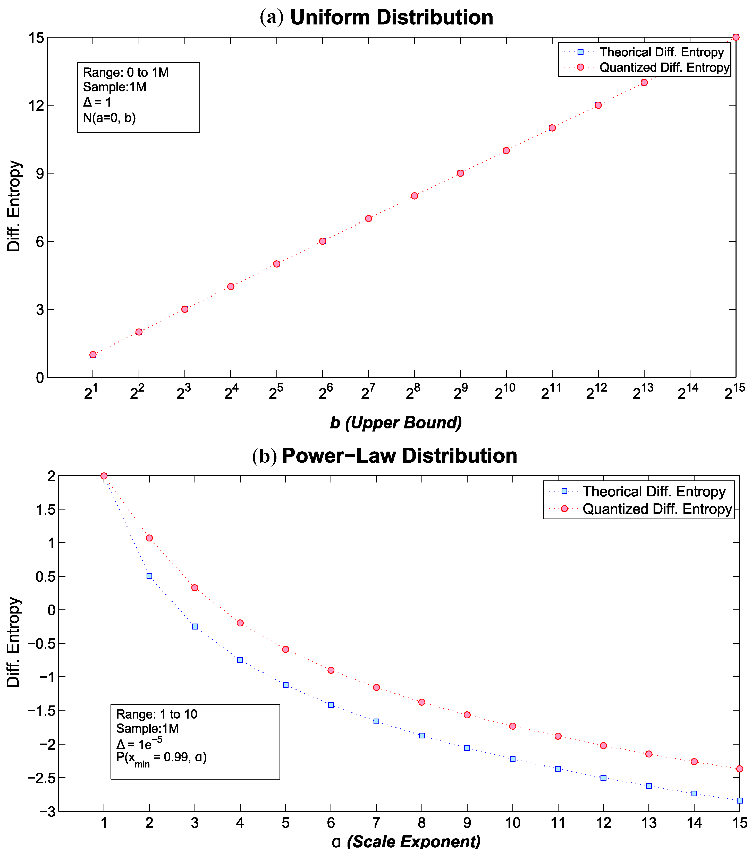
6.1.1. Uniform Distribution

The results for U were expected. We tested several values of the cardinality of P X , such that b = 2 i i = 1 , , 15 . Using the analytical H f formula of Table 1, the quantized H X Δ , and Δ = 1 , we achieved exactly the same differential entropy values. Results for U are shown in the left side of Figure 1. As was mentioned earlier, as the cardinality of the distribution grows, so does the differential entropy of U.

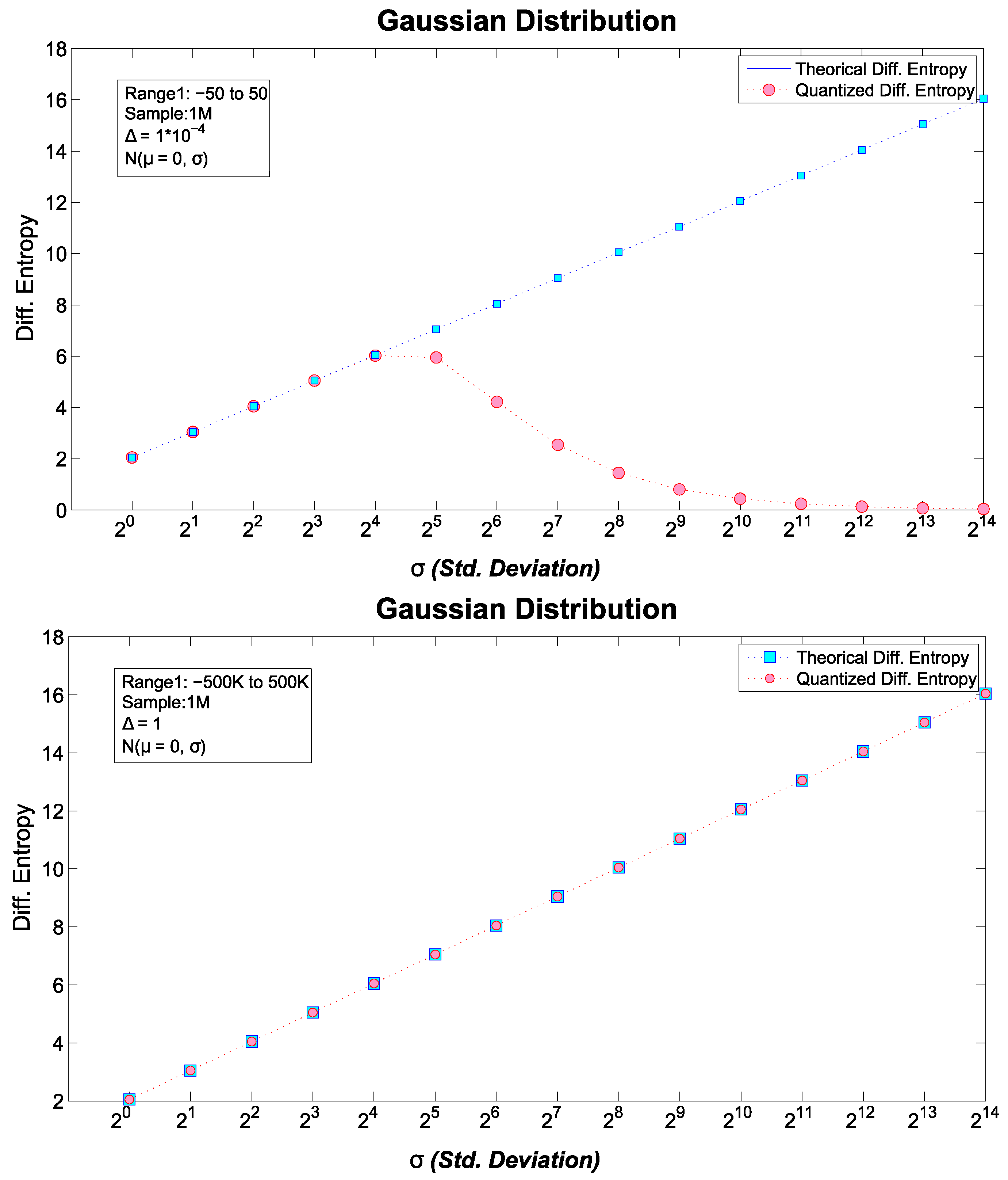
6.1.2. Normal Distribution

Results for the Gaussian distribution were less trivial. As in the U case, we calculate both H f and H X Δ , for a fixed μ = 0 , and modified the standard deviation parameter such that, σ = 2 i i = 0 , 1 , , 14 . Notice that the first tested distribution is the standard normal distribution.
In Figure 2, results obtained for the n-bit quantized differential entropy, and for the analytical form of Table 1 are shown. Moreover, we displayed two cases of the normal distribution: the left side of Figure 2 shows results for P X with range 50 , 50 and a bin size, Δ = 100 1 M = 1 × 10 4 , whereas, the right side provides results for a P X with range 500 e 3 , 500 e 3 and Δ = 1 . It is worth noting that, in the former case, the quantized differential entropy shows a discrepancy with H f after only σ = 2 4 = 16 , which quickly increases with growing σ. On the other hand, for the latter case, there is an almost perfect match between the analytical and quantized differential entropies; however, the same mismatch will be observed if the standard deviation parameter is allowed to grow unboundedly ( σ ) . Nonetheless, this is a consequence of how H X Δ is computed. As mentioned earlier, as Δ 0 , the value of each quantized X Δ grows towards . Therefore, in the G case, it seems convenient employing a Probability Mass Function (PMF) rather than a PDF. Consequently, the experimental setup of right side image of Figure 2 is employed for the calculation of the continuous complexity measures of G.

6.1.3. Power-Law Distribution
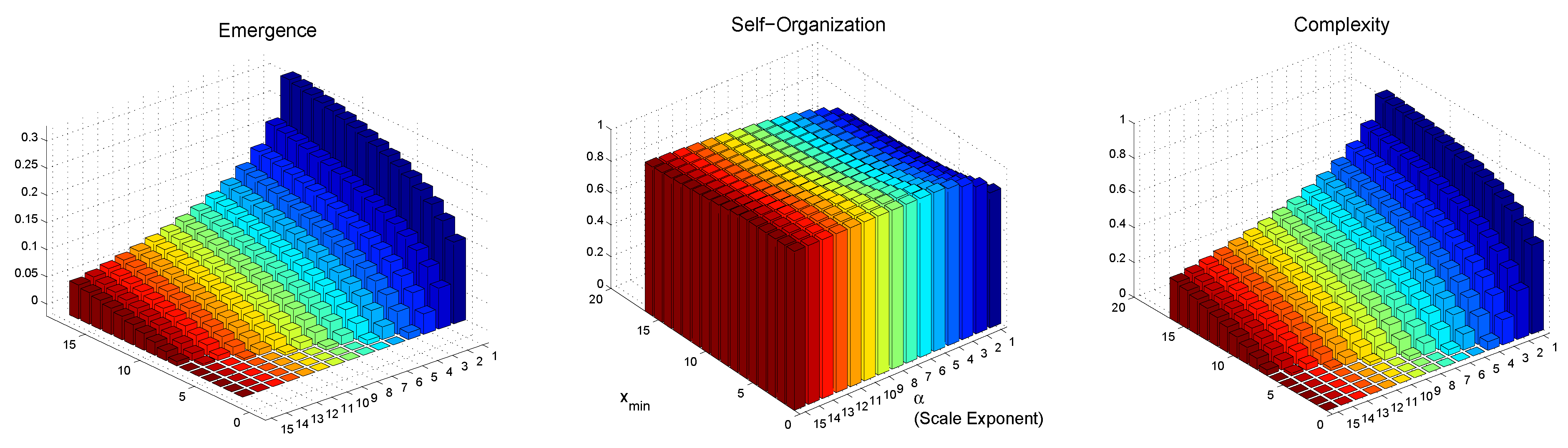
Results for the Power-Law distribution are shown in the right side of Figure 1. In both U and G, a PMF instead of a PDF was used to avoid cumbersome results (as depicted in the corresponding images). However, for the Power-Law distribution, the use of a PDF is rather convenient. As discussed in the next section and highlighted by [35], x m i n has a considerable impact on the value of H f . For Figure 1, the range employed was 1 , 50 , with a bin size of Δ = 1 × 10 5 , a x m i n = 0 . 99 , and modified the scale exponent parameter such that, α = i i = 1 , , 15 . For this particular setup, we can observe that as α increases, H f and H X Δ decreases its value towards . This effect is consequence of increasing the scale of the Power-Law such that, the slope of the function in a log-log space, approaches to zero. In this sense, with larger αs, the P X becomes closer to a Dirac delta distribution, thus, H f . However, as will be discussed later, for larger αs, larger x m i n values are required, in order for H f to display positive values.

6.2. Differential Complexity: E D , S D , and C D

U results are trivial: E D = 1 , and S D , C D = 0 . For each upper bound of U, E D = H U H U = 1 , which is exactly the same as its discrete counterpart. Thus, U results are not considered in the following analysis.
Continuous complexity results for G and PL are shown in Figure 3 and Figure 4, respectively. In the following, we provide details of these measures.

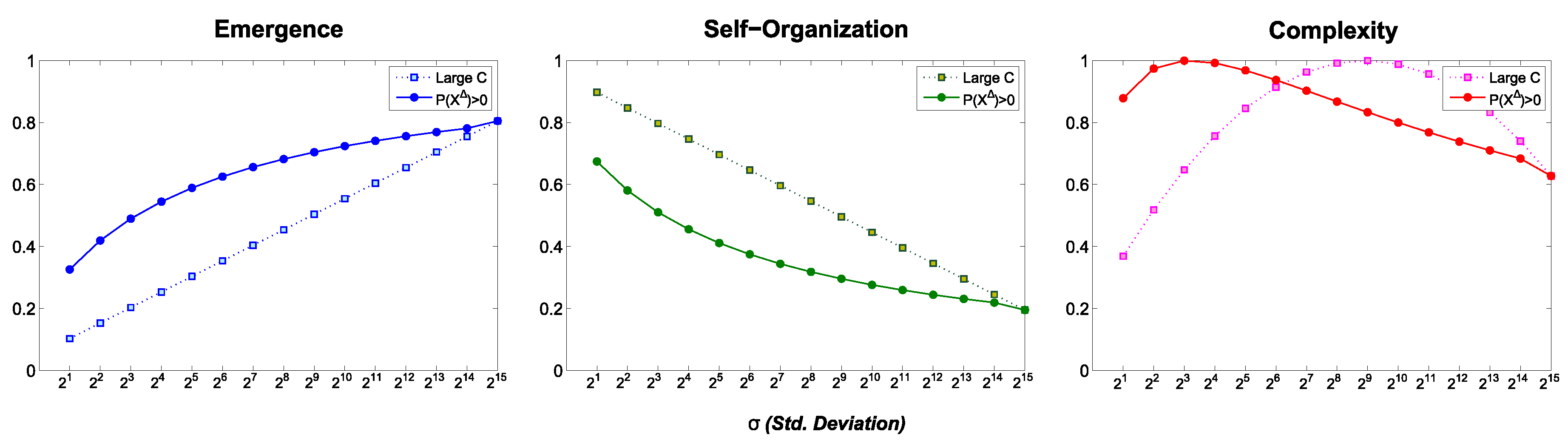
6.2.1. Normal Distribution

It was stated in Section 4 that the size of the alphabet is given by the function i n d P X . This rule establishes a valid cardinality such that P X > 0 , thus, only those states with a positive probability are considered. For P X Δ , such operation can be performed. Nevertheless, when the analytical H f is used, the proper cardinality of the set is unavailable. Therefore, in the Gaussian distribution case, we tested two criteria for selecting the value of b:
  • x i i n d · is employed for H X Δ .
  • A constant with a large value ( C = 1 × 10 6 ) is used for the analytical formula of H f .
In Figure 3, solid dots are used when K is equal to the cardinality of P X > 0 , whereas solid squares are used for an arbitrary large constant. Moreover, for the quantized case of P G , Table 2 shows the cardinality for each sigma, b i , and its corresponding K i . As can be observed, for a large normalizing constant K, a logarithmic relation is displayed for E D and S D . In addition, the maximum C D is achieved for σ = 2 8 = 256 , which is where E D = S D . However, for H X Δ the the maximum C D is found around σ = 2 1 , 2 , 3 = 2 , 4 , 8 , such that C D ϵ ϵ 0 . A word of advice must be made here. The required cardinality to normalize the continuous complexity measures such that 0 E D , S D , C D 1 , must have a lower bound. This bound should be related to the scale of the P X [40], and the quantization size Δ. In our case, when a large cardinality U = 1 × 10 6 , and Δ = 1 are used, the normalizing constant flattens E D results respect those obtained by b ; moreover, the large constant increases S D , and takes greater standard deviations for achieving the maximum C D . However, these complexity results are rather artificial in the sense that, if we arbitrarly let U then trivially we will obtain E D = 0 , S D = 1 , and C D = 0 . Moreover, it has been stated that the cardinality of P X should be employed as a proper size of b [26]. Therefore, when H X Δ is employed, the cardinality of P X > 0 must be used. On the contrary, when H f is employed, a coarse search for increasing alphabet sizes could be used so that the maximal H f satisfies H f H U 1 .

6.2.2. Power-Law Distribution

In this case, H f rather than H X Δ is used for computational convenience. Although the cardinality of P X > 0 is not available, by simply substituting p x i > 0 x = 1 , , 1 × 10 6 we can see that the condition is fulfilled by the whole set. Therefore, the large C criterium, earlier detailed, is used. Still, given that a numerical Power-Law distribution is given by two parameters, a lower bound x m i n and the scale exponent α, we depict our results in 3D in Figure 4. From left to right, E D , S D , and C D for the Power-Law distribution are shown, respectively. In the three images, the same coding is used: x-axis displays the scale exponent (α) values, y-axis shows x m i n values, and z-axis depicts the continuous measure values; lower values of α are displayed in dark blue, turning into reddish colors for larger exponents.
As it can be appreciated in Figure 4, for small x m i n (e.g., x m i n = 1 ) values, low emergence is produced despite the scale exponent. Moreover, maximal self-organization ( i.e. , S D = 1 ) is quickly achieved (i.e., α = 4 ), providing a PL with at most fair complexity values. However, if we let x m i n take larger numbers, E D grows, achieving the maximal complexity (i.e., C D 0 . 8 ) of this experimental setup at x m i n = 15 , α = 1 . This behavior is also observed for other scale exponent values, where emergence of new information is produced as the x m i n value grows. Furthermore, it has been stated that for P X , which displays a Power-Law behavior, it is required that x i P X x i > x m i n [37]. Thus, for every α there should be an x m i n such that E D > 0 . Moreover, for larger scale exponents, larger x m i n values are required for the distribution shows emergence of new information at all.

6.3. Real World Phenomena and Their Complexity

Data of phenomena that follows a Power-Law is provided in Table 3. These Power-Laws have been studied by [35,37,39], and the Power-Law parameters were published by [39]. The phenomena in the table mentioned above compromises data from:
  • Numbers of occurrences of words in the novel Moby Dick by Hermann Melville.
  • Numbers of citations to scientific papers published in 1981, from the time of publication until June 1997.
  • Numbers of hits on websites by users of America Online Internet services during a single day.
  • Number of received calls to A.T.&T. U.S. long-distance telephone services on a single day.
  • Earthquake magnitudes occurred in California between 1910 and 1992.
  • Distribution of the diameter of moon craters.
  • Peak gamma-ray intensity of solar flares between 1980 and 1989.
  • War intensity between 1816–1980, where intensity is a formula related to the number of deaths and warring nations populations.
  • Frequency of family names accordance with U.S. 1990 census.
  • Population per city in the U.S. in agreement with U.S. 2000 census.
More details about these Power-Laws can be found in [35,37,39].
For each phenomenon, the corresponding differential entropy and complexity measures are shown in Table 3. Furthermore, we also provide Table 4 which is a color coding for complexity measures proposed in [4]. Five colors are employed to simplify the different value ranges of E D , S D , and C D results. According to the nomenclature suggested in [4], results for these sets show that, very high complexity 0 . 8 C D 1 is obtained by the number of citations set (i.e., 2), and intensity of solar flares (i.e., 7). High complexity, 0 . 6 C D < 0 . 8 is obtained for received telephone calls (i.e., 4), intensity of wars (i.e., 8), and frequency of family names (i.e., 9). Fair complexity 0 . 4 C D < 0 . 6 is displayed by earthquakes magnitude (i.e., 5), and population of U.S. cities (i.e., 10). Low complexity, 0 . 2 C D < 0 . 4 is obtained for frequency of used words in Moby Dick (i.e., 1) and web hits (i.e., 3), whereas, moon craters (i.e., 6) have very low complexity 0 C D < 0 . 2 . In fact, earthquakes, and web hits, have been found not to follow a Power-Law [35]. Furthermore, if such sets were to follow a Power-Law, a greater value of x m i n would be required as can be observed in Figure 4. In fact, the former case is found for the frequency of words used in Moby Dick. In [39], parameters of Table 3 are proposed. However, in [35], another set of parameters are estimated (i.e., x m i n = 7 , α = 1 . 95 ). For the more recent estimated set of parameters, a high complexity is achieved (i.e., C D = 0 . 74 ), which is more consistent with literature about Zipf’s law [39]. Lastly, in the case of moon craters, the x m i n = 0 . 01 is rather a poor choice according to Figure 4. For the chosen scale exponent, it would require at least a x m i n 1 , for the Power-Law to produce any information at all. It should be noted that x m i n can be adjusted to change the values of all measures. In addition, it is worth mentioning that if we were to normalize and discretize a Power-Law distribution to calculate its discrete entropy (as in [4]), all Power-Law distributions present a very high complexity, independently of x m i n and α, precisely because these are normalized. Still, this is not useful for comparing different Power-Law distributions.

7. Discussion

In this paper, we extended complexity measures based on Shannon’s entropy to the continuous domain. Shannon’s continuous entropy cannot measure the average predictability of a system as its discrete counterpart. Rather, it measures the average uncertainty of a system given a configuration of a probability distribution function. Therefore, continuous Emergence, Self-organization, and Complexity describe the expected predictability of a system given it follows a probability distribution with a specific parameters set. It is common in many disciplines to describe real world systems using a particular probability distribution function. Therefore, the proposed measures can be useful to describe the production of information and novelty in such cases, or how information and uncertainty would change in the system if parameters were perturbed. Certainly, the interpretation of the measures is not given, as this will depend on the use we make of the measures for specific purposes.
From exploring the parameter space of the uniform, normal, and scale-free distributions, we can corroborate that high complexity values require a form of balance between extreme cases. On the one hand, uniform distributions, by definition, are homogeneous and thus all states are equiprobable, yielding the highest emergence. This is also the case of normal distributions with a very large standard deviation and for Power-Law distributions with an exponent close to zero. On the other hand, highly biased distributions (very small standard deviation in G or very large exponent in PL) yield a high self-organization, as few states accumulate most of the probability. Complexity is found between these two extremes. From the values of σ and α, this coincides with a broad range of phenomena. This does not tell us something new: complexity is common. The relevant aspect is that this provides a common framework to study of the processes that lead phenomena to have a high complexity [41]. It should be noted that this also depends on the time scales at which change occurs [42].
Many real-world phenomena are modelled under some probability distribution assumption. These impositions are rather a consequence of analytical convenience than intrinsic to the phenomenon under study. Nevertheless, these usually provide a rough but useful approximation for explanatory purposes: ranging from models of wind speed (Weibull distribution) to economic models (Logistic distribution), PDFs “effectively” describe phenomena data. Thus, in future work, it would be very useful to characterize PDFs like the Laplace, Logistic, and Weibull distribution to shed light in terms of complexity, emergence, and self-organization of systems, which can be modelled by these PDFs.
On the other hand, it is interesting to relate our results with information adaptation [17]. In a variety of systems, adaptation takes place by inflating or deflating information, so that the “right” balance is achieved. Certainly, given that it is possible to derive upper and lower bounds for the differential entropy of a PDF (e.g., [20]), it should be also possible to define analytical bounds for the complexity measures for the given PDF. However, for practical purposes, complexity measures are constrained by the selected range of the PDF parameters. Thus, the precise balance change from system to system and from context to context. Still, the capability of information adaptation has to be correlated with complexity, as the measure also reflects a balance between emergence (inflated information) and self-organization (deflated information).
As future work, it will be interesting to study the relationship between complexity and semantic information. There seems to be a connection with complexity as well, as we have proposed a measure of autopoiesis as the ratio of the complexity of a system over the complexity of its environment [4,43]. These efforts should be valuable in the study of the relationship between information and meaning, in particular in cognitive systems.
Another future line of research lies in the relationship between the proposed measures and complex networks [44,45,46,47], exploring questions such as: how does the topology of a network affect its dynamics? How much can we predict the dynamics of a network based on its topology? What is the relationship between topological complexity and dynamic complexity? How controllable are networks [48] depending on their complexity?

Acknowledgments

Guillermo Santamaría-Bonfil was supported by the Universidad Nacional Autónoma de México (UNAM) under grant CJIC/CTIC/0706/2014. Carlos Gershenson was supported by projects 212802 and 221341 from the Consejo Nacional de Ciencia y Tecnología, and membership 47907 of the Sistema Nacional de Investigadores of México.

Author Contributions

Guillermo Santamaría-Bonfil, Carlos Gershenson conceived and designed the experiments; Guillermo Santamaría-Bonfil performed the experiments; Guillermo Santamaría-Bonfil, Nelson Fernández and Carlos Gershenson wrote the paper. All authors have read and approved the final manuscript.

Conflicts of Interest

The authors declare no conflict of interest.

References

  1. Gershenson, C. (Ed.) Complexity: 5 Questions; Automatic Peess/VIP: Copenhagen, Denmark, 2008.
  2. Prokopenko, M.; Boschetti, F.; Ryan, A. An Information-Theoretic Primer on Complexity, Self-Organisation and Emergence. Complexity 2009, 15, 11–28. [Google Scholar] [CrossRef]
  3. Gershenson, C.; Fernández, N. Complexity and Information: Measuring Emergence, Self-organization, and Homeostasis at Multiple Scales. Complexity 2012, 18, 29–44. [Google Scholar] [CrossRef]
  4. Fernández, N.; Maldonado, C.; Gershenson, C. Information Measures of Complexity, Emergence, Self-organization, Homeostasis, and Autopoiesis. In Guided Self-Organization: Inception; Prokopenko, M., Ed.; Springer: Berlin/Heidelberg, Germany, 2014; Volume 9, pp. 19–51. [Google Scholar]
  5. Shannon, C.E. A mathematical theory of communication. Bell Syst. Tech. J. 1948, 27, 379–423, 623–656. [Google Scholar] [CrossRef]
  6. Gershenson, C.; Heylighen, F. When Can We Call a System Self-Organizing? In Advances in Artificial Life; Banzhaf, W., Ziegler, J., Christaller, T., Dittrich, P., Kim, J.T., Eds.; Springer: Berlin/Heidelberg, Germany, 2003; pp. 606–614. [Google Scholar]
  7. Langton, C.G. Computation at the Edge of Chaos: Phase Transitions and Emergent Computation. Physica D 1990, 42, 12–37. [Google Scholar] [CrossRef]
  8. Kauffman, S.A. The Origins of Order; Oxford University Press: Oxford, UK, 1993. [Google Scholar]
  9. Lopez-Ruiz, R.; Mancini, H.L.; Calbet, X. A statistical measure of complexity. Phys. Lett. A 1995, 209, 321–326. [Google Scholar] [CrossRef]
  10. Zubillaga, D.; Cruz, G.; Aguilar, L.D.; Zapotécatl, J.; Fernández, N.; Aguilar, J.; Rosenblueth, D.A.; Gershenson, C. Measuring the Complexity of Self-organizing Traffic Lights. Entropy 2014, 16, 2384–2407. [Google Scholar] [CrossRef]
  11. Amoretti, M.; Gershenson, C. Measuring the complexity of adaptive peer-to-peer systems. Peer-to-Peer Netw. Appl. 2015, 1–16. [Google Scholar] [CrossRef]
  12. Febres, G.; Jaffe, K.; Gershenson, C. Complexity measurement of natural and artificial languages. Complexity 2015, 20, 25–48. [Google Scholar] [CrossRef]
  13. Santamaría-Bonfil, G.; Reyes-Ballesteros, A.; Gershenson, C. Wind speed forecasting for wind farms: A method based on support vector regression. Renew. Energy 2016, 85, 790–809. [Google Scholar] [CrossRef]
  14. Fernández, N.; Villate, C.; Terán, O.; Aguilar, J.; Gershenson, C. Complexity of Lakes in a Latitudinal Gradient. Ecol. Complex. 2016. submitted. [Google Scholar]
  15. Cover, T.; Thomas, J. Elements of Information Theory; John Wiley Sons: Hoboken, NJ, USA, 2005; pp. 1–748. [Google Scholar]
  16. Michalowicz, J.; Nichols, J.; Bucholtz, F. Handbook of Differential Entropy; CRC Press: Boca Raton, FL, USA, 2013; pp. 19–43. [Google Scholar]
  17. Haken, H.; Portugali, J. Information Adaptation: The Interplay Between Shannon Information and Semantic Information in Cognition; Springer: Berlin/Heideberg, Germany, 2015. [Google Scholar]
  18. Heylighen, F.; Joslyn, C. Cybernetics and Second-Order Cybernetics. In Encyclopedia of Physical Science & Technology, 3rd ed.; Meyers, R.A., Ed.; Academic Press: New York, NY, USA, 2003; Volume 4, pp. 155–169. [Google Scholar]
  19. Ashby, W.R. An Introduction to Cybernetics; Chapman & Hall: London, UK, 1956. [Google Scholar]
  20. Michalowicz, J.V.; Nichols, J.M.; Bucholtz, F. Calculation of differential entropy for a mixed Gaussian distribution. Entropy 2008, 10, 200–206. [Google Scholar] [CrossRef]
  21. Calmet, J.; Calmet, X. Differential Entropy on Statistical Spaces. 2005; arXiv:cond-mat/0505397. [Google Scholar]
  22. Yeung, R. Information Theory and Network Coding, 1st ed.; Springer: Berlin/Heideberg, Germany, 2008; pp. 229–256. [Google Scholar]
  23. Bedau, M.A.; Humphreys, P. (Eds.) Emergence: Contemporary Readings in Philosophy and Science; MIT Press: Cambridge, MA, USA, 2008.
  24. Anderson, P.W. More is Different. Science 1972, 177, 393–396. [Google Scholar] [CrossRef] [PubMed]
  25. Shalizi, C.R. Causal Architecture, Complexity and Self-Organization in Time Series and Cellular Automata. Ph.D. thesis, University of Wisconsin, Madison, WI, USA, 2001. [Google Scholar]
  26. Singh, V. Entropy Theory and its Application in Environmental and Water Engineering; John Wiley Sons: Chichester, UK, 2013; pp. 1–136. [Google Scholar]
  27. Gershenson, C. The Implications of Interactions for Science and Philosophy. Found. Sci. 2012, 18, 781–790. [Google Scholar] [CrossRef]
  28. Sharma, K.; Sharma, S. Power Law and Tsallis Entropy: Network Traffic and Applications. In Chaos, Nonlinearity, Complexity; Springer: Berlin/Heidelberg, Germany, 2006; Volume 178, pp. 162–178. [Google Scholar]
  29. Dover, Y. A short account of a connection of Power-Laws to the information entropy. Physica A 2004, 334, 591–599. [Google Scholar] [CrossRef]
  30. Bashkirov, A.; Vityazev, A. Information entropy and Power-Law distributions for chaotic systems. Physica A 2000, 277, 136–145. [Google Scholar] [CrossRef]
  31. Ahsanullah, M.; Kibria, B.; Shakil, M. Normal and Student’s t-Distributions and Their Applications. In Atlantis Studies in Probability and Statistics; Atlantis Press: Paris, France, 2014. [Google Scholar]
  32. Box, G.; Jenkins, G.; Reinsel, G. Time Series Analysis: Forecasting and Control, 4th ed.; John Wiley Sons: Hoboken, NJ, USA, 2008. [Google Scholar]
  33. Mitzenmacher, M. A Brief History of Generative Models for Power Law and Lognormal Distributions. 2009; arXiv:arXiv:cond-mat/0402594v3. [Google Scholar]
  34. Mitzenmacher, M. A brief history of generative models for Power-Law and lognormal distributions. Internet Math. 2001, 1, 226–251. [Google Scholar] [CrossRef]
  35. Clauset, A.; Shalizi, C.R.; Newman, M.E.J. Power-Law Distributions in Empirical Data. SIAM Rev. 2009, 51, 661–703. [Google Scholar] [CrossRef]
  36. Frigg, R.; Werndl, C. Entropy: A Guide for the Perplexed. In Probabilities in Physics; Beisbart, C., Hartmann, S., Eds.; Oxford University Press: Oxford, UK, 2011; pp. 115–142. [Google Scholar]
  37. Virkar, Y.; Clauset, A. Power-law distributions in binned empirical data. Ann. Appl. Stat. 2014, 8, 89–119. [Google Scholar] [CrossRef]
  38. Yapage, N. Some Information measures of Power-law Distributions Some Information measures of Power-law Distributions. In Proccedings of the 1st Ruhuna International Science and Technology Conference, Matara, Sri Lanka, 22–23 January 2014.
  39. Newman, M. Power laws, Pareto distributions and Zipf’s law. Contemp. Phys. 2005, 46, 323–351. [Google Scholar] [CrossRef]
  40. Landsberg, P. Self-Organization, Entropy and Order. In On Self-Organization; Mishra, R.K., Maaß, D., Zwierlein, E., Eds.; Springer: Berlin/Heidelberg, Germany, 1994; Volume 61, pp. 157–184. [Google Scholar]
  41. Gershenson, C.; Lenaerts, T. Evolution of Complexity. Artif. Life 2008, 14, 241–243. [Google Scholar] [CrossRef] [PubMed]
  42. Cocho, G.; Flores, J.; Gershenson, C.; Pineda, C.; Sánchez, S. Rank Diversity of Languages: Generic Behavior in Computational Linguistics. PLoS ONE 2015, 10. [Google Scholar] [CrossRef]
  43. Gershenson, C. Requisite Variety, Autopoiesis, and Self-organization. Kybernetes 2015, 44, 866–873. [Google Scholar]
  44. Newman, M.E.J. The structure and function of complex networks. SIAM Rev. 2003, 45, 167–256. [Google Scholar] [CrossRef]
  45. Newman, M.; Barabási, A.L.; Watts, D.J. (Eds.) The Structure and Dynamics of Networks; Princeton University Press: Princeton, NJ, USA, 2006.
  46. Boccaletti, S.; Latora, V.; Moreno, Y.; Chavez, M.; Hwang, D.U. Complex networks: Structure and dynamics. Phys. Rep. 2006, 424, 175–308. [Google Scholar] [CrossRef]
  47. Gershenson, C.; Prokopenko, M. Complex Networks. Artif. Life 2011, 17, 259–261. [Google Scholar] [CrossRef] [PubMed]
  48. Motter, A.E. Networkcontrology. Chaos 2015, 25, 097621. [Google Scholar] [CrossRef] [PubMed]
Figure 1. Theoretical and quantized differential entropies for (a) Uniform distribution and (b) Power-Law distributions .
Entropy 18 00072 g001
Figure 2. Two comparisons of theoretical vs. quantized differential entropy for the Gaussian distribution.
Entropy 18 00072 g002
Figure 3. Complexity of the Gaussian distribution.
Entropy 18 00072 g003
Figure 4. Complexity measures for the Power-Law. Lower values of the scale exponent α are displayed in dark blue, colors turns into reddish for larger scale exponents.
Entropy 18 00072 g004
Table 1. Studied PDFs with their corresponding analytical differential entropies.
DistributionPDFDifferential Entropy
Uniform p x = 1 b a a x b 0 otherwise H p x = log 2 b
Normal p x = 1 σ 2 π e x μ 2 2 σ H p x = 1 2 log 2 2 π e σ 2
Power-law p x = α 1 x m i n x x m i n α H p x = log 2 x m i n log 2 α 1 + α α 1
Table 2. Alphabet size b , and its corresponding normalizing K constant for the normal distribution G.
σ b = i n d P r X > 0 H U = log 2 b K = 1 H U
2 0 = 1 786.280.16
2 1 = 2 1547.260.14
2 2 = 4 3088.270.12
2 3 = 8 6169.270.11
2 4 = 16 123210.270.10
2 5 = 32 246411.270.09
2 6 = 64 492412.270.08
2 7 = 128 984413.270.075
2 8 = 256 19,68014.260.0701
2 9 = 512 39,34015.260.0655
2 10 = 1024 78,64416.260.0615
2 11 = 2048 157,21217.260.058
2 12 = 4096 314,27818.260.055
2 13 = 8192 628,25819.260.0520
2 14 = 16 , 384 1,000,00019.930.050
Table 3. Power-Law parameters and information-based measures of real world phenomena.
Phenomenon x m i n α (Scale Exponent) H f E D S D C D
1Frequency of use of words12.21.570.0780.920.29
2Number of citations to papers1003.047.10.360.640.91
3Number of hits on web sites12.41.230.060.940.23
4Telephone calls received102.224.850.240.760.74
5Magnitude of earthquakes3.83.042.380.120.880.42
6Diameter of moon craters0.013.14 6 . 27 010
7Intensity of solar flares2001.8310.110.510.490.99
8Intensity of wars31.804.150.210.790.66
9Frequency of family names100001.9415.440.780.220.7
10Population of U.S. cities400002.3016.670.830.170.55
Table 4. Color coding for E D , S D , and C D results.
CategoryVery HighHighFairLowVery Low
Range [ 0 . 8 , 1 ] [ 0 . 6 , 0 . 8 ) [ 0 . 4 , 0 . 6 ) [ 0 . 2 , 0 . 4 ) [ 0 , 0 . 2 )
ColorBlueGreenYellowOrangeRed

