
Intransitivity in Theory and in the Real World

School of Mechanical and Mining Engineering, The University of Queensland, Brisbane QLD 4072, Australia
Entropy 2015, 17(6), 4364-4412; https://doi.org/10.3390/e17064364
Submission received: 30 March 2015
/
Revised: 2 June 2015
/
Accepted: 15 June 2015
/
Published: 19 June 2015
(This article belongs to the Special Issue Entropy, Utility, and Logical Reasoning)
Abstract
:This work considers reasons for and implications of discarding the assumption of transitivity—the fundamental postulate in the utility theory of von Neumann and Morgenstern, the adiabatic accessibility principle of Caratheodory and most other theories related to preferences or competition. The examples of intransitivity are drawn from different fields, such as law, biology and economics. This work is intended as a common platform that allows us to discuss intransitivity in the context of different disciplines. The basic concepts and terms that are needed for consistent treatment of intransitivity in various applications are presented and analysed in a unified manner. The analysis points out conditions that necessitate appearance of intransitivity, such as multiplicity of preference criteria and imperfect (i.e., approximate) discrimination of different cases. The present work observes that with increasing presence and strength of intransitivity, thermodynamics gradually fades away leaving space for more general kinetic considerations. Intransitivity in competitive systems is linked to complex phenomena that would be difficult or impossible to explain on the basis of transitive assumptions. Human preferences that seem irrational from the perspective of the conventional utility theory, become perfectly logical in the intransitive and relativistic framework suggested here. The example of competitive simulations for the risk/benefit dilemma demonstrates the significance of intransitivity in cyclic behaviour and abrupt changes in the system. The evolutionary intransitivity parameter, which is introduced in the Appendix, is a general measure of intransitivity, which is particularly useful in evolving competitive systems.
1. Introduction
The strongest case for the existence of methodological similarity between utility and entropy is represented by two fundamental results: (a) the utility theory of von Neumann and Morgenstern [1] and (b) introduction of entropy through the adiabatic accessibility principle of Caratheodory [2]. The latter approach was rigorously formalised by Lieb and Yngvason [3]. The physical interpretation of this mathematical theory is linked to the so-called weight process previously suggested by Gyftopoulos and Beretta [4]. Both of these theories link ordering of states to a ranking quantity (utility U or entropy S) and are based on two fundamental principles:
- Transitivity
- Linearity (in thermodynamics: extensivity) implying that
In Equation (1), the overall lottery is a combination of two outcomes A an B with utilities uA and uB and probabilities PAand PB. In Equation (2), the overall system is a combination of two subsystems A an B with specific entropies sA and sB and masses mAand mB.
While the similarity between utility and entropy is obvious, this similarity remains methodological: theories a and b are generally applied to different objects taken from different fields of science. There are however some exceptions, such as competitive systems [5–7]. These systems incorporate competition preferences and, at the same time, permit thermodynamic considerations (here we refer to apparent thermodynamics—using approaches developed in physical thermodynamics and statistical physics to characterise systems not related to heat and engines).
Further investigations into human decision-making under risk have revealed substantial disagreements with von Neumann–Morgenstern utility theory, indicating that preferences depend non-linearly on probabilities. One of the most prominent examples demonstrating non-linearity of human preferences is known as the Allais paradox [8]. A spectrum of generalisations introducing utilities that are non-linear with respect to probabilities has appeared [9–12], most notably the cumulative prospect theory [13]. In thermodynamics, generalisations of conventional entropy have brought new formulations for non-extensive entropies [14], most notably Tsallis entropy [15] and its modifications [16]. Physically, the definitions of non-extensive entropies correspond to the existence of substantial stochastic correlations between subsystems. All of these theories do not violate or question the first fundamental principle listed above—transitivity.
In this work, we are interested in the phenomenon of intransitivity, i.e., violations of transitivity. A good example of intransitivity has been known for a long time under the name of the Condorcet paradox [17]. The existence of intransitivity in human preferences has been repeatedly suggested [18–20] and has its advocates and critics. The main argument against intransitivity is its perceived irrationality [21], which was disputed by Anand [22] from a philosophical perspective. Critics of intransitivity often argue that “abolishing” transitivity is wrong as we need utility and entropy, while these quantities are linked to transitivity. The question, however, is not merely in the replacement of one assumption by its negation: while transitivity is a reasonable assumption in many good theories, its limitations are a barrier for explaining the complexity of the surrounding world. Both transitive and intransitive effects are common and need to be investigated irrespective of what we tend to call “rational” or “irrational”. As discussed in this work, intransitivity appears under a number of common conditions and, therefore, must be ubiquitously present in the real world. We have all indications that intransitivity is a major factor stimulating emergence of complexity in the competitive world surrounding us [5,6]. It is interesting to note that the presence of intransitivity is acknowledged in some disciplines (e.g., population biology) but is largely overlooked in others (e.g., economics). This work is intended as a common platform for dealing with intransitivity across different disciplines.
Sections 2, 6 and 8 and Appendices present a general analysis. Sections 3–5 and 7 present examples from game theory, law, ecology and behavioral economics. Section 9 presents competitive simulations of the risk/benefit dilemma. Section 10 discusses thermodynamic aspects of intransitivity. Concluding remarks are in Section 11.
2. Preference, Ranking and Co-Ranking
This section introduces main definitions that are used in the rest of the paper. The basic notion used here is preference, which is denoted by the binary relation A≺B, or equivalently by B≻A, implying that element B has some advantage over element A. In the context of a competitive situation, A≺B means that B is the winner in competition with A. The notation A⪯B indicates that either element B is preferred over element A (i.e., A≺B), or the elements are equivalent (i.e., A∼B, although A and B are not necessarily the same A≠B). The elements are assumed to be comparable to each other (i.e., possess relative characteristics), while absolute characteristics of the elements may not exist at all or remain unknown. If equivalence (indifference) A∼B, is possible only when A=B then this preference is called strict.
The preference is transitive when
for any three elements A, B and C. Otherwise, existence of at least one intransitive triplet
indicates intransitivity of the preference. Generally, we need to distinguish current transitivity—i.e., transitivity of preference on the current set of elements—from the overall transitivity of the preference rules (if such rules are specified): the latter requires the former but not vice versa. Intransitive rules may or may not reveal intransitivity on a specific set of elements. Intransitivity is called potential if it can appear under considered conditions but may or may not be revealed on the current set of elements.
2.1. Co-Ranking
The preference of B over A can be equivalently expressed by a co-ranking function ρ(B,A) so that
This implies the following functional form for co-ranking:
By definition, co-ranking is antisymmetric:
Co-ranking is a relative characteristic that specifies properties of one element with respect to the other, while absolute characteristics of the elements may not exist or be unknown. Co-ranking can be graded, when the value ρ(B,A) is indicative of the strength of our preference, or sharp otherwise. Generally we presume graded co-ranking. However, a graded co-ranking may or may not be specified (and exist) for a given preference. If ranking is sharp, only the sign of ρ(B,A) is of interest while the magnitude ρ(B,A) is an arbitrary value. The following definition of the indicator co-ranking
corresponds to information available in sharp preferences. The indicator co-ranking R is a special case of co-ranking ρ. The function R(B,A) can be also called the indicator function of the preference.
2.2. Absolute Ranking
If the preference is transitive, it can be expressed with the use of a numerical function r(…) called absolute ranking so that
for any A and B. (We consider mainly discrete systems but, in the case of continuous distributions, the existence of absolute rankings for transitive preferences is subject to the conditions of the Debreu theorem [23] (i.e., continuity of the preferences), which are presumed to be satisfied in this work.) Ranking is called strict when the corresponding preference is strict (i.e., r(A) = r(B) demands A=B). As with co-rankings, we distinguish graded and sharp rankings. In the case of the sharp ranking, the value r(B) − r(A) > 0 tells us only that B is better than A but, generally, does not give any indication of the magnitude of our preference. From a mathematical perspective, a sharp ranking represents a total pre-ordering of the ranked elements, while a sharp strict ranking represents an ordering. Any strictly monotonic function fm(…) of a sharp ranking is still an equivalent ranking fm(r(…)) ∼ r(…) with the same ordering. In the case of the graded ranking, the value r(B) − r(A) represents the magnitude of our preference of B over A. In many cases, a graded ranking corresponds to a physical quantity that can be directly determined or measured. In economics, graded rankings are called utility, in biology graded rankings are called fitness, in thermodynamics graded rankings correspond to entropy. Here, we follow the notation of economics and, when applicable, refer to graded rankings as utility. Practically, the line between sharp and graded rankings is blurred. It is often the case that even a nominally sharp ranking can give some indication of the magnitude of the preference, for example, in terms of the density of elements. Different rankings (or co-rankings) are called equivalent if they correspond to the same preference (but might still can have different preference magnitudes).
If a co-ranking specifies a transitive preference, there exists an absolute ranking for this preference (which is not unique). The absolute ranking induces a co-ranking, which is linked to the absolute ranking by the relation
and referred to as the absolutely transitive co-ranking. By definition, the original co-ranking is equivalent to co-ranking Equation (10) but does not necessarily coincide with it indicating different magnitude of the preference. The co-rankings defining intransitive preferences are called intransitive, while co-rankings that define transitive preferences on a given set of elements but cannot be represented by Equation (10) are called potentially intransitive as intransitivity can appear for these co-rankings under conditions specified in Appendix A.
2.3. Average Rankings
We are interested in ranking element A with respect to a group of elements (that may or may not include A), say, group G represented by a set S of elements Ci ∈
and the corresponding weights gi = g(Ci) > 0, while g(Cj) = 0 for Cj ∉
. We can also write Ci ∈
implying that Ci ∈
. The average co-ranking of element A and group
, is defined by the equation
where G is the total weight of the group
Note that
. If all weights are the same gi = 1 within the group, then G is the number of elements in the group and the meanings of
and
are essentially the same while the terms “set” and “group” become interchangable (i.e., specification
as a set implies unit weights for the elements). The co-ranking ρ(A,Ci) and corresponding preference are referred to as underlying co-ranking and preference of the ranking
, while the preference
is called the preference induced by the ranking
. The ranking
and the preference induced by
are called conditional indicating conditioning of ranking on
. The group
and weights gi are called the reference group and reference weights.
The co-ranking of two groups
and
, which is called group co-ranking, is defined in the same way
where g′ and g′ are the weights and G′ and G″ are the total weights associated with the groups
and
. In case of continuous distributions, the sums are to be replaced by the corresponding integrals.
If the underlying preference is specified by an absolutely transitive co-ranking (as represented by Equation (10)), then we can write for the average co-ranking
and
where
is the average absolute ranking of group
.
Proposition 1 All conditional rankings indicate the same magnitude of preference, i.e.,
for any A, B∈
and any,
⊂
, if and only if the underlying co-rankings are absolutely transitive.
Equation (15) demonstrates validity of the direct part of the proposition
The inverse part can be shown by considering groups represented by one-element sets
and
. Then Equation (18) becomes
and in, particular, if D = B then ρ(A,B) = ρ(A,C) − ρ(B,C) for all A, B and C. Hence, we can define absolute ranking by the following relation:
for arbitrary B and fixed A.
Proposition 2 If the preferences induced by all conditional rankings are equivalent, i.e.,
for any A,B∈
and any,
⊂
, then the underlying preference is currently transitive.
We consider intransitive triplet (4) (i.e., A⪯B⪯C≺A)—there must be at least one if the preference is intransitive—and demonstrate that at least some of the conditional rankings are different. For two one-element groups
and
, we, obviously, have 0 ≥ ρ{B} (A) ≤ ρ{B} (C) ≥ 0 but 0 < ρ{C} (A) > ρ{C} (C) = 0. Hence, the following conditional preferences
are different. This contradicts (22) implying that the underlying preference must be transitive.
Hence, if a binary preference is specified, elements in a given set can always be ordered transitively by conditional ranking of the elements with respect to a selected reference group or set (which may or may not coincide with the given set). If the original preference is transitive, it uniquely determines the ordering irrespective of the reference group. If the original preference is intransitive, then the relative positions of at least two elements in this ordering (with respect to each other: say A before B or A after B) depend on the presence of the other elements in the reference set.
Conditional ranking and group co-ranking can also be introduced for the indicator co-ranking
which are distinguished by using the word “indicator”. For example, conditional indicator co-rankings are further discussed in Appendix B. Note that the group preferences induced by the indicator co-rankings
can be intransitive even if the underlying element preference is currently transitive (see Proposition B3). All co-rankings and conditional rankings (such as ρ, R,
,
,
,
) are relative as opposite to the absolute ranking of the previous subsection.
2.4. Is Intransitivity Irrational?
Preferences are always attached to specific conditions and can become illogical or contradictory if taken out of context and this work endeavors to use examples to illustrate this point. The propositions of the previous subsections demonstrate that intransitivity is associated with relativistic views. The choice between transitive (absolute) and intransitive (relativistic) models depends on nature of the processes that these models are expected to reproduce. Many people, however, have psychological difficulties in accepting a relativistic approach, expecting an absolute scale of judgments from “bad” to “good”, which can be suitable in some cases but excessively simplistic in the others.
The argument for irrationality of intransitivity [21] is based on the alleged impossibility of choosing between A, B and C when A≺B, B≺C and C≺A. It is often suggested that in this case a decision maker will circle between these thee options indefinitely, which is impossible or open to numerous contradictions. In fact, binary preferences determine the selection of a single element from pairs, but do not tell us how the choice should be performed when all three elements are simultaneously present in the current set of {A,B,C}. This can be achieved consistently on the basis of the conditional ranking
, where
. It might be the case that
but this case is no more illogical than selecting from a set with transitive preferences and equivalent elements, e.g., A∼B∼C∼A. While identifying the reference set with the current set is most obvious choice in absence of additional information, deploying alternative reference sets is also possible in practical situations. For example, a buyer may use information about popularity of different models instead of considering the set of models currently available in the store. In a generic consideration of this subsection, we follow the logical choice of identifying the reference set with the current set and setting the reference weights to unity.
The preference between elements A and B selected from the current set of {A,B} is based on the conditional ranking
as specified by Equation (11) with gi = 1. The conditional co-ranking, which is a measure of conditional preference of A over B introduced by similarity with Equation (10), becomes
This is expected: ρ(A,B) indicates a preference between A and B when selected from the set of {A,B}. Let us compare this to preferences between A and B when the current (reference) set has three elements {A,B,C}. The conditional ranking is now specified by
with the corresponding conditional co-ranking
where
are introduced. In absolutely transitive cases, ρ{C}(A,B) = ρ(A,B), δ(C,B,A) = 0 and ρ{A,B,C} (A,B) is the same as ρ(A,B). However, ρ{A,B,C}(A,B) and ρ(A,B) are not necessarily equivalent in intransitive cases. The combination of intransitivity with a presumption of invariance of conditional rankings, which is incorrect in intransitive cases, may result in logical contradictions. In a consistent approach, the specification of preference between A and B for selection from the set of {A,B,C} should be ρ{A,B,C}(A,B) and not ρ(A,B).
If only relative characteristics (i.e., co-ranking but not absolute ranking) are specified or known, the preferences defined by these characteristics are most likely to be intransitive or potentially intransitive. The case of absolutely transitive co-rankings is a very specific case and, in general, cannot be presumed a priori. The existence of a transitive ordering can simplify choices but “simpler” does not necessarily mean “more accurate” or “more realistic”. Intransitivity is not irrational, but considering intransitivity while neglecting relativistic nature of conditional preferences is illogical and can lead to contradictions. The examples of the following sections show that our preferences are indeed relativistic and, generally, intransitive but this is often (and incorrectly) seen as “irrationality”, which is not amendable to logical analysis.
3. Intransitivity and Game Theory
3.1. Games with Explicit Intransitivity
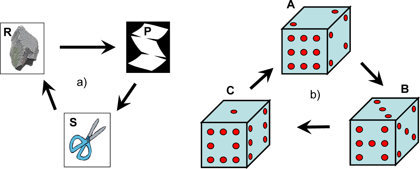
Games with explicit intransitivity involve preset rules that a priori specify intransitive preferences. The best-known example of such games is the rock(R)-paper(P)-scissors(S) game. The rules of this game are expressed by the intransitive preference R≺P≺S≺R, which is illustrated in Figure 1a. The players
and
independently select one of the options (pure strategies) R, P or S and the winner is determined by the specified preference. Obviously, intransitive rules are related to intransitive strategies. Indeed, if a player has to select between two options, while the remaining option has to be taken by the opponent, the player would obviously prefer P to R, S to P and R to S. Hence, appearance of intransitive strategies in explicitly intransitive games is natural and common.
In a more general case, consider players
and
who select options (pure strategies) C1,C2, … from the respective subsets
and
of set
with respective probabilities
and
. The sets
and
may overlap. Hence, the players’ selections are represented by groups
and
. Player
chooses group
while player
chooses group
but the players are not allowed to change the subsets
and
. Any Ci ∈
is called available to player
, while any Ci ∈
is called selected by player
. The relative strength of pure strategies Ci and Cj, which is called payoff in game theory, is determined by co-ranking ρ(Ci,Cj). This defines a general zero-sum game for two players,
and
, while the groups
and
represent mixed strategies of the players. It is easy to see that the overall payoff of the game is determined by
Here, the average co-ranking
is defined by Equation (14) but the total weights are taken
since
and
are interpreted as probabilities. If
and
are distinct, then the rules of the game might define only preferences between elements from different sets
and
but not within each set. If these preferences can be extended transitively to all possible pairs from
, then the rules of the game are seen as being transitive (and are intransitive otherwise).
The mixed strategies of this game are known to possess Nash equilibrium [24], where change of the mixed strategy by each player does not increase his overall payoff, assuming that mixed strategies of the remaining player stay the same. This condition can be expressed in terms of conditional rankings defined by Equation (11):
Proposition 3 (Nash [24]) Nash equilibrium is achieved when and only when all options in a mixed strategy selected by each player have maximal (and the same within each mixed strategy) ranking conditioned on the mixed strategy of the opposition:
Indeed, if there was A ∈
with
then player
can improve his overall payoff by setting g0(A) = 0 and eliminating A from G0. In this proposition,
is understood as any of the two players and
represents his opposition. Note that, generally,
, where
If the preferences between strategies and the associated co-rankings are absolutely transitive, then Nash equilibrium is achieved when each player selects the option(s) with the highest absolute ranking in the set available to the player. Transitive games are relatively simple and are not particularly interesting. Finding Nash equilibrium in case of a game with intransitive preferences can be more complicated.
For example, in the rock-paper-scissors game with all options available to all players (i.e.,
), the Nash equilibrium is specified by
with all conditional rankings being the same
and the overall payoff of
If player
alters his mixed strategy
(while
does not change), the overall payoff of the game remains the same. However, any strategy of
that is different from
specified by Equation (34) can be exploited by player
to get a better payoff for
.
3.2. Games with Potential Intransitivity
Some games have rules that do not explicitly stipulate intransitive relations but allow for optimal intransitive strategies. Consider a game where two dice are thrown and the one which shows a greater number wins—there is nothing explicitly intransitive in these rules (and an example of a transitive set of dice can be easily suggested). However, the dice shown in Figure 1b are clearly intransitive. In accordance with the terminology used in this work, we call these games potentially intransitive. Determining existence of intransitive optimal strategies in a particular potentially intransitive game can be complicated.
It has been noticed that an ordinary cat tends to prefer fish to meat, meat to milk, and milk to fish [25]. Makowski and Piotrowski [25–27] considered a number of models that can explain these intransitive preferences by the perfectly rational need of balancing cat’s diet. These models include a classical cat [26] and a quantum cat [25], and are sufficiently general to be applied to other problems such as adversarial/cooperative balanced food games [27] or to choosing candidates in elections [28] (quantum preferences are briefly discussed in Appendix F). In these models, a cat is offered three types of food in pairs with some probabilities and is forced to chose between them. The cat strives to achieve a perfect balanced diet and can follow various strategies (transitive or intransitive), while intransitivity is not enforced in any way on the cat by the game rules. The main conclusion drawn by Makowski and Piotrowski [27] is consistent with the approach taken in this work: intransitive strategies can be not only perfectly rational but also the best under certain conditions (while in other circumstances transitive strategies are optimal). Choosing between transitive and intransitive strategies is no more than one of the attributes in selecting the best tactics under given circumstances—this choice is not linked to upholding rationality of modern science.
4. Example: Intransitivity of Justice
The possibility of intransitivity in legal regulations has been noticed and discussed in several publications [29,30]. In this section, we offer a different example of intransitivity and suggest some interpretations.
Consider the following options available to people witnessing a fire:
- (A) Doing nothing;
- (B) Calling the fire service;
- (C) Trying to rescue people from the fire and/or extinguish the fire
4.1. Popular View
One can guess that popular (and, possibly, somewhat naive) estimate for utility of these options would be
implying that people think of option C as having a higher value for society than option B (As a proof, I recall my childhood experienmce: after extinguishing a faulty camp stove engulfed by flames my father became a local celebrity among other holidaymakers. I am sure that his treatment would be less favirouble if, instead, he limited his actions to hitting a firealarm button). This popular treatment of the choice between options A, B and C, which is shown in Figure 2 by dashed line is perfectly transitive and self-consistent
The corresponding conditional indicator co-ranking with respect to the reference set of
is determined by Equation (24) and given by
4.2. Treatment by Law: Can Do More but not Less
Let us examine how the same choice, when made by an employee in the case of a fire in a work environment, is treated by law. The law expects that the employee either must rush to call the fire service or can do more by trying to extinguish the fire. Hence A≺B—the employee must chose B over A, if only two options A and B are available to him. The employee is free to chose between B and C (i.e., B∼C). The law, however, does not demand that the employee risks his life if the choice is to be made between A and C (i.e., C∼A). One can see that this treatment of the options is intransitive
and corresponds to the following indicator co-ranking
which is illustrated in Figure 2a. Note that the intransitivity of Equation (40) is weak—it violates only transitivity of equivalence. If the choice is to be made between three options, then B and C are legal while A is not. This implies the following ordering [{B,C}, A] (here, the square brackets denote ordered sets).
The indicator co-ranking conditioned on the reference set of
indicates something that we might have guessed already: legally, B is the safest option. Note that the legal Equation (42) and common Equation (37) systems of values may differ. The law prefers option B, tolerates option C and objects to option A so that the three options, when are ordered according to likely legal advice, are listed as [B,C,A] (although, as noted above, options B and C are legal while A is not). This is generally correct: in most cases, the society would benefit if the employee calls fire fighting professionals instead of undertaking a heroic effort himself. Fire safety manuals often instruct employees to call the fire service before trying to do anything else.
When A is selected out of {A,B,C}, which is illegal, intransitivity allows for a line of defence based on making two legal selections instead of one illegal. The employee selected C out of {A,B,C} first but when he approached the fire (and B was no longer available) he understood that C is dangerous or impossible and selected A out of {A,C}. This line of defence is not unreasonable, provided the employee can demonstrate that the two selections were indeed separated in time and space. Choosing A out of {A,C} is not the same as choosing A out of {A,B,C}.
4.3. Strict Intransitivity in Manager’s Choice
Consider a safety regulation that instructs an industrial site manager how to act in case of an emergency.
- Leadership: if the manager is on site, he/she is expected to lead and organise the site personnel, deploying staff as necessary to actively contain or liquidate the cause of emergency.
- II. Safety:
- (a) the manager and personnel stay on site during emergency if there is no immediate danger to personnel but
- (b) personnel evacuation must be promptly enacted whenever there is a significant danger to personnel.
This regulation seems perfectly reasonable but, in fact, it is prone to intransitivity. Consider the following options that the site manager can undertake in case of fire:
- (A) Evacuating personnel and abandoning the site;
- (B) Organising personnel to monitor the situation on site;
- (C) Organising personnel to contain and extinguish the fire.
The regulation (clause II-a) clearly prescribes B out of {A,B}, since monitoring fire is safe and does not endanger personnel. Clause I explicitly requires selecting C out of {B,C}. Combating fire, however, becomes dangerous for the site personnel, triggering clause II-b: the manager must select A out of {C,A}. This appears to be a case of strict intransitivity (see Figure 2b)
Practically, intransitivity of available options is likely to be sufficient to create reasonable doubts about incorrectness of the manager’s choice. The question about the best course of action prescribed by the manual nevertheless remains and needs further analysis. Note that assigning utility to options A, B and C is impossible, as this would be inconsistent with intransitivity of the choices Equation (43). A co-ranking, however, can still be deployed. The co-rankings are specified in accordance with perceived importance the corresponding clauses: I) ρ(C,B) = 1/2, II-a) ρ(B,A) = 1 and II-b) ρ(A,C) = 2. Here we take into account that the safety clause (II) has a stronger formulation than the leadership clause (I) and that the safety of personnel (clause II-b) has the highest priority in clause II. These priorities are illustrated in Figure 2b. The corresponding conditional utilities of these three options are given by
When choosing from {A,B,C}, the manager can select the best option out of this set (which is A) or eliminate the worst option (which is C) and reassess conditional utilities of the remaining set. In the latter case the process of elimination continues until only one element is left, which is to be selected. For the present three options, the “selecting the best” method yields A while the “eliminating the worst” method yields B at the end. Indeed, the best option to be selected from {A,B} is B, which is different from A—the best option selected from {A,B,C}. This is not a fallacy: our choice simply depends on available information and the presence of option C adds information about fire danger and affects our evaluation of the other options. It needs to be understood that different methods do provide the best choices but in different circumstances. The “eliminating the worst” method corresponds to the case when the fire danger is completely eliminated with elimination of option C (for example when C requires moving personnel to a different location). In a more mixed situation where the distinction between different options is more blurred, option C remains a potential danger to personnel even if it is not specifically selected. For example, someone might try to extinguish the fire or perhaps there is a probability that switching to option C will be forced by developing circumstances. According to Propositions 1 and 2, dependence of values of the options on perspective (i.e., dependence of conditional rankings on the reference set) is a property of intransitive systems. As considered in Section 6, intransitivity is common when multiple selection criteria (in this case clauses I and II) are in place.
5. Potential Intransitivity of the Original Lotka-Volterra Model
In ecology and biological population studies, intransitivity and locality of competition have been recognised as the key factors that maintain biodiversity [31,32] (It is interesting that the same factors—intransitivity and localisation—have been nominated as conditions for complex behavior in generic competitive systems [5–7]). A few concepts that are commonly used in this field indicate the inherent presence of intransitivity. For example, some invasions and occupying niches are signs of intransitivity: species in ecological systems are competitive against existing competitors but may be vulnerable against unfamiliar threats. Hence, this competitiveness is not absolute—a new invader, which does not necessarily hold the highest competitive rank in its home environment, might be very successful, this clearly demonstrates vulnerability of the system. After the Isthmus of Panama connecting two Americas was formed, North American fauna was more successful in invading the other continent and diversifying there [33]. Hence, it is reasonable to conclude that North American fauna was more competitive than the fauna of South America [6]. This statement refers to higher absolute competitiveness and, hence, is transitive. However, a more detailed consideration reveals that some of the South American species (such as armadillos and sloths, which generally do not seem particularly competitive) were quite successful in invading North America and occupying niches there. This indicates intransitivity of competitiveness. Indeed, while being highly competitive in general, North American fauna was not resistant with respect to invasion of sloths. Propositions 1, 2, B1 and B2 explicitly link relativity of competitiveness (preferences) to intransitivity.
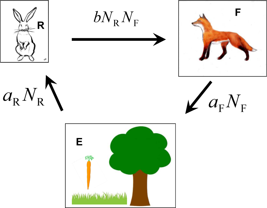
While the existence of intransitivity in competitive Lotka–Volterra models that generalise the original version for multiple species is well-known [34], the cyclic behaviour of the original version hints at possible intransitivity (according to our terminology, it can be called potentially intransitive). Here, we show that such intransitivity is indeed implicitly present in the original version of the Lotka–Volterra model [35,36], which is given by the following system
where NR represents the population of rabbits (R) and NF is the population of foxes (F). The model coefficients aR, aR, b and b′ are assumed to be positive indicating that the foxes win resources from the rabbits due to presence of the term bNRNF (b and b′ are generally different since NF and NR are measured in different resource units: in foxes and in rabbits). The intransitivity of this model is not apparent since this model does not explicitly mention the environment (E), but the presence of the environment is important. Indeed if NR = 1 and NF = 0 at t = 0, then NR → ∞ as t → ∞, which is physically impossible. In real life, this growth of rabbit population would be terminated by environmental restrictions: aR = aR(NE) → 0 and NE → 0 as NR → (NR)max. Here, NE represents free environmental resource, which is approximately treated as constant in the original Lotka-Volterra model. Figure 3 illustrates the intransitivity of this case: rabbits win from the environment, while foxes lose to the environment.
6. Fractional Ranking
Different options are often characterised by a set of criteria, say, indexed by α = 1, …, K. A ranking is then specified for each of these criteria r(α)(A). The notations which are used here are similar to those used in the previous sections. For example all of the following statements
indicate that B is preferred to A with respect to criterion α. The word fractional (or partial) is used to indicate that the comparison is performed only with respect to a single criterion: r(α) is a fractional ranking, ρ(α) is a fractional co-ranking, etc. (Another equivalent term is “partial”. This term is commonly used in calculus but this might be in conflict with “partial orders”, where “partial” is interpreted as “incomplete”—in partial orders, preferences are not necessarily defined for all pairs of elements). Of course, fractional ranking r(α) exists only if elements can be transitively ordered with respect to criterion α. No criterion alone determines the overall preference: for example, we might have r(1)(A) > r(1)(B) but r(2)(A) < r(2)(B). The fractional ranking can be either graded or sharp; the former can be called fractional utility. In this section, we deploy the results of the social choice theory, where different criteria represent judgment of different individuals.
6.1. Commensurable Fractional Rankings
When fractional rankings are graded they are interpreted as fractional utilities, i.e., they reflect the degrees of satisfaction with respect to specific criteria. It is reasonable to expect that these K degrees of satisfaction can be compared to each other; this means that the fractional utilities can be rescaled to be measured in the same common “units of satisfaction”. Hence, when different criteria are commensurable, absolute utility can be easily introduced according to equations
where the criterion weights w(α) are used to rescale units as needed. In principle, it is possible to consider cases when fractional utilities are combined in a non-linear manner but this would not change the main conclusion of this subsection:
Proposition 4 Commensurable fractional utilities correspond to an overall preference that can be expressed by the absolute utility r(…) and, hence, is transitive.
6.2. Commensurable Fractional Co-Rankings
There are two cases when utility must be replaced by co-ranking: (1) absolute fractional rankings do not exist or are unknown and (2) absolute fractional rankings exist but are incommensurable (That is we can compare the magnitudes of partial improvements, say, r(1)(A) − r(1)(B) and r(2)(A) − r(2)(B) but cannot compare the absolute magnitude, say, r(2)(A) and r(2)(A). This is a common situation since, as discussed in the next chapter, human preferences are inherently relativistic). The fractional preferences can always be expressed by fractional co-rankings, which are treated in this subsection as graded and commensurable. (The relative character of real-world preferences, which is reflected by co-rankings, is discussed further in the paper. The case of completely incomparable partial preferences is considered in the following subsection). The overall co-ranking is expressed in terms of the fractional co-rankings by the equation
where the weights w(α) represent the scaling coefficients, whose physical meaning is similar to that of the weights in Equation (48). Depending on the functional form of the fractional co-rankings, three cases are possible (1) fractional and overall co-rankings are transitive (in this case the fractional and overall utilities exist); (2) fractional co-rankings are transitive but the overall co-ranking is intransitive and (3) all co-rankings are intransitive. As discussed further in the paper, the second case is common when fractional co-rankings have non-linear functional forms, which can appear due to imperfect discrimination or for other reasons.
6.3. Incommensurable Fractional Preferences
In this subsection, the case of incommensurable fractional preferences is considered (irrespective of transitivity of fractional preferences). For example, it could be the case that ρ(1)(A,B) and ρ(2)(A,B) can not be rescaled to produce commensurable quantities. Grading of fractional rankings or co-rankings becomes useless if different gradings are incommensurable. The information that can be used in this case is limited to (1) sharp fractional ranking, if the fractional preferences are transitive or (2) indicator co-ranking (or sharp fractional co-ranking), if the fractional preferences are intransitive. The first case in considered first. If sharp (or incommensurable) fractional absolute rankings are strict, they represent an ordering as discussed in Section 2.2.
Arrow’s theorem [37] states that fractional orderings cannot be converted into overall ordering in a consistent manner. The conditions of being consistent are stipulated in the formulation of the theorem, which is given below and uses notations of the present work.
Theorem 1 (Arrow [37]) For more than two elements, a set of K fractional orderings cannot be universally converted into an overall ordering in a way that is:
- (a) Non-trivial (non-dictatorial): absolute ranking does not simply replicate one of the fractional rankings: r(…)≁ r(α)(…) for all α;
- (b) Pairwise independent: preference between any two elements does not depend on fractional rankings of the other elements, i.e., R(A,B) depends only on all R(α)(A,B), α = 1, …, K;
- (c) Pareto-efficient: A≻B when r(α)(A) > r(α)(B) for all α.
The underlying reason for the impossibility of Arrow-consistent conversion (i.e., complying with the three conditions of the Arrow’s theorem) of fractional-criteria orderings into overall ordering is intransitivity. This point is discussed further below with the use of the following proposition:
Proposition 5 Strict fractional preferences (represented by fractional rankings if transitive or by fractional co-rankings if intransitive) can always be converted into an overall strict preference in an Arrow-consistent way, which is (1) non-trivial (for K > 2), (2) pairwise independent and (3) Pareto-efficient.
The proof is straight-forward: the overall co-ranking defined by
is non-trivial, pairwise independent and Pareto-efficient. Indeed, (1) sign(ρ(A,B)) ≁ R(α)(A,B) for any α (we assume K > 2), (2) the formula for ρ(A,B) does not involve any characteristics of any third element (say C) and (3) ρ(A,B) = 1 when all R(α)(A,B) = 1. Here we put w(α) = 1 + ε(α), where ε(1), …, ε(K) are small random values, which ensure that ρ(A,B) = 0 only when A=B.
The existence of fractional rankings is not essential for this proposition and Equation (50) can be used when the fractional preferences are intransitive. If fractional co-rankings are transitive and fractional rankings exist, this, as shown below, cannot ensure transitivity of the overall co-ranking by Equation (50).
Proposition 6 Any Arrow-consistent conversion of fractional orderings into an overall strict preference is potentially intransitive.
Indeed, if the overall Arrow-consistent strict preference of Proposition 5 was necessarily transitive, this preference could be always converted into an Arrow-consistent ordering, which is impossible according to Arrow’s theorem. Here we refer only to potential intransitivity since the overall preference might be currently transitive under some specific conditions. For example, Pareto efficiency requires that A≻B≻C≺A when r(α)(A) > r(α)(B) > r(α)(C) for all α.
We conclude that intransitivity necessarily appears in overall preference rules that are consistently derived from a set of incommensurable fractional criteria. Despite intransitive co-ranking, the elements can still be transitively ordered by conditional ranking with respect to a selected reference set. This transitive ordering, however, is in conflict with the second condition of Arrow’s theorem (pairwise independence) due to dependence of conditional ranking on the reference set in intransitive systems (see Propositions 1, 2, B1 and B2). The conditions of Arrow theorem require that the overall preferences cannot have absolutely transitive co-rankings and, practically, violate at least one of the properties: transitivity or pairwise independence.
7. The Subscription Example
This section is dedicated to detailed analysis of the example “The Economist’s subscription” used by Dan Ariely [38] as an excellent demonstration of the relativity of human preferences: in the real world, we can express our preferences only in comparison with the other options available. Classic economic theory sees this kind of behaviour as irrational. While many examples from Ariely’s book “Predictably irrational” [38] are indeed linked to irrationality of human behaviour, relativity of our preferences in general and in choosing the The Economist’s subscription in particular is perfectly rational.
Sometimes we can make a choice in absolute terms without resorting to relative comparison. For example, considering The Economist’s subscription, I would reject an annual print subscription for The Economist priced at $1000 and agree to have this subscription for $10 without much thought or any further comparisons. One can see that these statements based on the perceived absolute values of the subscription and money are quite approximate and, probably, not suitable for the real world. Realistically, I do not know offhand whether I want The Economist print subscription priced at $120. To make this judgment, I need to estimate the value of money in terms of utility of published media and see if the offered price is reasonable or not. I would probably look at subscriptions for other magazines to make up my mind. In the end, I might decide that The Economist provides good value for the money, or that I can get a colourful magazine to read at much lower cost. My relative preference is perfectly rational; in fact, it would be irrational for me to make up my mind on the basis of the absolute value of money and the absolute utility of enjoying The Economist, without knowing the subscription market and undertaking relative comparisons.
7.1. Ariely’s Subscription Example
Consider the following options for subscription to The Economist
- (A) Web (W) subscription, $60;
- (B) Print & Web (P+W) subscription, $120;
- (C) Print (P) subscription, $120
The prices have been slightly adjusted from original $59 for W and $125 for P and P+W reported by Ariely [38] to make evaluation of this example more simple and transparent.
Ariely [38] determined that when only two options, A and B, are given, people tend to make their choices with the following frequencies:
However, when all three options are available, preferences become very different
Although option C is not chosen, it affects the choice between options A and B. While Ariely believes that this is irrational, we argue here that this is a perfectly rational choice conducted in line with a reasonable relativistic analysis of the offers. Note that the dependence of the choice on C cannot be explained within the conventional framework of absolute preferences (i.e., by any set of absolute utilities assigned to options A, B and C).
7.2. Evaluating Co-Rankings
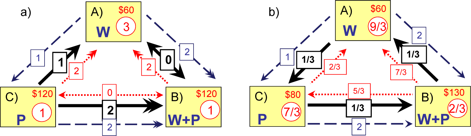
Since no additional information is given (for example, we have no idea about realistic costs of the options offered), the choice between the subscription options can be made rationally only on the basis of comparing these options to each other. We thus compare the options with respect to the two fractional criteria, prices p and values v, using three different grades: the same “∼” (ρ = 0), better “≻” (ρ = 1) and clearly better “≻≻” (ρ = 2). The following estimate of our relative preferences
seems reasonable. Note that the first relation is not a mistake: the symbol “≻” means “preferred to” and not “greater than”. Obviously, we prefer a lower price and p = $60 is clearly better than p = $120. Figure 4a shows that our assessment $60 ≻≻ $120 corresponds to the price utility
which can be evaluated from the equation
Higher utility corresponds to lower price and any price ≥ $150 is not seen as reasonable.
We concede that the print edition is more convenient than web edition P≻W (reading The Economist while sitting in an armchair and having a cup of coffee does have some advantage), although this convenience is not overwhelming. Having both print and web subscription is clearly better than any of these subscriptions alone. The result of comparison is shown in Figure 4a so that the overall co-ranking is given by
and
As specified by Equation (49), this co-ranking is obtained by summing fractional co-rankings ρ(v) and ρ(p) with equal weights and W = 2. When only two options, A and B, are available the conditional ranking with the reference set of
is given by
but when the choice is to be made by selecting from A, B and C, the conditional ranking using the reference set of
becomes
Here, we use Equation (11) with all weights gi set to unity. Hence, we would chose B from {A,B,C} but will have difficulty of selecting between A and B from {A,B}. (For the sake of our argument, it is sufficient to put ρ(A,B) = 0 and treat the preference between A and B as being close to 50% each. Ariely [38] indicates a marginal preference of A over B, which can be accommodated by introducing another grade of a preference—“marginally better” quantified by, say, 1/3 or 1/2. The co-ranking ρ(A,B) is thus redefined while the remaining co-rankings in Equation (56) are kept the without change. If 2ρ(A,B) = 1/3, then
since
and
. If 2ρ(A,B) = 1/2, then
since
. Here,
. The author has repeated Ariely’s experiment in class of 60 students with half of the class selecting between A and B, while the other half selecting between A, B and C. The results {85%, 15%} and {35%, 62%, 3%} clearly confirm the effect discovered by Ariely, although indicate a higher level of acceptance of electronic communications than a decade ago).
7.3. Potential Intransitivity of the Subscription Values
As suggested by Propositions 1, 2, B1 and B2, the dependence of the conditional rankings of A and B on the reference set
indicates potential intransitivity of our preference. This intransitivity is not clearly visible since our preferences Equation (57) do not form a strictly intransitive triplet, but current intransitivity may appear when conditions are altered. Here we consider a specific example, while a general case is treated in Appendix A. The subscription case shown in Figure 4a has a potentially intransitive value co-ranking and absolutely transitive price co-ranking. Indeed, current intransitivity can easily appear if we adjust the prices. Figure 4b indicate that the prices pA = $60, pB = $130 and pC = $80 correspond to the utilities of 3, 2/3 and 7/3 as specified by Equation (55). Our assessment of the subscription values remains the same as in Figure 4a. With the new price utilities, the overall co-ranking becomes
and our overall preferences given by
are currently intransitive as shown in Figure 4b.
If we need to get rid of intransitivity, the values of subscriptions have to be adjusted so that fractional utility r(v) can be introduced and then the overall utility r = r(v) + r(p) ensures transitivity of our preferences. Let r(v)(A) = 1, r(v)(B) = 3 and r(v)(C) = 2. This corresponds to replacing the last preference in Equation (53) by P+W≻P. This transitive correction does not necessarily represent human preferences better (in fact P+W≻P is not accurate for me, since I think that P+W is clearly better than P) but it removes potential intransitivity.
7.4. Discussion of the Choices
Our knowledge of the subscription market and, consequently, our analysis of the available options given above may be imperfect, but it is not irrational. It is based on a system of values and on a systematic comparison between these options—but why does our choice depend on the presence of option C? This seems to be illogical. We compare A and B and, with the information available to us, we have difficulties of making a choice between these options. Option C provides us with additional information that makes option B more attractive: the web subscription is given to us at no extra-cost, while the printed version of the magazine has a high cost and, presumably, high quality and high aesthetic value.
It can be argued that a buyer should care about the value of the product and the price but not about getting a good deal from a seller. This could be rational only if the buyer had a complete knowledge of the product and its future use. In the real world, a responsible buyer checks that he is getting a reasonable deal even if, in principle, he is prepared to pay more. A buyer who does not want a good deal is, in fact, irrational—in the real world, this buyer will be overcharged much too often.
An overzealous deal-seeker is, however, prone to manipulations and to buying goods and product features that he does not needed. Therefore, the fact that sellers can be manipulative should not be overlooked. The web subscription is given for free in option B because its web delivery has a very low cost. Perhaps, but there could be other reasons. For example let us assume that the realistic pricing of subscriptions is similar to the prices shown in Figure 4b. The subscription seller may then lift the price of pC from $80 to $130 to lure his customers into subscribing for option B. In this case the presence of C in the subscription list is not information but disinformation. How can the buyers protect themselves against such manipulations?
In transitive systems, preferences are absolute and independent of perspective. Proposition 1 and 2 show that, in intransitive systems, preferences depend on perspective: whether
or not depends on reference set
and on reference weights gi. Hence, a reasonable choice relies on a good selection of the perspective. Artificially or unscrupulously selected elements may distort the picture. In the subscription example, it might be desirable to weight the options by their estimated market shares. In this case the seller’s manipulations with option C would not have a significant effect on our choice.
Economic theory sees the inherent relativity of our preference as being irrational. While humans can make irrational choices at times, relative comparisons are very common and perfectly rational despite being inherently prone to intransitivity. In fact, in many cases relative comparisons are the only ones that are practically possible and avoiding them would be irrational. Enforcing transitivity does not necessarily make our assessments or theories more accurate but it does make our choices more stable, more immune from manipulations and easier to predict—transitive preferences are absolute and do not depend on third options. However, as demonstrated by Ariely’s subscription example, a real buyer in the real world is likely to have a (potentially) intransitive set of preferences.
8. Intransitivity Due to Imperfect Discrimination
Since it is often the case that exact values of the fractional utilities are not known or, maybe known but, to some extent ignored by decision-makers, we need to deal with approximate values of the parameters. This, as demonstrated below, leads to intransitivity.
8.1. Discrimination Threshold
In the real world, preferences are typically not revealed whenever difference in utility values are small, say, smaller than a given threshold ε. This corresponds to a coarse co-ranking ρ(α) defined by
The corresponding coarsened fractional equivalence is understood as
Fractional co-rankings determine the overall preference according to Equation (6). Despite the existence of commensurable fractional utilities and the overall utility Equation (48) for the fine preference (i.e., original preference with perfect discrimination), the coarse preference specified by Equation (62) is intransitive and does not have an overall utility (Coarsening of partial co-rankings corresponds to coarsening partial preferences, understood according to coarsening of preferences as defined in Appendix B. The overall preferences, however, do not represent coarsening of the original (fine) overall preferences, at least because the former can be intransitive while the latter are transitive). The intransitive properties of coarsening are characterised by the following proposition due to Yew-Kwang Ng [39].
Proposition 7 (Ng [39]) The overall preferences that correspond to threshold coarsening of K independent fractional utilities are
- (a) weakly intransitive (existence of A∼B∼C≻A) if K = 1,
- (b) semi-weakly intransitive (existence of A≻B∼C≻A) if K = 2 and w(1)ε(1) = w(2)ε(2),
- (c) strictly intransitive (existence of A≻B≻C≻A) if K = 2 and w(1)ε(1) ≠ w(2)ε(2) or K ≥ 3.
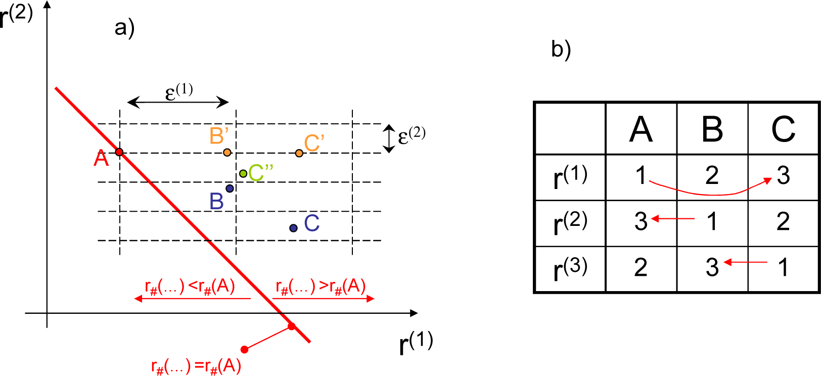
The details of the definitions characterising intransitivity can be found in Appendix E. The proof is illustrated by Figure 5. The case A∼B′∼C′≻A can be found in Figure 5a (the second coordinate, r(2), can be ignored in this case). The semi-weakly intransitive triplet A≻B∼C″~A in the same figure does not depend on the direction of the red line of constant fine utility. Finally, the points A≻B≻C≻A form a strictly intransitive triplet (note that C must be above the red line). In the three-dimensional case shown in Figure 5b, we select ε(α) = 1.5, α = 1, 2, 3, hence 1∼(α) 2∼(α) 3≻(α) 1. Most values in the table are equivalent, while the three strict preferences of 3 over 1 are shown by the arrows. It is easy to see that the listed points form a strictly intransitive triplet A≻B≻C≻A.
Practically, coarsening in multidimensional cases becomes strictly intransitive. The cases without strict intransitivity are degenerate: either dimensions are redundant or coarsening is performed after merging the fractional variables into the overall utility (instead of independent coarsening for all or some of the criteria). From a philosophical perspective, this statement can be presented as a continuum argument for intransitivity [20]: small alterations are commonly overlooked for secondary parameters but can be accumulated into critical differences.
8.2. Imperfect Discrimination Due to the Presence of Noise
If the exact value of utility r is not known (which is often the case in the real life), this can be expressed by adding a random variable ξ, which is assumed to be Gaussian, to the utility
The value y is a measured, perceived or known estimate of the unknown value r. When comparing A and B we need to estimate Δr = r(A)−r(B) from known Δy = y(A)−y(B). We can write Δy = Δr+ξ, where a difference of two independent Gaussian random values is shown as a Gaussian random value, ξ. While obviously Δr = 〈Δy〉, averages cannot be evaluated from a single measurement—the preference must be evaluated deterministically on the basis of known value Δy. It is clear that small changes of Δy should be ignored (i.e., Δr ≈ 0) since |Δy| ≪ σ is likely to be induced by the random noise ξ. In this case the sign of Δy does not tell us much about the sign of Δr. If, however, |Δy| ≫ σ, then Δr ≈ Δy with a high degree of certainty so that Δy and Δr are most likely to have the same sign. The magnitude σ of the noise is presumed to be known. While coarsening Equation (62) implements these ideas abruptly (all or nothing), it is clear that our confidence in estimating r increases gradually as y increases.
The estimate Δy of the value Δr is considered to be satisfactory if
with a sufficiently small β. In this case our preference is modelled with the use of the following function
This function, which is illustrated in Figure 6, coincides with graded co-ranking Δr = r(A) − r(B) when our estimate is satisfactory and is set to zero otherwise, i.e., unsatisfactory estimates are ignored. The average of this function is
where ε = 21/2σ/β. The function
represents Δy multiplied by a factor representing reliability of Δy giving a satisfactory estimate for Δr, i.e.,
is the reliable fraction of Δy. This models our inclination to ignore small Δy = y(A) − y(B) and accept large Δy while comparing A and B.
Assuming that the measured values y(α) of the fractional utilities r(α) are different from the true values due to presence of some random noise, we are now compelled to define the fractional co-ranking by
where
, is the fine-graded co-ranking, which does not take into account the presence of the noise (i.e., is based upon Δr = Δy), and ε(α) is determined by the intensity of noise in direction α. The fine co-ranking and two coarse co-rankings that correspond to threshold coarsening Equation (62) and Gaussian coarsening Equation (67) with ε(α) = 1 are shown in Figure 7a. The effect of smooth coarse grading on intransitivity is qualitatively similar to the threshold case:
Proposition 8 Gaussian coarsening in multiple dimensions K > 1 leads to strict intransitivity provided that not all w(α)ε(α) are the same.
Figure 7b demonstrates intransitivity A≻B≻C≻A for the case when coarsening occurs along the first direction (that is ε(1) = 1 and ε(2) = 1/10).
9. Risks and Benefits
The problem considered in this section has two main parameters that represent different quantities and are not trivially combinable into a single value. One of these parameters has a greater uncertainty or is contaminated by random noise. While this consideration is generic, we interpret these parameters as risk and benefit. This is determined by three factors. First, as discussed in the introduction, balancing risk and benefit has been investigated in various contexts (decision-making under uncertainty, personal preferences, portfolio management, etc.). Second, risk and benefit are not commensurable (at least not in a trivial or obvious manner). The benefit is defined as the average pay-off so that increasing or decreasing risk does not affect it directly. Given the benefit (which is presumed to always have a positive utility), in real life people can be risk-adverse or risk-seeking depending on the situation but, in this work, we treat risk as a detrimental factor having negative utility. Third, benefits (which are linked to mean values) are typically known with less uncertainty than the associated risks (which are linked to stochastic variances).
The fact that people tend to ignore small increments in risk has been noticed in many publications. (Here we refer only to small increments of risk—most people are over-sensitive to small risks in comparison to absence of any risk. Typically people are risk-seeking for small probabilities of gains and substantial probability of losses but the same people are risk-aversive for small probabilities of losses and substantial probability of gains [40]). Rubinstein [19] suggested that the Allais paradox is linked to common treatment of close probabilities as being equivalent and noted that intransitivities are likely to appear in this case, undermining the existence of utility. Leland [41] noted limited abilities of individuals to discriminate close probabilities. Lorentziadis [42] introduced division of probabilities into ranges to reflect coarsened treatment of probabilities. This approach requires an individual to discriminate very close probabilities located of different sides of the range divides (this does not seem realistic but preserves transitivity). Here, we follow these works and assume that the risk is known to us with a substantial degree of uncertainty.
9.1. Hidden Degradation
It is often the case that seemingly positive incremental developments are accumulated to create problems or malfunctions. This is impossible in transitive systems (due to the absolute nature of transitive improvements) but, if intransitivity is present, then an obvious improvement in one parameter (e.g., higher benefit) may be accompanied by a tacit decrease in performance with respect to another parameter (e.g., increasing risk). The problem occurs when the risk becomes too high and the system malfunctions or collapses. Tacit loss of competitiveness is called hidden degradation. In general, evolution of an intransitive system may result in competitive escalation or competitive degradation. The degradation can be explicit or hidden [5–7].
Consider the following example: in order to improve the performance of industrial turbines, the manufacturers commonly cut technical margins for operational conditions of the components. This does not make the turbines unsafe and does improve their efficiency. Competition between manufacturers forces each of the competitors to cut margins further and further to reach higher and higher efficiency producing turbines that become more and more sensitive to fuel, servicing and other requirements. As discussed above, we immediately acknowledge the increase in performance but hardly notice any tiny increments in risk associated with reducing the margins. However, these increments can gradually accumulate into vulnerability of the product. An unexpected change in conditions (which can be very small in magnitude—a different fuel, for example) can cause a malfunction or even make the technology impractical. In intransitive conditions, competition and gradual apparent improvements may result in a collapse due to accumulated negative effects, which are collectively referred to as “risk”. This is intransitivity in action: each new design is better than the previous one and, yet, one day the latest and seemingly best design fails miserably and gives way to alternative technology.
It is interesting that knowledge of the treacherous nature of intransitive competition does not always allow us to avoid its unwanted consequences. For example a cautious turbine manufacturer deciding not to improve the efficiency of its turbine is likely to be forced out of business well before any intransitive effects will come into play.
Similar effects can be found in biology, economics and other disciplines. For example, as the capacity for economic growth becomes more and more saturated, investors have to undertake higher and higher risks to uphold their profits. Accumulation of invisible risks makes the market unstable, and, one day, the market collapses. There might be an external factor that triggers the collapse, but the fundamental reason that makes this collapse possible is the intransitivity of economic competition.
9.2. Competitive Simulations for Risk-Benefit Dilemma
This dilemma has two independent variables: (undesirable) risk y(1) and (desirable) benefit y(2). In a simple transitive model, there exists a 1:1 trade off between the risk and the benefit according to co-ranking defined by
It is obvious that, due to its linear form, co-ranking Equation (68) implies the absolute utility, which can be written as
Existence of the absolute utility r0(A) indicates the transitivity of this case.
If there is some uncertainty in evaluating the risk, the co-ranking takes another form in accordance with Equation (67)
with ε = 1 and k = 1. Here we put k = 1 but, in principle, k can be set to other values, thus changing the degree of coarsening. If k = 0, then Equation (70) coincides with Equation (68). If k > 0, than the co-ranking becomes intransitive and the corresponding absolute utility does not exist.
In the simulations, the competing elements are represented by particles (the same as particles used in modelling of reacting flows). The particles compete according to the preferences specified by the co-ranking functions. The losers are assigned the properties of the winners subject to mutations, which are predominately directed towards y(1) = y(2) = 0. The details can be found in previous publications [5–7,43]. The gray area in Figure 8 indicates prohibited space. The boundary is Pareto-efficient: it is impossible to increase the benefit without increasing the associated risk.
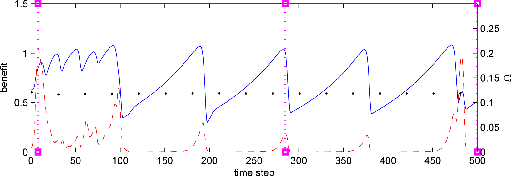
The simulations are qualitatively similar to previous simulations [7,43] with a power-law representation of the co-ranking functions. The simulations start from arbitrary conditions but promptly (within ∼20 time steps) relax to quasi-equilibrium states that may continue to evolve. These initial evolutions are similar in transitive and intransitive cases and, as shown in [7], these cases have similar quasi-equilibrium distributions (although the present simulations show more variations). The transitive cases Equation (68) quickly reach equilibrium and stay in the equilibrium forever. The intransitive cases Equation (70) continue to evolve cyclically: the benefit and risk grow until the system collapses into a defensive state of low benefit and low risk. Figure 9 indicates the existence of two periods of around 100 steps and 30 steps respectively in intransitive simulations with co-ranking defined by Equation (70). There is a switch to the dominant mode at 100 steps. The dots indicate the equilibrium state, which is necessarily achieved in transitive simulations with co-ranking defined by Equation (68). The dashed lines in Figures 9 and 10 demonstrate the apparent similarity of intransitive simulations to a transitive preference (although not given by Equation (68)). This similarity disappears prior to collapses of the high-benefit states of the system. The details are given in Appendix D.
10. Thermodynamics and Intransitivity
Physical thermodynamics is fundamentally transitive due to restrictions imposed by the second and zeroth laws. For example, TA > TB and TB > TC require that TA > TC. The concept of negative temperatures is compliant with the laws of thermodynamics and does not alter transitivity. Negative temperatures are placed above positive temperatures (for example T = −300 K is hotter than T = 300 K) but all temperatures are still linearly ordered according to −1/T. That is T = +0 K is the lowest possible temperature, while T = −0 K is the highest possible temperature (see [44]). If +0 K were identical to −0 K (which is not the case), then the thermodynamic temperatures would be intransitive). Hence, the constraints of physical thermodynamics allow for cyclic or intransitive behaviour only in thermodynamically open systems. There is no evidence of any kind that the laws of thermodynamics are violated in complex evolutionary processes (biological or social). Increase of order in a system is always compensated by dispersing much larger quantities of entropy. The question that is often discussed in relevant publications [45] is not the letter but the spirit of the thermodynamic laws—the possibility of explaining complex evolutions using thermodynamic principles. Such explanations can be referred to as apparent thermodynamics (i.e., thermodynamics-like behaviour explained with the use of the theoretical machinery of thermodynamics).
10.1. Transitive Competitive Thermodynamics
As noted above, complex evolutionary systems are closer to thermodynamic systems placed in an environment than to isolated thermodynamic systems. The latter are characterised by maximisation of entropy while the former are characterised by minimisation of Gibbs free energy or by maximisation of free entropy, which, effectively, is Gibbs free energy taken with the negative sign. Typical free energy and free entropy have two terms: configurational and potential. In competitive systems, the configurational terms reflect existence of chaotic mutations, while the potential terms reflect the ordered competitiveness (or fitness, or utility), which represents the propensity of elements to survive (theory and examples can be found in previous publications [5–7]). Here we refer to effective potentials that reflect competitiveness of elements placed into certain conditions (or environment). As in conventional thermodynamics, equilibrium is the balance between chaos (configurational terms) and order (potential terms). This approach explains transitive effects such as evolution directed towards increase of fitness, which is characterised by increase in apparent entropy. The process of competition is also characterised by production of physical entropy at least because information is continuously destroyed when the properties of losers are discarded.
While physical thermodynamics is always transitive, the same cannot be stated a priori about apparent thermodynamics.
10.2. Nearly Transitive Systems
Here we refer to the systems as intransitive but their evolution remains close, in one way or another, to evolution of transitive systems. These cases are shown in Figure 11 as: (a) locally intransitive systems, where large-scale preference is transitive or (b) globally intransitive systems, where transitivity is preserved locally. In case (a), we can treat evolution as transitive if local details of the evolution can be neglected. In this approximate consideration, we treat elements A1 B1 and C1 as equivalent and distinguish only transitive preferences
This corresponds to the transitive closure of the original preference [5].
In case (b), the properties of conventional thermodynamics are preserved as long as our consideration is confined to regions where conditions are transitive, but intransitive cycles can appear on larger scales. Consider competitive system shown in Figure 11b where the competition between A, A1, …,A3 is transitive and unique ranking is possible within the region around element A. Under conditions specified in [5], this local competition can be characterised by competitive potentials χ, which are analogous to chemical potentials of conventional thermodynamics taken with a negative sign. However, the competition is intransitive if we look at larger scales: A≺B≺C≺A. If three identical systems have elements A, B and C as leading particles, the competitive potentials are related to each other by
Note that we cannot write χA < χB < χC < χA since this does not make mathematical sense. Competitive potentials are numbers in transitive systems but they must be treated as more complex objects in intransitive systems.
10.3. Strong Intransitivity
If strictly intransitive triplets are both local (or dense—can be found in any small vicinity of every point) and global, we identify this intransitivity as strong. The properties of such systems differ from properties of conventional thermodynamic systems, and the benefits of using thermodynamical analogy for stochastic theories of strongly intransitive systems are not clear [5,6]. In these systems, the similarity with conventional thermodynamics becomes quite remote and the term “kinetics” seems to be more suitable.
Complex kinetics of strongly intransitive competitive systems must at least account for
- rapid relaxation to a quasi-steady state (which, possibly, can be approximately treated as transitive) with subsequent slow evolution;
- the possibility of alternative directions of evolution (i.e., competitive degradation or competitive escalation);
- violation of Boltzmann’s Stosszahlansatz (the hypothesis of stochastic independence of the system elements) and formation of cooperative structures.
11. Discussion and Conclusions
This work endeavours to introduce a consistent approach to treat the problem of intransitivity, which is relevant to many different fields of knowledge that have to deal with preferences and/or competition. In general, a theoretical treatment of competition and preferences allows for two alternative self-consistent frameworks: absolute and relativistic. The first framework presupposes the existence of absolute characteristics that are commensurable and known exactly. This framework is fundamentally transitive and more simple from the perspective of theoretical analysis. The second framework is based on relative characteristics. In this framework, assessment of performance of the elements depends on perspective and intransitivity is common. Many real world effects that cannot be explained within the absolute framework (and thus are commonly viewed as irrational or abnormal), become perfectly logical in the relativistic framework.
The focus of this work is the existence of key links between intransitivity and dependence of conditional preferences on the reference group. Our main conclusion is that intransitivity must be typical for systems involving preferences and competition since intransitivity appears under any of the following conditions, all of which are common in the real world:
- ♦ relative comparison criteria or
- ♦ multiple comparison criteria that are incommensurable or
- ♦ multiple comparison criteria that are known approximately or
- ♦ comparisons of groups of comparable elements.
In some disciplines (e.g., social choice, population ecology), intransitivities have been acknowledged and studied but in other disciplines (law, economics) they tend to be ignored. While intransitivity represents rather special cases in law that legal professionals need to be aware of, intransitive behaviours seem to be ubiquitously present in economic systems. This does not mean, of course, that assumptions of transitivity are always erroneous, but large economic systems tend to behave in a typically intransitive manner (e.g., with cycles and collapses). It is difficult to say if intransitivity of personal preferences is the main factor causing this behaviour (There could be other reasons. For example, intransitivity of competition, which is not related to intransitivity of personal preferences of the consumers, has been detected in the American car industry [43]). It is worthwhile to note that intransitive systems can behave so that their short-term evolution seems perfectly transitive—this effect corresponds to transitive theories. This point is well illustrated by the competitive simulations of the risk/benefit dilemma: segments of this evolution seem to be transitive, until a point is reached where the system collapses and then behaves cyclically, which is typical of intransitive competitions and impossible in transitive competitions. Therefore the main purpose of this work is not in criticising assumptions of transitivity, which can be quite reasonable in many circumstances, but in pointing out that these assumptions are excessively restrictive to deal with more complex phenomena. We have all indications that emergence of complexity in competitive systems is linked to intransitivity. Disciplines that dismiss intransitivity outright as being “irrational” or “non-scientific” are likely to experience an increasing pressure of a paradigm shift in coming years.
Transitive systems are characterised by absolute quantities (e.g., absolute rankings). Absolute quantities do not exist in intransitive systems, which have to operate with relative quantities, such as co-rankings. Thermodynamics (here we refer to both physical thermodynamics and thermodynamics-like theories) is primarily equipped to deal with transitive phenomena and the physical thermodynamics is fundamentally transitive. Although apparent thermodynamics may allow for a limited presence of intransitivity, it seems that the strongly intransitive effects should be studied by the relevant complex kinetics, which is at the very beginning of its development. The main question is whether common features observed in a number of complex systems of different physical nature can be analysed at a generic level while neglecting less significant case-specific details. The author of this work believes that the answer to this difficult question is positive and that it requires consideration of evolving systems with competition based on generally intransitive preferences. The following patterns of behaviour are indicative of presence of intransitivity in competitive systems:
- relativity of strength and dependence of preference on perspective
- cyclic behaviour instead of relaxation to a unique equilibrium
- relatively slow evolutions punctuated by sudden collapses and changes
- complex patterns of behaviour (e.g., cooperative structures).
It must be noted that there exist psychological barriers in accepting intransitivity as a realistic phenomenon, at least in some fields. This has delayed investigation of complex effects, although reasons for this are understandable. The transitive world is black and white: fit versus unfit, strong versus weak and good versus bad—this is a simplification that can be useful as it is more easily amenable to theoretical analysis or explanation. The intransitive world is much more colourful: what is good or bad depends on perspective and on the current situation, and possible situations have endless varieties. While theoretical advances are more difficult in intransitive systems, there lays the explanation of the complexities of the real world.
Acknowledgments
The author thanks D.A. Klimenko for many fruitful discussions and a number of useful corrections. The author acknowledges funding by the Australian Research Council.
Conflicts of Interest
The author declares no conflict of interest.
Appendix
A. Potential Intransitivity
It is possible to have a potentially intransitive co-ranking ρ(…, …) that defines a transitive preference on a given set of elements but cannot be represented by transitive relation Equation (10). In this case there always exists an absolutely transitive co-ranking that defines an equivalent preferences on this set. Indeed, transitivity of the preference allows for the introduction of an absolute ranking and then the transitive co-ranking is determined by Equation (10). While co-rankings that cannot be represented by Equation (10) may define a transitive preference on the current set of elements (current transitivity), the underlying rules for these preferences can be expected to be intransitive and intransitivity can be revealed when these co-rankings are used in a different context or conditions. This is illustrated by the following example.
Consider a transitive fractional preference between a set three elements
which corresponds to the co-ranking
If δ = 0 in the relation
where
is absolutely transitive approximation for ρ(1)(C,A), then fractional co-ranking Equation (A2) can be represented by Equation (10) in terms of the following absolute fractional ranking
However, if δ1 ≠ 0, this representation is impossible. In this case setting ρ(1)(C,A) ≥ 0 to
and ensuring that δ1 = 0 would remove potential intransitivity but alter the magnitude of our preference. Note that a triplet Equation (A1) with δ1 ≠ 0 can always be found in an arbitrary set with a potentially intransitive co-ranking (otherwise we may define r(B) = r(A) + ρ(B,A) for fixed A and arbitrary B).
While intransitivity is not currently visible in this example, it can appear when co-ranking Equation (A2) is used in a different way. The preference Equation (A1) does not have any rules specified for other elements, but we can investigate how this preference is combined with other fractional preferences that are strictly transitive. Consider a fractional ranking for the second criterion defined by
This ranking corresponds to the fractional co-ranking
If the overall co-ranking is defined as the average ρ = (ρ(1) + ρ(2))/2 then we obtain
If δ1 > 0, then selecting δ1/2 > ϵ> 0 determines an overall preference that is currently intransitive.
The case δ1 < 0 is treated in a similar manner. If δ1 = 0, intransitivity cannot appear. This discussion can alternatively be summarised in form of a short proposition:
Proposition A1 A potentially intransitive co-ranking can always be represented as a superposition of a currently intransitive co-ranking and an absolutely transitive co-ranking.
Three elements with original co-ranking ρ0, where ρ0 = ρ(1) in Equation (A3) with δ1 ≠ 0, can always be selected from a set with potentially intransitive co-rankings. Consider ρ0 = ρ1 + ρ2 where, ρ1 = −ρ(2) defined by Equation (A7) is transitive, and ρ2 = 2ρ specified by Equation (A8) is currently intransitive with a proper choice of ε. This decomposition is extended to the remaining elements so that ρ1 remains absolutely transitive. The representation ρ0 = ρ1 + ρ2 is, obviously, not unique.
B. Preference Properties and Indicator Co-Ranking
B.1. Coarsenings and Refinements
Consider two different preference rules specified on the same set of particles: ≺a and ≺b. Rule b represents a coarsening of rule a if A≺bB demands that A≺aB for any A and B (although A∼bB may correspond to any of A∼aB, A≺aB or A≻aB). If rule b represents a coarsening of rule a then the same property is expressed by saying that rule a represents a refinement of rule b, implying that A⪯aB demands that A⪯bB for any A and B (if A≻bB was correct, then this would demand A≻aB and thus contradict A⪯aB). (Statement “relation ⪯b contains relation ⪯a” is another equivalent, which is often used in literature but can be confusing in the context of the present work). If rules a and b are refinements of one another, then these rules are obviously equivalent.
B.2. Transitive Preferences in Intransitive Systems
The transitive closure of a preference (generally intransitive) is the minimal (i.e., most refined) transitive ordering that represents a coarsening of the original preference (see the Appendix in [5] for details). The ordering produced by the transitive closure is indicated by the subscript “t” (i.e., ≺t, ∼t, ⪯t, etc.) or by ≺≺, which is equivalent to ≺t, and by ≈, which is equivalent to ∼t. Hence the relation A≺≺B, which is expressed as “A is transitively preferred to B”, indicates that A≺B and A≺tB (where preference ≺ is generally intransitive). The relation A≺≺B implies that there should not exist any set {C1,…,Ck} such that A≺B⪯C1⪯…⪯Ck⪯A and, in particular, there is no such C that can form an intransitive triplet C⪯A≺B⪯C.
The symbol ≼, which is used to indicate ≺ but not ≺≺, should be distinguished from ⪯, which implies ≺ or ∼. In general, comparison of A and B belongs to one of the five mutually exclusive possibilities listed in the second row of the following table
![Entropy 17 04364f16]()
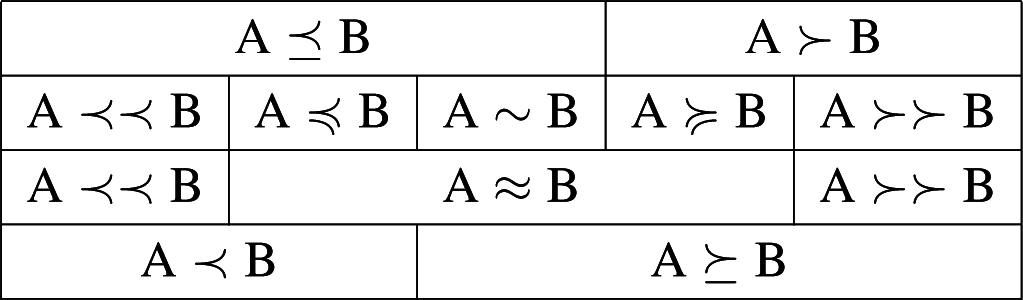
B.3. Transitivity and the Indicator Co-Ranking
Different versions of Propositions 1 and 2 are formulated below for conditional indicator rankings, i.e., for
defined by Equation (24)—the average conditional rankings based on the indicator co-ranking R(A,B).
Proposition B1 If the underlying preference is currently transitive, then the preference induced by the conditional indicator ranking (i.e.,
represents a coarsening of the underlying preference for any reference group.
Demonstrating the validity of this statement is not difficult. Due to transitivity, the preference A⪯B demands that R(A,C) ≤ R(B,C) for any C. Note that A≺B but R(A,C) = R(B,C) is possible for some C. We compare definitions of
and
by Equation (24) and conclude that A⪯B demands
, since R(A,Ci) ≤ R(B,Ci) for all Ci ∈
. Note that the combination of
and A≺B is possible for some
.
Proposition B2 If conditional indicator rankings based on different reference groups are strictly nonequivalent (i.e., there exist at least two elements A and B and at least two groups and so that and, then the underlying preference is currently intransitive.
Indeed, if the underlying preference were currently transitive, then, according to Proposition B1, preferences induced by the conditional indicator ranking would be coarsenings of the underlying preference. Therefore,
demands A≺B and
demands A≻B, which are contradictory. Hence the underlying preference must be intransitive.
If an underlying preference is defined for the elements, any two groups of elements
and
can be compared on the basis of the group indicator co-ranking defined by Equation (25), that is
iff
. We note that
Proposition B3 Group preference based on the indicator co-ranking is not necessarily transitive even if the underlying element preference is currently transitive.
Consider three sets
,
and
, where the numbers indicate the absolute rankings of nine distinct elements. It is easy to see that
since
. This example corresponds to the dice shown in Figure 1b.
C. Primary and Secondary Rankings
This appendix presents definitions and statements related to the indicator co-ranking R(…, …) that are intended for characterisation of the level of intransitivity in large and, possibly, evolving systems. The main assumption of this section is that all elements in system
are connected and form an overall group
, implying that there is a positive weight gi = g(Ci) > 0 specified for every element Ci ∈
. In this section, weights gi are associated with the whole system
and thus is the same for all groups
, which are referred to in this section as sets
, q = 1, 2, … to emphasise that the element weights are specified only for the whole system.
C.1. Current Rankings
Consider a system
of connected elements. The current ranking is defined by
that is R*(A) is the conditional ranking Equation (24) of element A with respect to all other elements in the system. In the same way the current ranking can be introduced for an arbitrary set
where G0 and Gq are total weights of the system and of the set
. The group co-ranking
is introduced according to Equation (25). The current ranking R*(…), the underlying preference ≺, and the corresponding indicator co-ranking R(A,C) are referred to as primary when we need to distinguish them from secondary characteristics.
The preference induced by the primary current co-ranking is referred to as secondary as it is now considered as the underlying preference for the secondary characteristics. The secondary current ranking is defined analogously to the primary current ranking
but with the use of the secondary co-ranking function R″ (A,B), which is introduced on the basis of the secondary preference (denoted by ≺″) and determined by the primary current ranking:
C.2. Properties of Current Rankings
The current ranking is a special case of conditional indicator-ranking, i.e., R*(A) is
with set
expanded to the whole system
. The following propositions characterise properties of
Proposition C1 If the primary preference is currently transitive, the secondary preference is equivalent to the primary preference: for any A and B.
The proof is similar to the proof of Proposition B1, but the case of R*(A) = R*(B) (i.e., A∼″B) is now impossible when A≺B. Indeed, all elements are presumed to be connected and present in the reference set in definition of the current ranking. Hence, the terms R(A,B) = −R(B,A) < 0 are present in the sums Equation (C1) evaluated for R*(A) while including Ci =B, and R*(B) while including Ci =A.
Proposition C2 If B is transitively preferred to A in a generally intransitive preference, then the preference of B over A is preserved by the current ranking: A≺≺B =⇒ R*(A) < R*(B) ⇔A≺″B
Although this proposition refers to a transitive preference A≺≺B in a preference ≺ that is generally intransitive and is thus different from the previous statements, its proof is similar. The relation A≺≺B requires that A≺B and there are no Ci that satisfies Ci A≺B Ci. Hence, R(A,Ci) ≤ R(B,Ci) and R(A,B) = −R(B,A) < 0 so that R*(A) < R*(B) as defined by Equation (C1). Note that the inverse statements R*(A) < R*(B) =⇒ A≺≺B and R*(A) < R*(B) =⇒ A≺B are incorrect in intransitive systems.
Since the preference specified by the primary current ranking is transitive, the preferences specified by the primary and secondary current rankings must be equivalent according to Proposition C1:
Here, Proposition C1 is applied to secondary (as primary) and tertiary (as secondary) preferences. The conclusion is that there is no independent tertiary preferences as they coincide with the secondary preferences. Equivalence of the primary and secondary rankings, however, does not imply that these rankings are identical: generally R*(A) ≠ R**(A). Deviations of secondary ranking from primary ranking indicate intransitivity in evolutions of competitive systems as determined by the following theorem:
Theorem C1 The following statements are correct for a system of connected elements (i.e., g(Ci) > 0 for any Ci ∈
):
- (a) If the primary preference is currently transitive, the primary and secondary current rankings coincide (i.e., R*(Ci) = R**(Ci) for all Ci ∈ ).
- (b) If the primary and secondary rankings coincide (i.e., R*(Ci) = R**(Ci) for all elements Ci ∈ ), then the secondary preference is a coarsening of the primary preference (i.e., Ci ≺″Cj =⇒ Ci ≺Cj).
- (c) In particular, if the primary and secondary rankings coincide and are strict (i.e., current rankings of different elements are different: R*(Ci) ≠ R*(Ci) for any Ci ≁ Cj), then the primary preference is currently transitive.
Proof. Statement (a) immediately follows from the equivalence of primary and secondary preferences, as stated in Proposition C1, while statements (b) and (c) require detailed consideration.
Let us sort all elements into k sets of decreasing primary ranking
; i.e., qth set
contains nq ≥ 1 elements that have primary current ranking
. The elements C1, …,Ci, …,Cn are thus ordered according to decreasing primary ranking. Figure C1 shows the structure of the n × n matrices Rij = R(Ci,Cj) and
, which correspond to the primary and secondary co-rankings. The co-ranking of different sets is denoted by
for primary preferences and by
for the secondary preferences. The average primary current ranking of a set is denoted by
, while the average secondary current ranking is denoted by
. These quantities are specified by Equations (24), (25) and (C1)–(C4). Obviously
for all q due to equivalence of the primary and secondary current rankings as stated in the theorem (i.e., R*(Ci)= R**(Ci) for all Ci ∈
).
Figure C1.
Co-ranking matrix with elements ordered according to their current rankings.
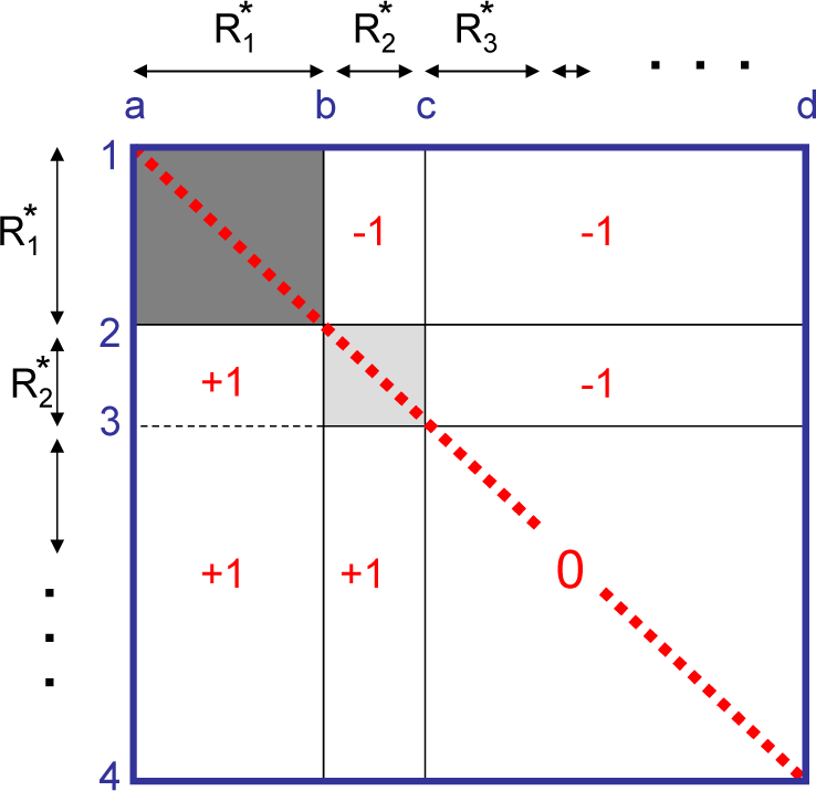
The first (leading) set
is considered first. The co-rankings
and
, which are determined by the sums over the dark square region a1-b1-b2-a2 (Figure C1), are zeros as the matrices Rij and
are antisymmetric. Since
is the same as
while
, the co-rankings
and
evaluated in terms the corresponding sums over the rectangle a2-b2-b4-a4 must be the same. Hence Rij = 1 in this rectangle since in any other case the sums
cannot coincide with
.
Since the co-ranking matrices are antisymmetric, Rij = −1 and
in the rectangle b1-c1-c2-b2. We take into account that
(the sums over the dark squares are zeros) and reiterate our previous consideration for rectangle b3-c3-c4-b4, where
and the sums
and
must be the same. Hence, Rij = 1 in this rectangle. Continuing this consideration for the remaining sets q = 3, 4…, k proves that
provided i and j belong to different sets.
If i and j belong to the same set, then
according to Equation (C5) and either Rij = 0 or competition is intransitive within the set (if the primary preferences within the set q were transitive then, according to Proposition C2, Ci≻Cj demands R*(Ci) > R*(Cj), which contradicts Ci,Cj ∈
). The secondary preference represents a coarsening of the primary preference since Rij00 > 0 demands Rij > 0 (when j and i belong to different sets), while
may correspond to Rij > 0, Rij = 0 or Rij < 0 (when j and i belong to a common set).
If current rankings of all elements are different, that is all nq = 1 for all q, then
since all i ≠ j always belong to different sets. This means that the primary preference coincides with the secondary preference based on primary current ranking and is transitive. ■
C.3. Maps of Current Rankings
The statements proven in the previous subsection suggest a relatively simple method of analysing intransitivity in large systems. This method, which is based on ranking maps (i.e., plots of primary current ranking R* of the elements against their secondary current ranking R**), indicates the presence, intensity, extent and localisation of intransitivity by deviations from the line R* = R**. We wish to stay under the conditions of Theorem C1(c), and avoid complexities related to statement b of this theorem since, in this case, equivalence between the primary and secondary rankings ensures transitivity. However, in the case of g(Ci) = 1, which perhaps is most common in practice, coincidences of primary rankings for different elements R*(Ci) = R*(Cj) for i ≠ j are likely due to the limited number of values spaced by 1/n that these rankings can take. The practical solution for this problems is simple—consider g(Ci) = (1 + εi)g0(Ci), where εi represent small random values and g0(Ci) are the original weights. Presence of these small values does not significantly alter the maps but makes coincidences R*(Ci) = R*(Cj) impossible unless all properties of the elements Ci and Cj are identical, which is sufficient for our purposes.
Two (or more) sets (or groups) are said to be subject to a preference when all possible selections of elements from these sets are compliant with the preference. For example
implies that sets
and
are subject to preference ≻≻ so that Ci(q) ≻≻Cj(p) for any Ci(q) ∈
and any Cj(p) ∈
. According to these notations, the index i(q) runs over all elements of set
. In this subsection, we consider partition of all elements in the system into range sets, where each set is represented by a range of primary current ranking (and consequently by a range of the secondary current ranking). The range sets are non-overlapping and jointly cover all elements.
We now turn to consideration of the R* versus R** maps. Consider an intransitive preference and its transitive closure. In this closure, the elements C1, …,Cn are divided into k transitively ordered sets
of elements that are transitively equivalent within each set. That is for any Ci(q) ∈
and any Cj(p) ∈
Proposition C2 indicates that R*(Ci(q)) > R*(Cj(p)) and R**(Ci(q)) > R**(Cj(p)) when q < p, that is the ranges of current rankings of different sets do not overlap. Hence sets
represent a set of range sets. This implies equivalence of primary and secondary set co-rankings
for all p and q. Note that
for any q. This also implies that
for any q. The property expressed by Equation (C9) is reflected in the following proposition
Proposition C3 The primary and secondary average current rankings of range sets coincide if and only if these sets are subject to a transitive primary preference (although this preference may remain intransitive within each set).
First we note that current primary set rankings of different range sets cannot coincide. The rest of the proof is similar to that of Theorem C1, where the leading set
is considered first. Since Ci(1) ≻″Ci(q) for all q > 1, the equality
is achieved if and only if Ci(1) ≻Ci(q) for all q > 1. After applying this consideration sequentially to sets
, we conclude that Ci(p) ≻Ci(q) for p < q. Finally we note that
requires
since the preference ≻′ defined by Ci(p) ≻′Ci(q) for p < q and Ci(p) ∼′Ci(q) for p = q is transitive and is a coarsening of the primary preference and therefore is a coarsening of its transitive closure.
Figure C2 demonstrates a possible structure of the ranking map, where primary current ranking is plotted versus secondary current ranking. The elements are ordered according to their current rankings. The map in Figure C2 indicates that the preference is generally intransitive (since the map deviates from the line specified by R* = R**). The range sets, shown in the figure, are transitively ordered so that
. The large dots indicate average set ranking, which is compliant with Equation (C9). The preferences are transitive within
and
and intransitive within
and
. Small deviation from the line specified by R* = R** within set
indicate that intransitivity is present but not frequent within this set. Two subsets
and
are distinguished within set
. The preferences between these sets are close to be transitive but some intransitive interference between subsets is present as indicated by angle γ > 0. The small dots show current set rankings of
and
, which are not compliant with Equation (C9).
Figure C2.
Current ranking map (the thick red line shows primary vs secondary current ranking). The map is divided into range sets (groups)
(group current rankings of the sets are shown by large dots) and subsets
and
(group current rankings of the subsets are shown by small dots). The black dashed line corresponds to R∗ = R∗∗.
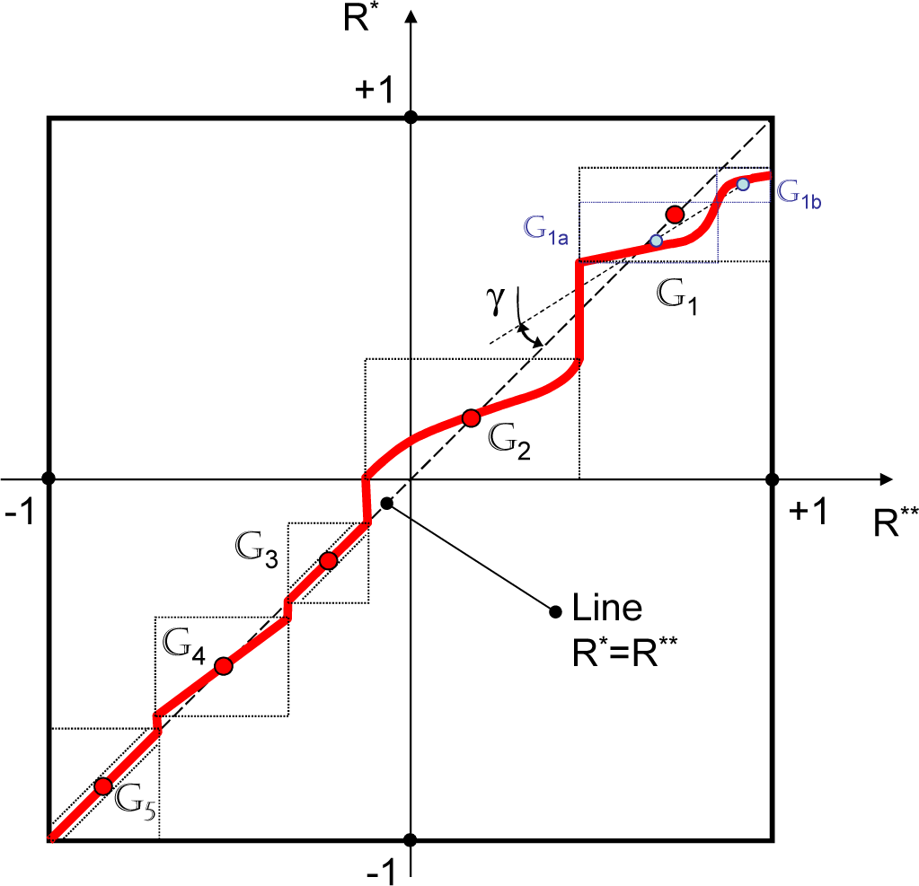
D. Evolutionary Intransitivity
This section considers characterisation of intransitivity in competitive evolving systems (i.e., systems developing in time due to competition between the elements [5–7]). The weight g(Ci) > 0 is proportional to the probability of selecting element Ci for competition.
D.1. Competitive Evolution
The use of current rankings can be illustrated by evolution of competitive systems, which is considered in this subsection. Consider a system of n elements (particles) that evolve in time due to competition between these elements and, consequently, have a preference defined for these elements (which is referred to as the primary preference). The focus of the present consideration is competition steps (not involving mutations). In this case evolution of the system due to competition is determined by the current ranking according to the equation [5]
where f(A) is probability of having an element at location A, λ is a constant depending on the time step and R∗(A) is the primary current ranking defined with the weight g(B) = f(B)ψ(B), which is proportional to the probability ψ(B) of selecting element B for competitive mixing. (Generally, this selection weight can depend on both A and B, that is ψ = ψ(A,B) as considered in [5] but this is not needed in the present work). Since selection of elements for mixing is stochastic, the process of competition requires a probabilistic description (the fluctuations with respect to the averages are not considered). This is achieved with the use of probability f, which can be initially set according to the location of n stochastic particles, which numerically represent f by a large set of delta-functions, before the competition steps. Mutation step, which is not considered here, would make this distribution continuous. As noted above, isolated elements g(…) = 0 are not of interest and all elements are presumed to be connected by competition.
Let
denote the state of the system at time t so that the subscript “t” relates quantities to this state. The following proposition indicates the direction of the competition steps:
Proposition D1 Competition (transitive or intransitive) results in improved competitiveness with respect to the current distribution f, that is for t2 = t1 + dt
First, we note that
due to the antisymmetric properties of co-ranking R(A,C). The substitution of
, where df is determined from Equation (D1), into Equation (D2) results in
since f, ψ2 and (R∗)2 are non-negative. Fluctuations that can be present in the system due to random particle selection are not considered here. Note that, in intransitive systems, competitiveness increases only with respect to the current distribution and improvement is not necessarily achieved when viewed from a different perspective, that is
may decrease in time for some reference groups
. It is common to have a view attached to current distribution—this, according to Proposition D1, produces the impression that competitiveness is improved by the competition but, in intransitive systems, the actual result might be different if viewed from a different perspective (i.e., using a different reference set). The effect of mutation steps (which is not considered here) on competitiveness is typically negative.
D.2. Evolutionary Intransitivity in Simulations of the Risk/benefit Dilemma
The standard deviation of the primary and secondary rankings
is a measure of deviation from transitivity in evolution of competitive systems specified by Equation (D2). Parameter Ω is thus referred to as evolutionary intransitivity parameter; Ω is plotted in Figure 9 by dashed lines. In intransitive simulations, Ω is small for most of the time and the evolution is quite close to being transitive (see Figure 10a–c). If Ω is close to zero, the underlying preference is, effectively, currently transitive. These rules Equation (68), however, are very different from the transitive rules given by Equation (68) as shown in Figure 10d–f. When the system approaches a point of maximal benefit, the evolutionary intransitivity parameter increases, indicating the approaching collapse of the high-benefit/high risk state. Thus evolution of the system may seem transitive most of the time but detection of increasing intransitivity warns of imminent catastrophe resulting in collapse of the benefit.
E. Summary of the Terms Characterising Intransitivity
We distinguish the following types of intransitivity:
- By strictness of the preference:
- – strict intransitivity: there exists A≻B≻C≻A
- – semi-strict intransitivity: there exists A≻C1≻…≻Ck≻A but intransitivity is not strict
- – semi-weak intransitivity: there exists A≻B~C≻A but intransitivity is not semi-strict
- – weak intransitivity: there exists A∼B∼C≻A but intransitivity is not semi-weak
- By localisation:
- – local intransitivity (combined with global transitivity)
- – global intransitivity (combined with local transitivity)
- – strong intransitivity (strict and both local and global)
- By explicit presence:
- – absolute transitivity: any kind of intransitivity is impossible under the given preference rules, implying existence of absolute utility or ranking
- – potential intransitivity: intransitivity does not necessarily show on the current set of elements but may appear when conditions are changed
- – current intransitivity or current transitivity: indicate the properties of preferences on the current set of elements
- – near-transitive evolution: evolution of an intransitive system that, within a fixed time interval, can be reasonably approximated by evolution of a transitive system
Weak and semi-weak intransitivity is not a prominent type of intransitivity since the preference in this case can be represented as a coarsening of a transitive preference (this representation can be achieved by transitively extending preference “≻” to some of pairs that are originally specified as equivalent). A preference with strict or semi-strict intransitivity can not be represented as a coarsening of any transitive preference.
F. Note on Quantum Preferences
Quantum games and quantum mechanisms of preferences and decision-making are notable extensions of the respective classical approaches that have been repeatedly researched in the recent years [25,27,46].
F.1. Quantum Preferences and Co-Rankings
While conventional strict preference implies that either A preferred over B or vice versa, quantum preferences allow for A≻B and A≺B to be valid at the same time. Here we refer to the superposition states which have the quantum wave function Ψ and the quantum density matrix
specified by
or to the mixed states with the wave function Ψ and the quantum density matrix
are taking the forms
Here, we use the conventional quantum ket notations |…〉 and imply normalisation condition
. The symbol
used here is not related to co-ranking ρ. In this section, the overbar denotes the complex conjugates. The strict quantum preferences can be treated as qubits.
In order to distinguish superposition and mixed states in terms of wave functions, we deploy random phases θj = e−iωj where ωj (j = 1, …) are random angles, which are uniformly and independently distributed between −π and π. A mixture of quantum states is interpreted here as an entanglement with special quantum states |θj] representing the random phases. These states have only one operation applicable to these states and resulting in a physically measurable quantities—the scalar product:
The random phase notations are generally equivalent to the corresponding notations using density matrices but random phases can be convenient for specification of mixed states when using wave functions is preferred over deploying density matrices. The random phases is only a convenient notation but not a physical theory that answers the question whether a larger system (or the whole Universe) is physically in a superposition state or a mixed state. The random phases do not have energy and do not evolve in time (in unitary quantum mechanics). The notations based on wave functions are often more explicit and transparent than the equivalent notations based on density matrices (see Appendix of [47] for details and discussion).
In the case of superposition state, both the relative magnitudes
and phases arg(c2) − arg(c1) of complex amplitudes c1 and c2 affect the quantum state. In the case of a mixed state, the phases are not important as they are randomised by θ1 and θ2 but the relative magnitudes
determine the state: the effect of a mixed state is similar to classical probabilities P2 = |c2|2 and P1 = |c1|2, P1 + P2 = 1.
The physical magnitude of the preference is determined by the Hermitian preference operator ℝ, which is specified by the matrix
taking the form
This operator corresponds to the indicator co-ranking R in conventional preferences. For both superposition state Equation (F1) and mixed state Equation (F2), the magnitude of the preference is given by
The quantum preference models the state of mind before a decision of selecting A or B from the set of {A,B} takes place. The instance of decision is marked by the collapse of the wave function converting the system in one of the states, |A ≻ B〉 or |B ≻ A〉 with respective probabilities P1 = |c1|2 and P2 = |c2|2. These probabilities are the same for superposition states Equation (F1) and mixed states Equation (F2).
Demonstrating existence of quantum mechanisms in cognitive decision making is closely linked to the fundamental possibility of distinguishing superposition states and mixed states as various features of mixed states can be interpreted in terms of classical probabilities and, generally, point to probabilistic but not necessarily quantum effects in evaluation of preferences by the human brain. Only quantum superpositions possess all unique flavours of quantum mechanics. Distinguishing quantum superpositions and quantum mixtures generally requires a measurable value H that corresponds to a Hermitian operator
with non-zero off-diagonal elements. The same effect can be achieved by evolving the preference state with a unitary operator U provided this operator is not trivial and corresponds to a physically observable process. The evolved state
of the measurable preference operator R would generally acquire off-diagonal components. For mixed state Equation (F2), the value of H is, as in the case of classical probabilities, the sum of conditional values
and
multiplied by the respective probabilities P1 and P2. The bra/ket notations are abbreviated here to |A〉 = |A ≻ B〉 and |B〉 = |B≻A〉. In the superposition state Equation (F1), the additional terms with interferences
and
appear in the sum: conditional alternatives do interfere in quantum mechanics. However, it is not completely clear what measurable physical quantities operator
might represent, when the two basic states |A〉 and |B〉 represent alternative preferences, and how experiments distinguishing mixed cognitive states from superimposed cognitive states in decision-making can be carried out.
In the case of weak preferences, which have three possible outcomes, the superposition and mixed wave functions become
while the preference operator
is given by the matrix
F.2. Absolute Ranking in Quantum Case
Consider a set of absolute ranks r1, …, rk. If these ranks are sharp, we can assume that ri = i without loss of generality. The state of a single quantum element is specified by the wave function
where the absolute rank of state |i〉 is r(|i〉) = i, i.e., each element is generally a superposition of different states with different absolute ranks.
If we consider two elements, A and B, the state of the system is a superposition of states
where |i, j〉 denotes |ri(A)〉 |rj(B)〉.
If the states |i, j〉 are ordered so that k1 = (k2 − k)/2 states i > j are followed by k states i = j and then by k1 states states i < j, then the matrix
of the preference co-ranking operator
takes the following form
![Entropy 17 04364f14]() where the size of the matrix is k × k and Î is the k1 × k1 unit matrix while the remaining elements are zeros. The preference co-ranking value is given by
where the size of the matrix is k × k and Î is the k1 × k1 unit matrix while the remaining elements are zeros. The preference co-ranking value is given by
(F11).
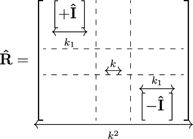
This expression is the same for superimposed and mixed states of the wave function Ψ. We state that A≻B when R(A,B) > 0.
If n quantum elements C1, …,Cn are simultaneously considered, then the wave function takes the form
while the co-ranking of two elements becomes
where
is the set of indices that includes all indices with exception of the indices iq and ip. The probabilities Pij(Cq,Cp) are joint probability distributions of ranks for two elements Cq and Cp. The case of interest when these distributions are independent (separable in quantum terminology) that is for any two elements A and B
In this case each element in quantum formulations becomes very similar to a group with k classical deterministic elements and weights gi = Pi.
The principal difference between deterministic and quantum formulations is that, in the quantum case, existence of absolute ranking does not guarantee transitivity as stipulated in the following proposition
Proposition F1 A quantum (or probabilistic) preference can be intransitive even if it has an absolute ranking.
Indeed, Figure F1 illustrates the case of three elements A, B and C with independent probability distributions Pi(A), Pi(B) and Pi(C) over k = 9 ranks i = 1, …, 9. This case follows the dice example shown in Figure 1b. It can be seen that
since R(B,A) = R(C,B) = R(A,C) = 1/9.
Figure F1.
Intransitive A ≺ B ≺ C ≺ A preference for quantum/probabilistic elements with absolute ranking ri, where Pi indicates probability of state i.
Figure F1.
Intransitive A ≺ B ≺ C ≺ A preference for quantum/probabilistic elements with absolute ranking ri, where Pi indicates probability of state i.

References
- Von Neumann, J.; Morgenstern, O. Theory of Games and Economic Behavior; Princeton University Press: Princeton, NJ, USA, 1953. [Google Scholar]
- Caratheodory, C. Studies in the foundation of thermodynamics. Math. Ann. 1909, 67, 355–386. [Google Scholar]
- Lieb, E.H.; Yngvason, J. The Entropy of Classical Thermodynamics. In Entropy; Greven, A., Keller, G., Warnecke, G., Eds.; Princeton University Press: Princeton, NY, USA, 2003; Chapter 8; pp. 147–195. [Google Scholar]
- Gyftopoulos, E.; Beretta, G. Thermodynamics. Foundations and Applications; Dover Publications: Mineola, NY, USA, 1991. [Google Scholar]
- Klimenko, A.Y. Mixing, entropy and competition. Phys. Scr. 2012, 85, 068201. [Google Scholar]
- Klimenko, A.Y. Complex competitive systems and competitive thermodynamics. Phil. Trans. R. Soc. A 2013, 371. [Google Scholar] [CrossRef]
- Klimenko, A. Entropy and Equilibria in Competitive Systems. Entropy 2014, 16, 1–22. [Google Scholar]
- Allais, M. Le Comportement de l’Homme Rationnel devant le Risque: Critique des Postulats et Axiomes de l’Ecole Americaine. Econometrica 1953, 21, 503–546. [Google Scholar]
- Edwards, W. The prediction of decisions among bets. J. Exp. Psychol. 1955, 50, 201–214. [Google Scholar]
- Kahneman, D.; Tversky, A. The psychology of preferences. Sci. Am. 1982, 246, 160–173. [Google Scholar]
- Quiggin, J. A theory of anticipated utility. J. Econ. Behav. Organ. 1982, 3, 323–343. [Google Scholar]
- Fishburn, P.C. Transitive measurable utility. J. Econ. Theory 1983, 31, 293–317. [Google Scholar]
- Tversky, A.; Kahneman, D. Advances in prospect theory: Cumulative representation of uncertainty. J. Risk Uncertain. 1992, 5, 297–323. [Google Scholar]
- Abe, S. Heat and generalized Clausius entropy of nonextensive systems 2000. arXiv:cond-mat/0012115.
- Tsallis, C. Nonextensive Statistical Mechanics and Thermodynamics: Historical Background and Present Status. In Nonextensive Statistical Mechanics and Its Applications; Abe, S., Okamoto, Y., Eds.; Springer: New York, NY, USA, 2001; pp. 3–98. [Google Scholar]
- Hanel, R.; Thurner, S. When do generalized entropies apply? How phase space volume determines entropy. Europhys. Lett. 2011, 96, 50003. [Google Scholar]
- de Condorcet, N. Essay on the Application of Analysis to the Probability of Majority Decisions; De L’imprimerie Royale: Paris, France; p. 1785.
- Tversky, A. Intransitivity of preferences. Psychol. Rev. 1969, 76, 31–48. [Google Scholar]
- Rubinstein, A. Similarity and decision-making under risk: Is there a utility theory resolution to the Allais paradox? J. Econ. Theory 1988, 1, 145–153. [Google Scholar]
- Temkin, L.S. A Continuum Argument for Intransitivity. Philos. Public Aff. 1996, 25, 175–210. [Google Scholar]
- Tullock, G. The Irrationality of Intransitivity. Oxf. Econ. Pap. 1964, 16, 401–406. [Google Scholar]
- Anand, P. The philosophy of intransitive preference. Econ. J. 1993, 103, 337–346. [Google Scholar]
- Debreu, G. Continuity properties of Paretian utility. Int. Econ. Rev. 1964, 5, 285–293. [Google Scholar]
- Nash, J.F. Equilibrium Points in n-Person Games. Proc. Natl. Acad. Sci. USA 1950, 36, 48–49. [Google Scholar]
- Makowski, M. Transitivity vs. intransitivity in decision making process—An example in quantum game theory. Phys. Lett. A 2009, 373, 2125–2130. [Google Scholar]
- Piotrowski, E.W.; Makowski, M. Cat’s dilemma transitivity vs. intransitivity. Fluct. Noise Lett. 2005, 5, L85–L95. [Google Scholar]
- Makowski, M.; Piotrowski, E.; Sladkowski, J. Do Transitive Preferences Always Result in Indifferent Divisions? Entropy 2015, 17, 968–983. [Google Scholar]
- Makowski, M.; Piotrowski, E.W. Decisions in elections-transitive or intransitive quantum preferences. J. Phys. A 2011, 44. [Google Scholar] [CrossRef]
- Persad, G.C. Risk, Everyday Intuitions, and the Institutional Value of Tort Law. Stanf. Law Rev. 2010, 62, 1445–1471. [Google Scholar]
- Katz, L. Rational Choice versus Lawful Choice. J. Inst. Theor. Econ. 2014, 170, 105–121. [Google Scholar]
- Feldman, M.W.; Riley, M.A.; Kerr, B.; Bohannan, B.J.M. Local dispersal promotes biodiversity in a real-life game of rock-paper-scissors. Nature 2002, 418, 171–174. [Google Scholar]
- Reichenbach, T.; Mobilia, M.; Frey, E. Mobility promotes and jeopardizes biodiversity in rock-paper-scissors games. Nature 2007, 448, 1046–1049. [Google Scholar]
- Marshall, L.; Webb, S.D.; Sepkoski, J.J., Jr.; Raup, D.M. Mammalian Evolution and the Great American Interchange. Science 1982, 215, 1351–1357. [Google Scholar]
- Avelino, P.P.; Bazeia, D.; Menezes, J.; de Oliveira, B.F. String networks in ZN Lotka-Volterra competition models. Phys. Lett. A 2014, 378, 393–397. [Google Scholar]
- Lotka, A.J. Undamped oscillations derived from the law of mass action. J. Am. Chem. Soc. 1920, 42, 1595–1599. [Google Scholar]
- Volterra, V. The general equations of biological strife in the case of historical actions. Proc. Edinb. Math. Soc. 1939, 6, 4–10. [Google Scholar]
- Arrow, K.J. Social Choice and Individual Values; Yale University Press: New Haven, CT, USA, 1951. [Google Scholar]
- Ariely, D. Predictably Irrational; HarperCollins: New York, NY, USA, 2008. [Google Scholar]
- Ng, Y.K. Sub-semiorder: A model of multidimensional choice with preference intransitivity. J. Math. Psychol. 1977, 16, 51–59. [Google Scholar]
- Scholten, M.; Read, D. Prospect theory and the forgotten fourfold pattern of risk preferences. J. Risk Uncertain. 2013, 48, 67–83. [Google Scholar]
- Leland, J.W. Similarity judgements and anomalies in intertemporal choice. Econ. Inq. 2002, 40, 574–581. [Google Scholar]
- Lorentziadis, P.L. Preference under risk in the presence of indistinguishable probabilities. Oper. Res. 2013, 13, 429–446. [Google Scholar]
- Klimenko, A.Y. Complexity and intransitivity in technological development. J. Syst. Sci. Syst. Eng. 2014, 23, 128–152. [Google Scholar]
- Klimenko, A.Y. Teaching the third law of thermodynamics. Open Thermodyn. J. 2012, 6, 1–14. [Google Scholar]
- Smith, J.D.; Depew, D.J.; Weber, B.H. Entropy, Information, and Evolution: New Perspectives on Physical and Biological Evolution; MIT Press: Cambridge, MA, USA, 1988. [Google Scholar]
- Meyer, D.A. Quantum Strategies. Phys. Rev. Lett. 1999, 82, 1052–1055. [Google Scholar]
- Klimenko, A.Y. A note on invariant properties of a quantum system placed into thermodynamic environment. Physica A 2014, 398, 65–75. [Google Scholar]
Figure 1.
(a) The rock-paper-scissors game is the best-known example of intransitivity in games; (b) Intransitive dice game where the die thrown by a player wins when it has a higher score than the die thrown by the opposition. The opposite sides of the dice have the same numbers. With the probability of 5/9, die B wins over A, C wins over B, and A wins over C. This dice game is a simple version of Efron’s dice (see article “nontransitive dice” in Wikipedia).

Figure 2.
Comparison of choices A, B and C in case of a fire emergency: (a) “can do more but not less” (dashed line—naive perspective; solid arrows—legal perspective) and (b) “manager’s choice” (arrows indicate the regulation requirements).
Figure 2.
Comparison of choices A, B and C in case of a fire emergency: (a) “can do more but not less” (dashed line—naive perspective; solid arrows—legal perspective) and (b) “manager’s choice” (arrows indicate the regulation requirements).
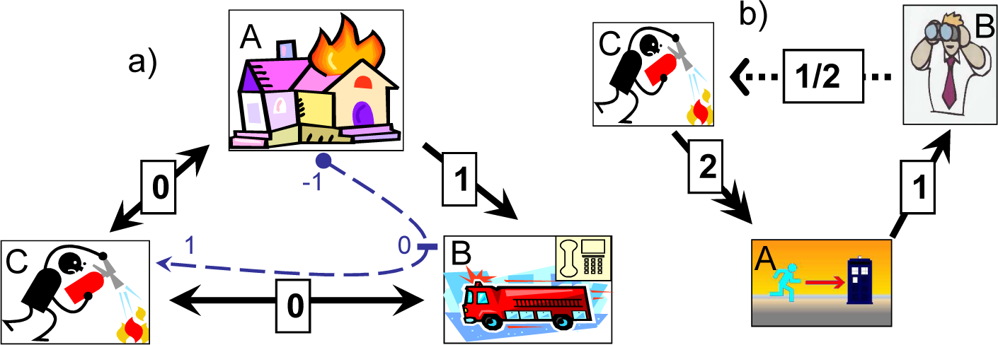
Figure 3.
Presence of intransitivity in the original Lotka–Volterra model.

Figure 4.
Choices A, B and C for The Economist subscription [38]. Dashed blue arrows—value preferences, dotted red arrows—price preference, thick black arrows— overall preferences (shown as the sum of the fractional preferences); the price utility shown in the circles. (a) Original prices; (b) adjusted prices leading to explicit intransitivity

Figure 5.
Intransitivity of fractional (partial) selection criteria when these criteria are known approximately: (a) case of two criteria (b) case of three criteria.
Figure 5.
Intransitivity of fractional (partial) selection criteria when these criteria are known approximately: (a) case of two criteria (b) case of three criteria.

Figure 6.
Estimating the reliable fraction of a utility criterion in presence of Gaussian noise.
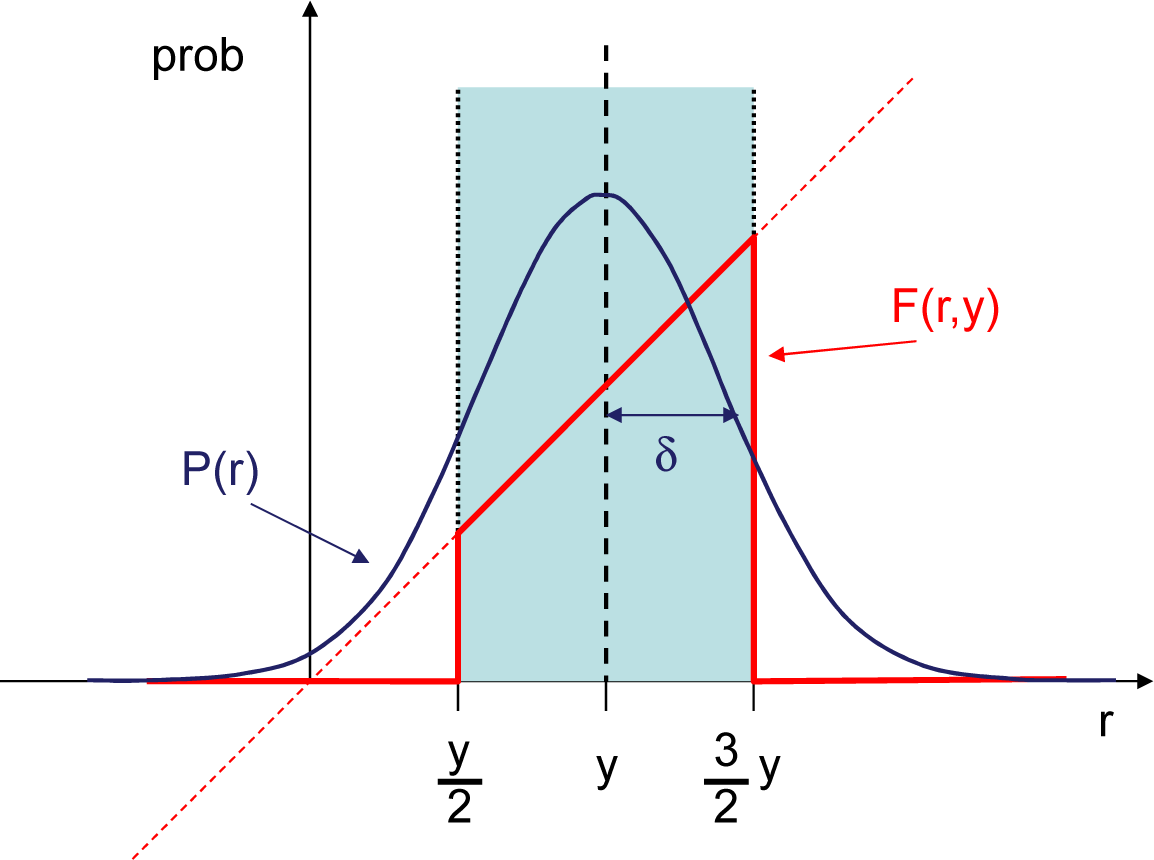
Figure 7.
(a) Co-ranking functions vs. fractional (partial) utility: dotted line—original fine-graded; dashed line—threshold-coarsened; solid line—Gauss-coarsened; (b) Intransitivity due to coarsening in two dimensions: solid line (blue) represents elements X that X∼A and dashed line (red) represents elements X that X∼B for Gauss-coarsened co-rankings with ε(1) = 1 and ε(2) = 1/10. Dotted (blue) line represents elements X that X∼A for fine-graded co-ranking.
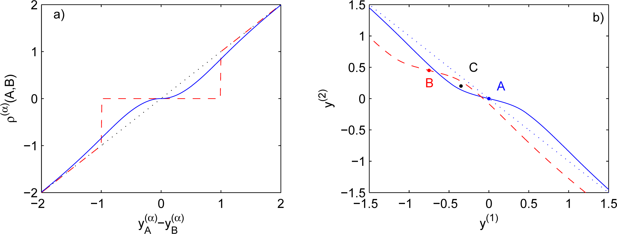
Figure 8.
Schematic of the simulation domain for the risk-benefit dilemma.
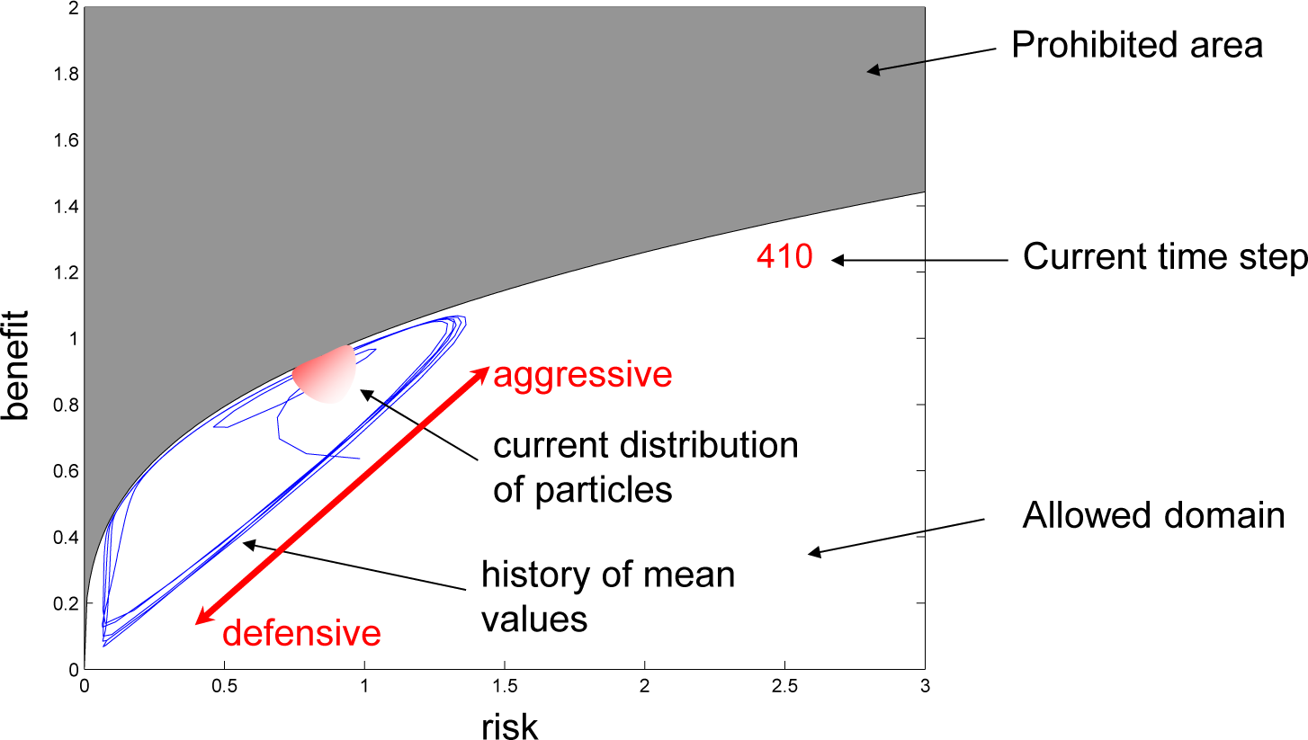
Figure 9.
Simulations of the risk-benefit dilemma. Scale on the left: solid line (blue)—average benefit, dots (black)—equilibrium state in the corresponding transitive competition. Scale on the right: dashed line (red)—evolutionary intrasitivity parameter Ω (see Appendix D). Vertical lines: cases shown in Figure 10.

Figure 10.
The case as in Figure 9: (a,d,g) at 8 time steps; (b,e,h) at 285 time steps; (c,f,i) at 500 time steps. Plots a,b,c: Primary current ranking R* vs. secondary current ranking R** (solid red line). The cases shown are the same as in Figure 10. The solid blue line with dots corresponds to transitive or effectively transitive case where primary and secondary rankings coincide (see Appendix C). Plots d,e,f: Intransitive primary current ranking R* evaluated for co-ranking ρ specified by Equation (70) vs. transitive primary current ranking
evaluated for co-ranking ρ0 specified by Equation (68). Deviations from the solid line with dots indicate differences between current rankings based on ρ and on ρ0. Plots g,h,i: Domain snapshots. Colour shows the primary current ranking R* for each particle according to the colour bar. Plot i: blue line is a 500-step history of mean values; enlarged box is shown as insert.
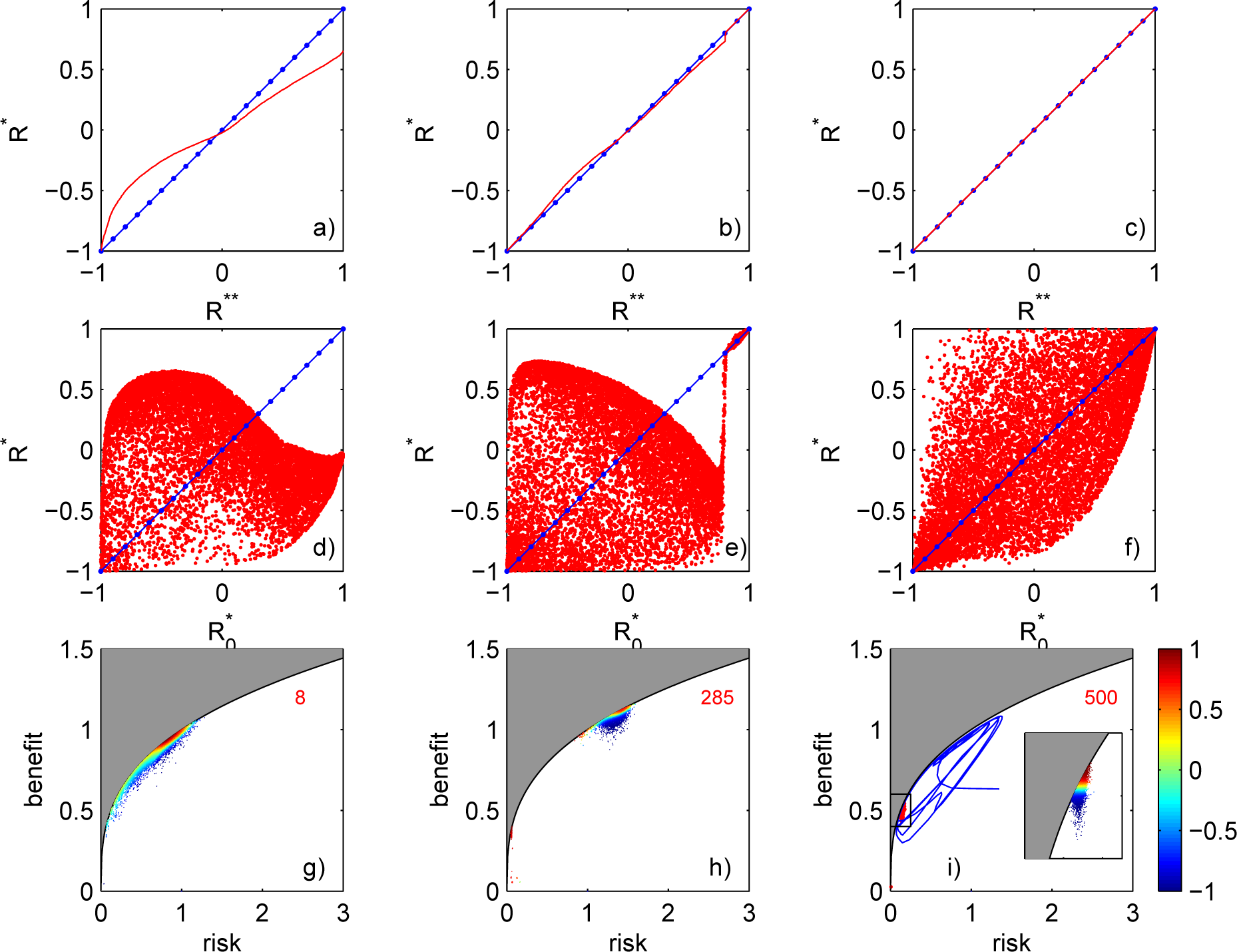
Figure 11.
Intransitive systems that display a degree of similarity with transitive systems: (a) locally intransitive globally transitive system and (b) locally transitive globally intransitive system.
Figure 11.
Intransitive systems that display a degree of similarity with transitive systems: (a) locally intransitive globally transitive system and (b) locally transitive globally intransitive system.
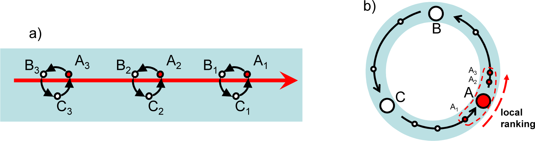
© 2015 by the authors; licensee MDPI, Basel, Switzerland This article is an open access article distributed under the terms and conditions of the Creative Commons Attribution license (http://creativecommons.org/licenses/by/4.0/).
Share and Cite
MDPI and ACS Style
Klimenko, A.Y. Intransitivity in Theory and in the Real World. Entropy 2015, 17, 4364-4412. https://doi.org/10.3390/e17064364
AMA Style
Klimenko AY. Intransitivity in Theory and in the Real World. Entropy. 2015; 17(6):4364-4412. https://doi.org/10.3390/e17064364
Chicago/Turabian StyleKlimenko, Alexander Y. 2015. "Intransitivity in Theory and in the Real World" Entropy 17, no. 6: 4364-4412. https://doi.org/10.3390/e17064364