Detecting Chronotaxic Systems from Single-Variable Time Series with Separable Amplitude and Phase

Abstract

The recent introduction of chronotaxic systems provides the means to describe nonautonomous systems with stable yet time-varying frequencies which are resistant to continuous external perturbations. This approach facilitates realistic characterization of the oscillations observed in living systems, including the observation of transitions in dynamics which were not considered previously. The novelty of this approach necessitated the development of a new set of methods for the inference of the dynamics and interactions present in chronotaxic systems. These methods, based on Bayesian inference and detrended fluctuation analysis, can identify chronotaxicity in phase dynamics extracted from a single time series. Here, they are applied to numerical examples and real experimental electroencephalogram (EEG) data. We also review the current methods, including their assumptions and limitations, elaborate on their implementation, and discuss future perspectives.

1. Introduction

The theory of nonautonomous dynamical systems has increasingly been recognised as a necessity in the treatment of the inherent time-variability of biological systems [1]. Closer inspection of the dynamics observed in nature suggests that previous approaches to the characterization of temporal fluctuations in these observations may be insufficient. At first glance, biological fluctuations may appear random, leading to their description by stochastic models [2]. The complexity observed in biological systems has also led to attempts to treat them with chaos theory [3], however this does not allow for the apparent stability of these systems, irrespective of their initial conditions. Such characteristics of biological oscillators suggests underlying determinism or control of both their amplitudes and frequencies, even with continuous perturbations. This phenomenon of biological systems resisting a natural tendency to disorder was discussed in terms of free energy minimization [4] and separation of internal and external states, but this approach is still based on random dynamics. A closely related, yet more natural, approach is to consider them as nonautonomous systems, which are explicitly time-dependent. Approaches based on reformulation of nonautonomous systems as higher dimensional autonomous systems introduce unnecessary complexity, whilst failing to accurately describe dynamics arising from nature due to the fact that these are open systems, subject to continuous variable external perturbations. Many living systems may be considered as nonautonomous oscillatory systems, with such time-varying dynamics observed in individual mitochondria [5], the cardio-respiratory system [6,7], the brain [8], and blood flow [9].

Although stability of the amplitude dynamics of an oscillator can be achieved with autonomous self-sustained limit cycle oscillators, the frequency of this oscillation could be easily changed by weak external perturbations [10]. To account for a case where this frequency of oscillation is also robust to perturbations, yet time-dependent, a completely new approach is required. Thus, nonautonomous systems with stable, yet time-varying frequencies were recently addressed, and formulated as chronotaxic systems [10–12]. Chronotaxic systems possess a time-dependent point attractor provided by an external drive system. This allows the frequency of oscillations to be prescribed externally through this driver and response system, giving rise to determinism, even when faced with strong perturbations.

Once these properties of the underlying system have been recognised, the next problem is how to infer these dynamics and interactions from direct observations, i.e., via the inverse approach. In a chronotaxic system, particularly one found in nature, whilst the underlying dynamics are defined by the external driver, the system will likely still be affected by other influences and noise. These may mask the chronotaxic dynamics if the correct analytical approach is not applied. For example, the inherent time-variability of the frequency of the dynamics arising from a chronotaxic system means that it cannot be accurately characterized by any method based on averaging. This novel class of systems requires new inverse approach methods, with the focus on the extraction and identification of the dynamics of the drive system, and its influence on the response system. Here, we review the current state of inverse approach methods for the identification of chronotaxicity from a single time series of the response system in which the phase and amplitude dynamics are separable. We then apply these methods to numerically simulated and real experimental data. Section 2 presents the mathematical formulation of chronotaxic systems, Section 3 describes current inverse approach methods and their application to the detection of chronotaxicity. In Section 4, numerical examples are presented to demonstrate the methods, and their assumptions and limitations are discussed. The inverse approach methods are also applied to real experimental data. Finally, Section 5 discusses future directions of the work.

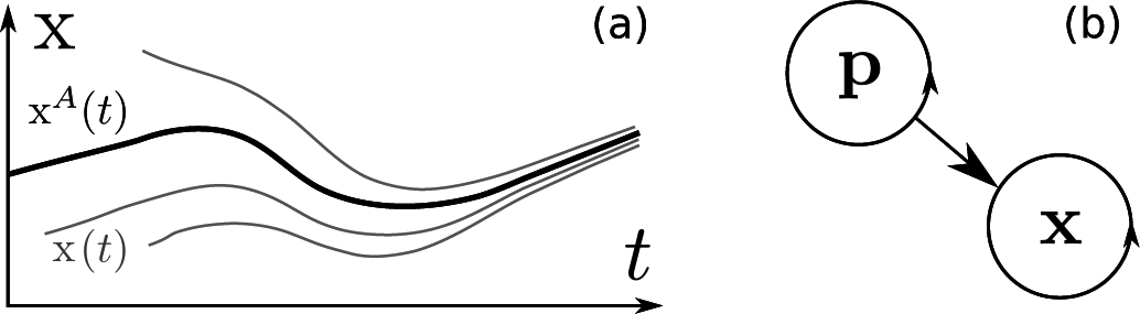
2. Chronotaxic Systems

The crucial concept in the theory of chronotaxic systems is the ability to resist continuous external perturbations. In autonomous systems, such an ability is provided by a stationary steady state, allowing the system to always return to the vicinity of this steady state when continuously externally perturbed. However, only in nonautonomous (thermodynamically open) systems can the position of this steady state change in time, i.e., be outside of equilibrium. In such a case, not only the stationary state of a system, but also its time-dependent dynamics will be able to resist continuous external perturbations. These oscillatory nonautonomous dynamical systems with time-dependent steady states were introduced by Suprunenko et al. [10] and named chronotaxic systems, emphasizing that their dynamics is ordered in time (chronos — time, taxis — order).

Mathematically, nonautonomous dynamical systems and, consequently, chronotaxic systems, are defined by the following system of equations:

$$\dot{\mathrm{p}}=\mathrm{f}\left(\mathrm{p}\right);\dot{\mathrm{p}}=(\mathbf{x},\mathrm{p}),$$

(1)

where p ∈ Rⁿ, x ∈ R^m, f : Rⁿ → Rⁿ, g : R^m × Rⁿ → R^m, in which n and m can be any positive integers. Importantly, the solution x(t, t₀, x₀) of Equation (1) depends on the actual time t as well as on the initial conditions (t₀, x₀), whereas the solution p(t − t₀, p₀) depends only on initial condition p₀ and on the time of evolution t − t₀. The subsystem x is nonautonomous in the sense that it can be described by an equation which depends on time explicitly, e.g., $\dot{\mathbf{x}}=\mathrm{g}\left(\mathbf{x},\mathrm{p}\left(t\right)\right)$. A chronotaxic system is described by x which is assumed to be observable, and p which may be inaccessible for observation, as often occurs when studying real systems. Rather than assuming or approximating the dynamics of p, we focus on the dynamics of x and use only the following simple assumption: system p is assumed to be such that it creates a time-dependent steady state in the dynamics of x, which is schematically shown in Figure 1a.

Therefore, the whole external environment with respect to x is divided into two parts. The first part is given by p which is only that part which makes the system x chronotaxic (defined below), i.e., an unperturbed chronotaxic system. The second part contains the rest of the environment, and is therefore considered as external perturbations.

Firstly, we provide a mathematical formulation of unperturbed chronotaxic systems. The defining component of an unperturbed chronotaxic system is a time-dependent steady state, also called a point attractor, and denoted x^A(t).

Usually, a steady state is defined using a so-called forward limit, when forward time approaches infinity. Assuming that the whole space R^m of x is a basin of attraction, i.e., that for any initial condition x₀ at time t₀ the solution of the system asymptotically approaches the time-dependent steady state x^A, a condition of forward attraction for x^A is the following,

$$\underset{t\to +\infty }{\lim }|\mathbf{x}(t,t_0,{\mathbf{x}}_0)-{\mathbf{x}}^A(t)|=0.$$

(2)

This condition can only be satisfied when the chronotaxic system is not perturbed. However, taking into account the time-dependence of x^A(t), this condition is not satisfactory in terms of defining the time-dependent point attractor. Any solution $\tilde{\mathbf{x}}\left(t,t_0,{\mathbf{x}}_0\right)$ which satisfies Equation (2) with given x^A(t) can also be considered as a time-dependent point attractor. Moreover, when dealing with living systems, it is crucially important to describe stability at the current time t and not in the infinite future. This problem is resolved by employing a condition of pullback attraction, which should also be satisfied by x^A(t) in a chronotaxic system,

$$\underset{t_0\to -\infty }{\lim }|\mathbf{x}(t,t_0,{\mathbf{x}}_0)-{\mathbf{x}}^A(t)|=0.$$

(3)

One can see, that this condition defines a time-dependent point attractor at current time t.

Considering the condition in Equation (3) at all times t > −∞, it follows that the time-dependent point attractor should also satisfy the invariance condition, i.e., the condition that x^A is a solution of the system Equation (1),

$$\mathbf{x}(t,t_0,{\mathbf{x}}^A(t_0))-{\mathbf{x}}^A(t).$$

(4)

Equations (2) and (3) determine asymptotic convergence in the infinite future or starting from the infinite past. Asymptotic convergence allows the dynamics of x(t, t₀, x₀) to deviate from x^A during a certain finite time interval. Thus, during this time-interval the ability to resist continuous external perturbations will be absent. Therefore, in order to characterize the ability of living systems to sustain their time-dependent dynamics at finite time intervals, a chronotaxic system should satisfy the condition of contraction, or equivalently the attraction at all times. This means that in the phase space R^m, x ∈ R^m, there should be a contraction region C(t) such that for any two trajectories x₁, x₂ of a system inside the contraction region x_i(t, t₀, x_0i) ∈ C(t), i = 1, 2, the distance between them can only decrease,

$$\frac{d}{dt}|{\mathbf{x}}_1(t,t_0,{\mathbf{x}}_{1,0})-{\mathbf{x}}_2(t,t_0,{\mathbf{x}}_{2,0})|<0.$$

(5)

However, in general the contraction region C(t) can be finite, and different trajectories can eventually leave this region. Therefore, in a chronotaxic system the contraction region should contain a finite area A^′, A^′ ⊂ C, such that solutions of the system starting in A^′ never leave it, ∀t₀ < t, ∀x₀ ∈ A^′(t₀), x(t, t₀, x₀) ∈ A^′ (t).

In such a case, fulfillment of these conditions guarantees that the time-dependent point attractor x^A is located inside the area A^′ inside the contraction region C.

Alternatively, the trajectory x^A(t) can be viewed as a linearly attracting uniformly hyperbolic trajectory [13], so that the distance between a neighboring trajectory and x^A(t) can only decrease in an unperturbed chronotaxic system. For more details and for relations between chronotaxic and other dynamical systems see Reference [12]. A simple example of an unperturbed chronotaxic system is given by unidirectionally coupled phase oscillators with unwrapped phase φ_x ∈ (−∞, ∞) driven by a phase φ_p ∈ (−∞, ∞):

$${\dot{\phi }}_{\mathbf{x}}={\omega }_0(t)-\epsilon (t)\sin ({\phi }_{\mathbf{x}}-{\phi }_{\mathrm{p}}(t)),$$

(6)

where ${\dot{\phi }}_{\mathrm{p}}\left(t\right)=\omega \left(t\right)$.

The point attractor will exist if the condition of chronotaxicity [11] is fulfilled, |ε(t)| > |ω₀(t)−ω(t)|.

As an example, for a particular choice ε(t) = ω(t) > 0 and ω₀(t) = 0, the equation can be integrated, and the limit t₀ → −∞ can be calculated, leading to the explicit expression for a time-dependent point attractor of an unperturbed chronotaxic system, ${\phi }_{\mathbf{x}}^A\left(t\right)={\phi }_{\mathrm{p}}\left(t\right)-\pi /2+2\pi k$, and k is any integer.

It should be noted that the dynamics of p can be complex, stochastic, or chaotic, provided that the above conditions are met. Nevertheless, the dynamics of x will be determined by the dynamics of p, and therefore it will be deterministic, at least in unperturbed chronotaxic systems. When considering perturbed chronotaxic systems, for simplicity it is sufficient to consider perturbations only to the x component, as any perturbations to p can be included in its dynamics assuming that x does not influence p. In perturbed chronotaxic systems, which model real life systems, the general external perturbations will create complex dynamics of x with a stochastic component. Such dynamics may look very complex: perturbations can push trajectories away from the contraction region, therefore they can temporarily deviate before they converge. Despite this, due to the existence of the contraction region, the system will resist continuous external perturbations. The time-dependent dynamics of a perturbed chronotaxic system will be very close to the dynamics of the unperturbed chronotaxic system provided the perturbations are weak enough. In the case of very strong continuous perturbations, such perturbations may override the driving system p, and become effectively a new driver, causing the initial point attractor of the chronotaxic system to disappear. However, it may be restored once the perturbations again become sufficiently weak.

Thus, when perturbations do not destroy the chronotaxic properties of a system, the stable deterministic component of its dynamics can be identified, as will be shown below. This reduces the complexity of the system, allowing us to filter out the stochastic component and focus on deterministic dynamics and interactions between system x and its driver p, [10,14]. For such complex systems as living systems, it has the potential to extract properties of the system which were previously neglected.

3. Inverse Approach for Chronotaxic Systems

3.1. Inverse Approaches to Nonautonomous Dynamical Systems

A wide range of observed properties in living systems can be explained by considering them as nonautonomous. Despite this, difficulties in their analysis as such have led to many unsuccessful attempts to apply methods more suited to autonomous systems. From a single time series arising from a dynamical system, inverse approach methods can be used to infer the underlying dynamics of this system, in terms of phase or amplitude. In deterministic systems, phase space analysis is usually the first point of call, i.e., reconstruction of the attractor in phase space. This can be achieved with only a single time series using embedding, in which the dimensions of the reconstructed attractor are composed of time-delayed versions of the data in the time series [15]. This approach works well for autonomous systems, but does not consider the possibility of time-dependent attractors [1]. Phase space methods are particularly suited to the treatment of the dynamics observed in chaotic systems. In contrast, nonautonomous systems appear very complex in phase space. To incorporate time-dependence into these systems, extra dimensions in phase space are required, introducing unnecessary complexity to the problem.

In the case that there is only one oscillation in the time series, the Hilbert transform can be applied to obtain the complex analytic signal, from which the instantaneous phase can be determined directly. If the time series contains more than one component of interest, for example different oscillatory modes, it can be decomposed into its constituent parts using a method such as empirical mode decomposition (EMD), in which peak/trough detection is used to create upper and lower envelopes. From these, a trend is defined and subtracted from the signal to produce a series of intrinsic mode functions, each one representing an oscillatory component of the time series [15]. However, there are some limitations when applying EMD to nonstationary data.

Many signal analysis methods assume stationarity of the frequency distribution of the data, but in nonautonomous systems this assumption is not valid. Single variable time series, particularly those from living systems, must be treated as arising from nonautonomous dynamical systems, due to time-dependent influences of variables other than the one under study. Approaches based on windowing have been applied in order to attempt to treat time variability in data, but these potentially lose crucial information. For example, in phase space reconstruction the window may not be of a sufficient size to capture the whole of the attractor, or its variations in time. Application of the Fourier transform to nonstationary data will result in a blurred or misleading power spectra, severely limiting its usefulness. The windowing approach has been applied here with some success, in the form of the Short Time Fourier transform (STFT), but the use of windowing leads to limitations; the better the time resolution, the worse the frequency resolution (known as the Gabor limit [16]). In addition, the fixed time–frequency relationship at all scales in a windowed Fourier transform severely limits its usefulness for the analysis of low frequency oscillations. This problem can be addressed by using the continuous wavelet transform (CWT), which provides a logarithmic frequency scale (see Section 3.3). The CWT is based on wavelets rather than the sines and cosines used in Fourier based methods. The simultaneous observation of the time and frequency domains is extremely useful in the visualization of dynamical systems and their time evolution. As a result, development of wavelet-based methods specifically for the treatment of time-dependent dynamics is now a very active field of research [15], including wavelet phase coherence [17], the synchrosqueezed transform [18,19] and wavelet bispectrum.

In addition to determining the characteristics of the underlying dynamics of single nonautonomous oscillatory modes, inverse approach methods are also used to decompose their interactions. One of the most well known characteristics of interacting systems is synchronization between oscillatory components, i.e., a fixed relationship between their phases or amplitudes. Once the phases of oscillations have been extracted from a time series, a measure of phase synchronization can be calculated using synchronization indices or phase coherence [15]. However, these methods do not account for time-varying synchronization. Dynamical Bayesian inference is able to detect time-varying synchronization in a system, whilst simultaneously inferring the direction of coupling and time-evolving coupling functions [20,21]. In the time–frequency domain, wavelet phase coherence can be used to monitor phase relationships over time and frequency by utilising the phase information obtained from the continuous wavelet transform [15,17]. In a similar way, couplings between oscillators can be detected and quantified using wavelet bispectrum [22]. The ability of these methods to directly take into account the time-varying characteristics of data makes them ideal for application to nonautonomous systems.

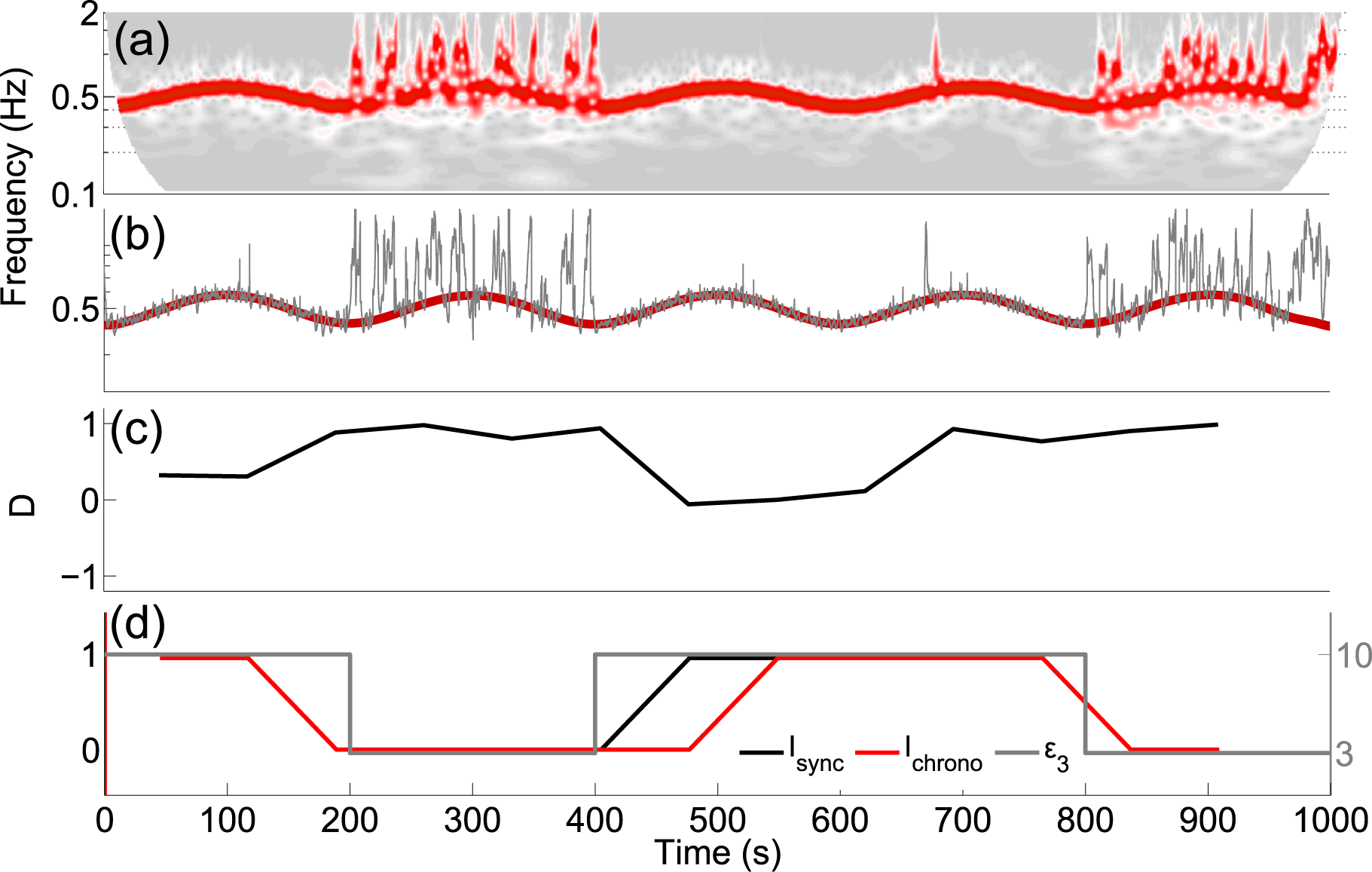
3.2. Detecting Chronotaxicity

Here we present two distinct inverse approach methods which may be utilised in the detection of chronotaxicity: phase fluctuation analysis (PFA) and dynamical Bayesian inference. It should be noted that the current methods are only applicable to phase dynamics in the context of the detection of chronotaxicity, i.e., we focus on the ability of the time-varying frequency to resist continuous external perturbations. The two methods rely on a different inferring basis. Phase fluctuation analysis provides a measure of statistical effects observed in a signal, whilst the dynamical Bayesian inference method infers a model of differential equations and gives a measure of dynamical mechanisms, i.e., the evaluation of chronotaxicity relies on the inferred parameters of the model. PFA is said to infer a functional connectivity, while the dynamical Bayesian inference method infers effective connectivity [23]. The optimal method to use depends on the characteristics of the data, as detailed below.

It is possible to detect whether a system is chronotaxic or not by observing the distribution of the fluctuations in the system relative to its unperturbed trajectory. This comes from the fact that if the original distribution of the perturbations is known, then the stability of the system relative to the unperturbed trajectory (which by definition follows the time-dependent point attractor in a chronotaxic system) can be determined from how these perturbations grow or decay over time. For example, take the non-chronotaxic phase oscillator [24]

$${\dot{\phi }}_{\mathbf{x}}={\omega }_0(t)+\eta (t),$$

(7)

where ω₀(t) is the time-dependent natural frequency and the observed phase ϕ_x is perturbed by noise fluctuations η(t). Integrating we find,

$${\phi }_{\mathbf{x}}={\displaystyle \int {\omega }_0(t)dt}+{\displaystyle \int \eta (t)dt}.$$

(8)

Assuming that ω₀(t) > 0 and η(t) is an uncorrelated Gaussian process, this means that the dynamics of φ_x will consist of a monotonically increasing phase perturbed by a random walk noise (Brownian motion). However, the situation is different for a chronotaxic phase oscillator, e.g.,

$$\begin{array}{l}{\dot{\phi }}_{\mathrm{p}}={\omega }_0(t),\\ {\dot{\phi }}_{\mathbf{x}}=\epsilon {\omega }_0(t)\sin ({\phi }_{\mathrm{p}}-{\phi }_{\mathbf{x}})+\eta (t),\end{array}$$

(9)

where φ_p is an external phase and |ε| > 1. In this case the stability provided by the point attractor causes each noise perturbation to decay over time, preventing η(t) from being integrated over to the same extent. The perturbations still do not decay instantly, as the system takes time to return to the point attractor, meaning that some integration of the noise still takes place. However, the size of the observed perturbations over longer time scales is greatly reduced, causing a change in the overall distribution from that expected for Brownian motion.

3.3. Extracting the Perturbed and Unperturbed Phases

The first problem of generating a method based on the above principle is how to extract both the perturbed and unperturbed phases of the system from an observed time series. This usually requires the separation of the amplitude and phase for an oscillation in the time series, which is possible using time–frequency domain analysis [15]. The analytic signal generated by the Hilbert transform can also be used, but this requires corrections for nonlinear oscillations and cannot be used when more than one oscillation is present in the time series [14,25,26]. Additionally, the use of the Hilbert transform requires the use of protophase-to-phase conversion [26].

A time–frequency representation with an optimal frequency resolution of the time series f(t) of length L is provided by the continuous wavelet transform [27],

$$W_T(s,t)={\displaystyle {\int }_0^L\mathrm{\Psi }(s,u-t)f(u)du,}$$

(10)

where Ψ(s, t) is the mother wavelet, which is scaled according to the parameter s to change its frequency distribution and time-shifted according to t. The Morlet wavelet is a commonly used mother wavelet and is defined as [28],

$$\mathrm{\Psi }(s,t)=\frac{1}{\sqrt[4]{\pi }}\left(e^{\frac{2\pi i{f}_{0}t}{s}}-e^{-\frac{2\pi f_0^2}{2}}\right)e^{-\frac{t^2}{2s^2}},$$

(11)

where the corresponding frequency is given by 1/s and f₀ is a parameter known as central frequency which defines the time/frequency resolution [27].

Oscillations can be traced in W_T (s, t) using either a ridge-extraction method [29,30] or the synchrosqueezed wavelet transform (SWT) [18]. These extraction methods can be used to estimate the instantaneous frequencies of the oscillatory components in a time series, allowing identification of harmonics, which can be used to determine the intra-cycle dynamics. The phase φ_x of the observed system is then arg(W_T (s, t)), where s and t denote the positions of the oscillation in the s − t plane.

With the estimated perturbed phase ${\phi }_{\mathbf{x}}^{\ast }$ extracted, further work is needed to obtain the unperturbed phase ${\phi }_{\mathbf{x}}^{A\ast }$. In particular, it is difficult to separate the dynamics corresponding to ${\phi }_{\mathbf{x}}^A$ from the effect of the noise perturbations η(t). This task is simplified by assuming that the dynamics of ${\phi }_{\mathbf{x}}^A$ are confined to time scales larger than a single cycle and that the noise is either weak or comparable in magnitude to these dynamics.

With these assumptions, an estimate of ${\phi }_{\mathbf{x}}^A$ can be found by filtering out high frequency components of ${\phi }_{\mathbf{x}}^{\ast }$. However, such a filter should not smooth over the dynamics of ${\phi }_{\mathbf{x}}^A$. An optimal way of removing these high frequency noise fluctuations without affecting the unperturbed dynamics is to instead smooth over the frequency extracted from the wavelet transform [15]. This provides the estimated angular velocity ${\phi }_{\mathbf{x}}^A$, which can in turn be integrated over time to give the estimated phase of the driver ${\phi }_{\mathbf{x}}^{A\ast }$. For further methodological details on phase extraction see Section 4.2.

3.4. Dynamical Bayesian Inference

One approach to the detection of chronotaxicity is the application of dynamical Bayesian inference to the extracted perturbed $({\phi }_{\mathbf{x}}^{\ast })$ and unperturbed $({\phi }_{\mathbf{x}}^{A\ast })$ phase estimates in order to model their interactions. In dynamical systems Bayesian inference can simultaneously detect time-varying synchronization, directionality of coupling and time-evolving coupling functions [20,21]. The characteristics of these coupling functions between ${\phi }_{\mathbf{x}}^{\ast }$ and ${\phi }_{\mathbf{x}}^{A\ast }$ may reveal the dynamic mechanisms of the system in terms of chronotaxicity. Bayesian inference is able to track time-dependent system parameters, meaning that it is particularly useful for the detection of chronotaxicity in systems which move in and out of a chronotaxic state.

Following extraction of phases from the continuous wavelet transform, as described in Section 3.3, we assume their dynamics is described by [14,20,21]

$${\dot{\phi }}_i={\omega }_i+f_i({\phi }_i)+g_j({\phi }_i,{\phi }_j)+\xi (t),$$

(12)

where ω_i is the natural frequency of the oscillation, f_i(φ_i) are the self-dynamics of the phase, g_i(φ_i, φ_j) are the cross couplings, and ξ(t) is a two-dimensional white Gaussian noise 〈ξ_i(t)ξ_j(τ)〉 = δ(t − τ)E_ij. Based on the periodic nature of the system, the basis functions are modeled using the Fourier bases

$$f_i({\phi }_i)={\displaystyle \sum _{k=-\infty }^{\infty }{\tilde{a}}_{i,2k}\sin (k{\phi }_i)+{\tilde{a}}_{i,2k+1}\cos (k{\phi }_i),}$$

(13)

and

$$g_i({\phi }_i,{\phi }_j)={\displaystyle \sum _{s=-\infty }^{\infty }{\displaystyle \sum _{r=-\infty }^{\infty }{\tilde{b}}_{i,r,s}{e}^{2\pi ir{\phi }_i}{e}^{2\pi is{\phi }_j},}}$$

(14)

where k, r, s ≠ 0. In practice, it is reasonable to assume that the dynamics will be well described by a finite number of Fourier terms, denoted A_i,k(φ_i, φ_j). The corresponding parameters from ${\tilde{a}}_i$ and ${\tilde{b}}_i$ then form the parameter vector $c_k^{(i)}$. The inference of these parameters utilises Bayes’ theorem,

$$px(\mathcal{M}|\chi )=\frac{\ell (\chi |\mathcal{M})p_{prior}(\mathcal{M})}{\int \ell (\chi |\mathcal{M})p_{prior}(\mathcal{M})d\mathcal{M}},$$

(15)

where $p_{\chi }\left(\mathcal{M}|\chi \right)$ is the posterior probability distribution and $\ell \left(\chi |\mathcal{M}\right)$ is the likelihood function for the values of the model parameters $\mathcal{M}$ given the data $\chi$, and $p_{prior}\left(\mathcal{M}\right)$ is a prior distribution. The negative log-likelihood function is

$$S=\frac{N}{2}\ln |E|+\frac{h}{2}{\displaystyle \sum _{n=0}^{N-1}\left(c_k^{(l)}\frac{\partial A_{l,k}(\phi {\cdot }_{,n})}{\partial {\phi }_l}+[{\dot{\phi }}_{i,n}-c_k^{(i)}{A}_{i,k}(\phi {\cdot }_{,n}^{\ast })]{(E^{-1})}_{i,j}[{\dot{\phi }}_{j,n}-c_k^{(j)}{A}_{j,k}(\phi {\cdot }_{,n}^{\ast })]\right)},$$

(16)

with implicit summation over repeated indices k, l, i, j. The log-likelihood is a function of the Fourier coefficients of the phases [20].

Assuming a multivariate normal distribution as the prior for parameters $c_k^{(i)}$ with means $\overline{c}$ and covariances Σ = Ξ⁻¹, the stationary point of S can be calculated recursively from

$$\begin{array}{l}{E}_{i,j}=\frac{h}{N}[{\dot{\phi }}_{i,n}-c_k^{(i)}{A}_{i,k}(\phi {\cdot }_{,n}^{\ast })][{\dot{\phi }}_{j,n}-c_k^{(j)}{A}_{j,k}(\phi {\cdot }_{,n}^{\ast })],\\ c_k^{(i)}={({\mathrm{\Xi }}^{-1})}_{kw}^{i,l}{r}_w^{(l)},\\ r_w^{(l)}={({\mathrm{\Xi }}_{prior})}_{kw}^{(i,l)}{c}_w^{(l)}+h{A}_{i,k}(\phi {\cdot }_{,n}^{\ast }){(E^{-1})}_{ij}{\dot{\phi }}_{j,n}-\frac{h}{2}\frac{\partial A_{l,k}(\phi {\cdot }_{,n})}{\partial \phi l},\\ {\mathrm{\Xi }}_{kw}^{i,j}={\mathrm{\Xi }}_{priorkw}^{i,j}+h{A}_{i,k}(\phi {\cdot }_{,n}^{\ast }){(E^{-1})}_{ij}{A}_{j,w}(\phi {\cdot }_{,n}^{\ast }).\end{array}$$

(17)

These are calculated within a moving time window, with the current prior depending on information from the posterior of the previous window. The inferred parameters of the basis functions can be used to determine whether synchronization results. The presence of synchronization provides evidence that the system is chronotaxic, however it remains unclear from which coupling function the stability arises without calculating the direction of coupling [31],

$$D=\frac{{ϵ}_{12}-{ϵ}_{21}}{{ϵ}_{12}+{ϵ}_{21}},$$

(18)

where

$$\begin{array}{l}{ϵ}_{12}=\sqrt{c_2^2+c_4^2+\dots ,}\\ {ϵ}_{21}=\sqrt{c_1^2+c_3^2+\dots ,}\end{array}$$

(19)

are the Euclidean norms of the parameters. The odd parameters correspond to the coupling terms inferred for φ₁ in the direction 2 → 1, and the even parameters correspond to the coupling terms inferred for φ₂ in the direction 1 → 2. See [32] for further details and an in depth tutorial on dynamical Bayesian inference and its implementation.

In summary, Bayesian inference is applied to ${\phi }_{\mathbf{x}}^{\ast }$ and ${\phi }_{\mathbf{x}}^{A\ast }$, following their extraction from the time series (see Section 3.3). The time evolution of the coupling parameters for each phase is inferred and these are used to determine the synchronization state of the system, and the direction of coupling between the phases. In a chronotaxic system we require the driver and response systems to be almost or fully synchronized, and also that the direction of coupling is only from the driver ${\phi }_{\mathbf{x}}^A$ to φ_x.

The basis of this method is the calculation of the synchronization and direction of coupling of the system in order to determine chronotaxicity. However, the more synchronized the driver is with the response system, the less information flow between the two. With less information from which to infer parameters, most directionality methods, including Bayesian inference, become less reliable, and whilst synchronization may still be accurately detected, the direction of coupling will become less accurate the closer the system gets to synchronization. With frequent external perturbations, intermittent transitions, and moderate dynamical noise, there is greater information flow, and thus the inference is more precise, but this cannot be assumed in chronotaxic systems. In real systems, the synchronization state is not known beforehand, thus a more robust method is required, which can identify chronotaxicity even in systems close to synchronization.

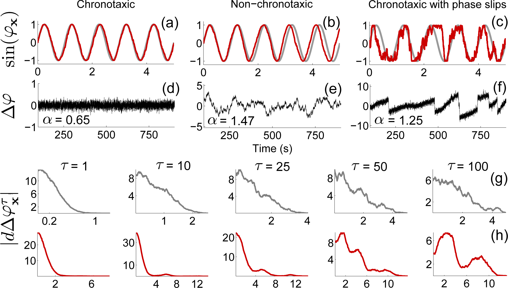
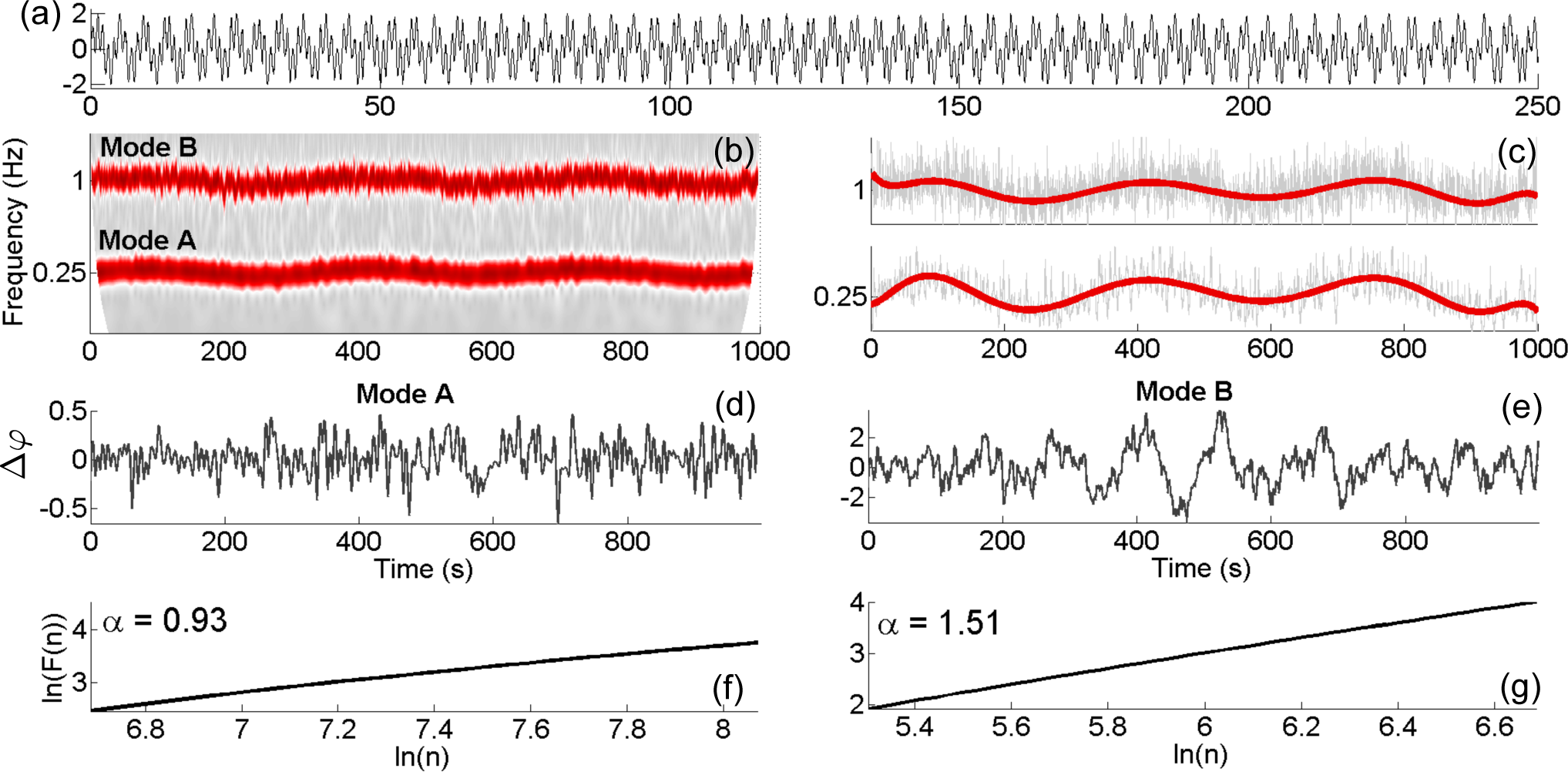
3.5. Phase Fluctuation Analysis

Phase fluctuation analysis is effective even when φ_x and φ_p are almost synchronized. Given the estimates of φ_x and ${\phi }_{\mathbf{x}}^A$, the next step is to analyse $\mathrm{\Delta }{\phi }_{\mathbf{x}}={\phi }_{\mathbf{x}}^{\ast }-{\phi }_{\mathbf{x}}^{A\ast }$ to find the distribution of fluctuations in the system relative to the unperturbed trajectory.

In order to quantify the distribution of fluctuations, detrended fluctuation analysis (DFA) can be performed on $\mathrm{\Delta }{\phi }_{\mathbf{x}}$ [6,33]. Following from the observations of Section 3.2, this method tries to estimate the fractal self-similarity of fluctuations at different time scales in order to distinguish the random walk fluctuations of non-chronotaxic systems from the less-integrated fluctuations of chronotaxic systems. The scaling of these fluctuations is determined by the self-similarity parameter α, where fluctuations at time scales equal to t/a can be made similar to those at the larger time scale t by multiplying with the factor a^α.

In order to calculate α, the time series Δφ_x is integrated in time and divided into sections of length n. For each section the local trend is removed by subtracting a fitted polynomial—usually a first order linear fit [6,33]. The root mean square fluctuation for the scale equal to n is then given by

$$F(n)=\sqrt{\frac{1}{N}{\displaystyle \sum _{i=1}^N{Y}_n{(t_i)}^2}},$$

(20)

where Y(t) is the integrated and detrended time series and N is its length. The fluctuation amplitude F(n) follows a scaling law if the time series is fractal. By plotting log F(n) against log n, the value of α is simply the gradient of the line. For completely uncorrelated white Gaussian noise (the noise assumed to perturb the system) the parameter for α has a value of 0.5, while integrated white Gaussian noise (expected in non-chronotaxic systems) returns a value of 1.5. Note that this assumes that the noise does not cause phase slips in φ_x. This would cause perturbations over large time scales (i.e., greater than one cycle) to not decay even if the system was chronotaxic. In these cases another approach should be used instead [14].

If there are large perturbations which cause the system to move far enough forward or behind the current cycle to be attracted instead by an adjacent cycle, known as a phase slip, this will result in an increased DFA exponent. This can result from large jumps in the extracted phase fluctuations. To distinguish between the case of a chronotaxic system with phase slips, and a non-chronotaxic system, we consider the fact that in the latter, perturbations may cause Δφ_x to change by 2π, but these are part of a continuous probability distribution, in contrast to the chronotaxic case. Phase slips can be detected by calculating the distribution of the difference between the phase fluctuations Δφ_x(t) and these fluctuations delayed by a time scale τ. $d\mathrm{\Delta }{\phi }_{\mathbf{x}}^{\tau }\left(t\right)=\mathrm{\Delta }{\phi }_{\mathbf{x}}\left(t+\tau \right)-\mathrm{\Delta }{\phi }_{\mathbf{x}}\left(t\right)$ therefore gives information about the perturbations of the system over that time scale. When phase slips are present, the distribution of $|d\mathrm{\Delta }{\phi }_{\mathbf{x}}^{\tau }|$ changes with respect to τ [14]. An example of this difference is shown in Figure 2g,h, and can also be seen in real biological systems, as previously demonstrated in the heart rate variability [14].

4. Application of Inverse Approach Methods

4.1. Numerical Simulations

The basis of the PFA method is the quantification of the fundamental difference between phase fluctuation distributions in oscillatory systems, depending on their chronotaxicity. Here, we illustrate this characteristic using the simplest realisation of a chronotaxic system, two unidirectionally coupled oscillators (see Figure 1b):

$$\begin{array}{l}{\dot{\phi }}_{\mathrm{p}}={\omega }_{\mathrm{p}}\\ {\dot{\phi }}_{\mathbf{x}}={\omega }_{\mathbf{x}}-\epsilon \sin ({\phi }_{\mathbf{x}}-{\phi }_{\mathrm{p}})+\eta (t),\end{array}$$

(21)

where φ_p and φ_x are the instantaneous phases of the driving and the driven oscillators, respectively, ω_p > 0 and ω_x > 0 are the natural frequencies of the oscillators, ε > 0 is the strength of the coupling and η is white Gaussian noise with standard deviation $\sigma =\sqrt{2E}$ where 〈η(t)〉 = 0, 〈η(t)η(τ)〉 = δ(t − τ)E. Note that when ε = 0 the system is reduced to ${\dot{\phi }}_{\mathbf{x}}={\omega }_{\mathbf{x}}+\eta \left(t\right)$ and becomes non-chronotaxic; when η = 0 and ε > |ω_x − ω_p| the system becomes chronotaxic with ${\phi }_{\mathbf{x}}^A(t)={\phi }_{\mathrm{p}}(t)-\text{arcsin}(({\omega }_{\mathrm{p}}-{\omega }_{\mathbf{x}})/\epsilon )$. The system was integrated using the Heun scheme [15], with an integration step of 0.001 and noise strength σ = 0.3. Δφ_x, shown in Figure 2, was obtained by subtracting the unperturbed phase $({\phi }_{\mathbf{x}}^A\left(t\right)$ and ω_xt in the chronotaxic and non-chronotaxic cases, respectively) from the perturbed phase φ_x, as obtained numerically. DFA was then performed on Δφ_x, with exponents shown in Figure 2. The values of the exponents demonstrate the differences in the noise distributions between chronotaxic and non-chronotaxic systems. In the chronotaxic case, the noise is closer to white, whereas in the non-chronotaxic case it is closer to a random walk. It is this difference which is exploited in the PFA method.

In many systems, particularly those originating from nature, there will be more than one oscillation present in a signal, with different chronotaxicity characteristics. To test the PFA method in the case of multiple modes a signal containing two distinct oscillations was simulated, with dynamics described by Equation (21), with time varying angular frequencies,

$$\begin{array}{l}{\dot{\omega }}_{var}(t)=A\cos (2\pi f_{m}t)+\eta (t)\\ {\omega }_{\mathbf{x},\mathrm{p}}(t)=2\pi f_{\mathbf{x},\mathrm{p}}+{\omega }_{var},\end{array}$$

(22)

where f_p and f_x are the average frequencies of oscillation in Hz of the chronotaxic and non-chronotaxic case, respectively, and f_m is the frequency of variation. Frequencies of oscillation were chosen to vary around 1 and 0.25 Hz in the non-chronotaxic and chronotaxic cases, respectively, with f_m = 0.003. Both systems were perturbed with white Gaussian noise with strength σ = 0.5. The logarithmic frequency scale of the wavelet transform is very useful for identifying and separating the presence of oscillatory modes, which may otherwise appear as merged in other time–frequency representations, such as the windowed Fourier transform. Figure 3 shows the results of PFA on the signal. It correctly identifies mode A (around 0.25 Hz) as chronotaxic, and mode B (around 1 Hz) as non-chronotaxic.

In single variable time series obtained from real dynamical systems, it is highly unlikely that the observed dynamics will result from a simple, unidirectional constant coupling as described above. Rather, the system may be influenced by continuous perturbations, couplings to other oscillators, and temporal fluctuations in chronotaxicity. Here, we demonstrate the applicability of the described inverse approach methods to these more complex cases. We model a system of two bidirectionally coupled oscillators:

$$\begin{array}{l}{\dot{\phi }}_{\mathrm{p}1}={\omega }_{\mathrm{p}1}\\ {\dot{\phi }}_{\mathrm{p}2}={\omega }_{\mathrm{p}2}\\ {\dot{\phi }}_{\mathbf{x}1}={\omega }_{\mathbf{x}1}+{\epsilon }_1\sin ({\phi }_{\mathbf{x}1}-{\phi }_{\mathbf{x}2})-{\epsilon }_4\sin ({\phi }_{\mathbf{x}1}-{\phi }_{\mathrm{p}1})+n(t)\\ {\dot{\phi }}_{\mathbf{x}2}={\omega }_{\mathbf{x}2}+{\epsilon }_2\sin ({\phi }_{\mathbf{x}2}-{\phi }_{\mathbf{x}1})-{\epsilon }_3\sin ({\phi }_{\mathbf{x}2}-{\phi }_{\mathrm{p}2})+n(t),\\ \end{array}$$

(23)

with drivers ${\phi }_{\mathrm{p}1}$ and ${\phi }_{\mathrm{p}2},$ and ${\omega }_{\mathrm{p}1}(t)=2\pi -0.5\sin \left(2\pi 0.005(t)\right)$ and ${\omega }_{\mathrm{p}2}(t)=\pi -0.5\cos (2\pi 0.005(t)).$ First, we consider the case of strong influence of the driver ${\phi }_{\mathrm{p}1}$on the system, resulting in chronotaxicity of both oscillators. Phase fluctuation analysis was applied to the system, and successfully identified both ${\phi }_{\mathbf{x}1}$ and ${\phi }_{\mathbf{x}2}$ as chronotaxic (see Figure 4a).

Second, we consider the case in which ${\phi }_{\mathbf{x}1}$ is chronotaxic but ${\phi }_{\mathbf{x}2}$ is not, and demonstrate that despite continuous influences from multiple drivers and other oscillators, single variable time series arising from the same system can be distinguished in terms of their chronotaxic dynamics. Again, PFA correctly distinguishes between the two oscillators. This could be of great importance when investigating composite parts of a larger dynamical system, and seeking to identify causal relationships between observed oscillations. For example, recent advances in cellular imaging are providing the means to observe the dynamics of individual cellular processes in different cellular compartments [34]. Applying inverse approach methods for the detection of chronotaxicity to these dynamics could provide valuable information on the current state of the cell.

So far, we have only considered scenarios in which a system constantly remains as either chronotaxic or non-chronotaxic. Real dynamical systems may exhibit time variation in their coupling strengths, allowing the system to fluctuate between chronotaxic states. In these cases, it is possible to use dynamical Bayesian inference to track variations in chronotaxicity in time. To demonstrate this, ε₃ was allowed to vary in time in Equation (23), whilst ε₁ = ε₂ = 0.1 and ε₄ = 0, resulting in intermittent chronotaxicity of the oscillator ${\phi }_{\mathbf{x}2}$. ${\phi }_{\mathbf{x}2}^{A\ast }$ and ${\phi }_{\mathbf{x}2}^{\ast }$ were extracted from the synchrosqueezed wavelet transform of $\sin ({\phi }_{\mathbf{x}2})$. Results of the application of dynamical Bayesian inference are shown in Figure 5. This method is able to track the intermittent changes in chronotaxicity, through changes in synchronization and direction of coupling, demonstrating its usefulness for the detection of chronotaxicity in systems where the interactions between oscillators are time-varying.

4.2. Practical Considerations

Both presented methods, phase fluctuation analysis and dynamical Bayesian inference, rely on precise phase extraction of the estimated attractor ${\phi }_{\mathbf{x}}^{A\ast }$ and the perturbed dynamics ${\phi }_{\mathbf{x}}^{\ast }$. Therefore, the parameters in the respective methods must be carefully selected depending on the characteristics of the given data.

The continuous wavelet transform provides an optimal compromise between time and frequency resolution. In the majority of examples used in this paper, $f_{\mathrm{o}}=1$ has been used. However, the wavelet central frequency, $f_{\mathrm{o}}$, can be altered to suit specific needs. For example, in a case where there are many phase slips, it may be necessary to extract the estimate of the attractor, ${\phi }_{\mathbf{x}}^{A\ast }$, with a higher $f_{\mathrm{o}}$ to obtain a better frequency resolution and smoother dynamics, whilst the perturbed phase ${\phi }_{\mathbf{x}}^{\ast }$ is extracted using a lower $f_{\mathrm{o}}$, leading to an increased time resolution for the purpose of locating each phase slip. The parameter $f_{\mathrm{o}}$ may also be increased to provide greater distinction between oscillatory modes, but this will be at the expense of time resolution. It should be noted that modes must be separable in time–frequency representations in order for these inverse approach methods to be applicable.

One fundamental assumption of chronotaxicity is that the system under consideration is oscillatory. Although the presented methods can be applied to any extracted phases, one should take great care to ensure that these phases correspond to a true oscillatory mode, otherwise all results will be meaningless. In the numerical simulations presented here, we predetermine the characteristics of the oscillations which are present, and ensure that they are not concealed by noise, allowing their successful extraction directly from the wavelet transform. These extracted phases can be verified using the specified parameters as a reference signal, and thus we can be confident with the final results. On the contrary, in real experimental data, the first question must be whether the signal contains any significant oscillations at all. To determine whether this is the case, the recently developed method of nonlinear mode decomposition (NMD) may be used. NMD is an adaptive, time–frequency representation based decomposition tool, which decomposes any given signal into a set of physically meaningful oscillations (if present) and residual noise. In the detection of chronotaxicity, the crucial advantage of NMD over other decomposition methods, such as EMD or bandpass filtering, is its use of surrogate data testing in order to distinguish between deterministic and random activity [35]. The success of surrogate testing for the identification of nonlinear oscillatory modes in neural data has also been demonstrated previously [36], and more generally in [37]. By verifying the presence of oscillations, and their underlying nature, e.g., whether they are nonlinear, these methods reliably inform the user which analysis approach to take. In this way, we can ensure that any oscillatory modes extracted from real experimental data are physically meaningful, and their characteristics, including their instantaneous phase, are accurately determined. Once a significant oscillatory mode has been located and extracted using NMD, its smoothed instantaneous frequency provides ${\phi }_{\mathbf{x}}^{A\ast }$ for use in phase fluctuation analysis. ${\phi }_{\mathbf{x}}^{\ast }$ can then be extracted from the wavelet transform as before, with the parameter $f_{\mathrm{o}}$ chosen to give sufficient time resolution to follow the noise fluctuations which are removed by NMD. An example of the use of NMD in PFA is provided in Figure 6, and explained further in Section 4.3.

The reliability of the presented inverse approach methods increases with data availability, i.e., a longer time series will give a more reliable result. However, it is not often feasible to collect hundreds of cycles of oscillation. When recording data from live subjects, for example blood flow recordings, the time of recording must be a compromise between long time series and subject comfort. In the case of cellular recordings, such as cell membrane recordings via the patch clamp technique, the health of the cell can rapidly deteriorate, and thus affect the reliability of results. Therefore, it is useful to determine the lowest possible number of recorded oscillations for which we may still reliably test for chronotaxicity.

In order to address this question, two unidirectionally coupled phase oscillators (Equation (21)) were simulated for 1000 cycles with frequencies 1 and 0.1 Hz, with h = 0.01 and σ = 0.07. With coupling ε = 2, the system is chronotaxic. The important parameters to consider in DFA are n_min and n_max, the lower and upper values for the range of the first order polynomial fits performed in order to calculate $\mathrm{\Delta }{\phi }_{\mathbf{x}}$. The lower value, n_min, is set to be 2 cycles of the slowest oscillation, to ensure observation of the dynamics over a longer range than one cycle. The smallest n_max required to still obtain a reliable DFA exponent was observed to be n_max = 3 cycles of oscillation (see Figure 7), provided that the time series is sufficiently long. The second test seeks to identify the required length of the whole time series when using these values of n_min and n_max in DFA. The DFA exponent was calculated from varying lengths of the same noise signals, from 3 to 10 times n_max, to identify the point where the result is no longer reliable. It was found that the time series should be at least 8 times n_max in order to obtain a reliable result, therefore at least 24 cycles of the slowest oscillation are required to test for chronotaxicity. However, if possible, the time series should be at least 10 times n_max [38], to reduce noise by providing more data windows. Overlapping within DFA is also possible, and will go some way toward reducing noise, and improve reliability. The results shown in Figure 7 were obtained with an overlap of 0.8.

Whilst we expect the value of the DFA exponent α to be around 0.5 in a chronotaxic system, and 1.5 in a non-chronotaxic system, it is unlikely to be so definitive in reality. In fact, the value of α will depend on a number of factors. The type of noise in a real system is not necessarily white, however the point of phase fluctuation analysis is to identify changes in its distribution. α will also vary depending on how strong the chronotaxicity is in the system, i.e., how strongly driven the observed oscillator is. In our models, this can be represented by varying the coupling strength ε; weaker coupling will result in a higher DFA exponent as the noise is partially integrated. The ratio of the natural frequency of the chronotaxic oscillator to the frequency of the external driver, or detuning, may also affect the value of α.

4.3. Application to Experimental Data

Chronotaxicity will manifest in nature as a result of a driving system which is strong enough that the oscillatory response system maintains stability in its frequency and amplitude, even when subject to continuous external perturbations. Chronotaxicity was previously demonstrated in the heart rate variability (HRV) [14], when influenced by paced breathing. It has been shown that the main direction of coupling between the cardiac and respiratory oscillators is the influence of the respiration on the heart rate, known as respiratory sinus arrhythmia (RSA), and this was clearly demonstrated. Here, we provide an example of the application of phase fluctuation analysis to real experimental data in the form of an electroencephalogram (EEG) recording from an anaesthetised human subject.

Distinct oscillations have long been observed in the brain since the invention of EEG by Hans Berger in 1924. Briefly, from lowest to highest frequency, there are at least five frequency bands which have been identified in approximately the following frequency intervals: delta (0.8–4 Hz), theta (4–7.5 Hz), alpha (7.5–14 Hz), beta (14–22 Hz) and gamma (22–80 Hz). Different frequencies of oscillation have been attributed to distinct states of the brain. For example, the alpha and theta bands have been shown to reflect cognitive and memory performance [39]. One active area of research utilising the information provided by these oscillations is in attempts to quantify the depth of anaesthesia based on their temporal evolution in different states of consciousness. Despite the daily worldwide use of general anaesthesia (GA), the mechanisms leading to this state are still poorly understood in terms of how it truly affects the brain. Thus, brain-state monitoring is still not an accepted practice in GA, due to the lack of reliable markers [40]. However, recent studies in which the spectral power of the oscillations in different frequency bands has been tracked both temporally and spatially during anaesthesia with propofol have shown promising results. For example it was shown that during consciousness, alpha oscillations are concentrated in occipital channels, whilst during propofol induced anaesthesia, these oscillations are concentrated in frontal channels [40]. An increase in power in the frequency interval 0.1–1 Hz (delta) was also observed in this study during anaesthesia. Understanding the mechanisms underlying these changes in brain function could not only lead to new approaches to anaesthesia monitoring but may be widely applicable in many areas of neuroscience, including in the study of various neurological disorders.

It has been clearly demonstrated that phase interactions are highly important for healthy brain functioning, with by far the most widely reported observations revolving around phase synchronization, which can, as an example, be used to infer information about short and long range behaviours [41]. Brain waves arise from networks of synchronized neurons, and the detected phase of these oscillations determines the degree of excitability of the neurons, and influences precise discharge times of the cells in the network, therefore affecting relative timing of action potential in different brain regions [42].

Before any conclusions may be drawn about the phase dynamics of a system, the phase must be accurately extracted from the time series. The problem of the extraction of phase from EEG data has been approached from many directions, some more physically meaningful than others. Early approaches to the investigation of phase interactions between brain waves used spectral coherence, but this does not separate phase and amplitude components, thus amplitude effects may influence coherence values when only phase locking information is required [43]. A widely used phase extraction approach is the use of the Hilbert transform to obtain the analytic signal [44], usually preceded by band-pass filtering in the frequency interval of interest, highlighting the necessity of the separation of the oscillation of interest from background brain activity—either other oscillations or noise. Lachaux, et al. recognised the necessity of the separation of amplitude and phase when seeking to detect synchrony between brain waves, introducing phase-locking statistics (PLS) [43] to measure the phase covariance between two signals, verified by surrogate testing. This method also allows for non-stationarity in the signal. However, based on very narrow band-pass filtering, this method does not allow for time-variability in the frequency of oscillation, but did highlight the usefulness of complex wavelets in the extraction of phase dynamics. The Hilbert transform and wavelet convolution methods were compared in the analysis of neural synchrony, and found not to differ substantially [45], but both of these methods relied on narrow band-pass filtering beforehand. However, the use of band-pass filtering to extract an oscillatory EEG component with a time-varying frequency has limited usefulness. An instantaneous frequency defined from the analytic signal obtained from band-passing in a particular frequency range in a real signal containing multiple spectral components and noise may be ambiguous and meaningless [41]. To address this problem, ridge extraction methods [29] applied to the complex wavelet transform were used to track the instantaneous frequency of a single oscillatory mode [41], providing a much higher precision of phase extraction, and importantly allowing the phase dynamics of nonautonomous systems to be accurately traced in time. Another rarely considered issue when tracing instantaneous frequencies in time is the presence of high harmonics in the signal. Narrow restriction of the frequency range will remove these harmonics, and thus remove valuable intra-cycle phase information. This issue has been addressed directly by the introduction of nonlinear mode decomposition [35]. The inverse approach methods applied here take into account all these issues in order to accurately extract the instantaneous phase of brain oscillations.

In order to demonstrate the method and search for evidence of chronotaxicity in the phase dynamics of brain waves we applied phase fluctuation analysis to a real EEG signal. The EEG of an anaesthetised subject was recorded for 20 minutes at 1200 Hz (Figure 6a). The signal was resampled to 100 Hz by splitting the time series into windows, and setting their mid-point to their mean. As expected, strong oscillations were observed in the alpha and delta frequency bands. Nonlinear mode decomposition (see Section 4.2) extracted the oscillatory mode around 10 Hz in the alpha frequency band and identified it as physically meaningful through surrogate testing (Figure 6c). The instantaneous frequency of this mode was then smoothed using a moving average of 4 s. This value was chosen to provide the best match between the instantaneous phase of the extracted nonlinear mode ${\phi }_{\mathbf{x}}$ and its smoothed version ${\phi }_{\mathbf{x}}^{A\ast }$. As NMD by nature removes the noise from the modes which it extracts, ${\phi }_{\mathbf{x}}^{\ast }$ must then be extracted from the continuous wavelet transform with a time resolution which will allow the noise fluctuations to be included in the extracted mode. Here, it is very important to check that the extracted phase corresponds to that extracted using NMD (see Figure 6e). Once the viability of the extracted fluctuations is confirmed, $\mathrm{\Delta }{\phi }_{\mathbf{x}}$ can be calculated as ${\phi }_{\mathbf{x}}^{\ast }-{\phi }_{\mathbf{x}}^{A\ast }$. The DFA exponent of $\mathrm{\Delta }{\phi }_{\mathbf{x}}$ was then calculated, and was 1.57. The distribution $|d\mathrm{\Delta }{\phi }_{\mathbf{x}}^{\tau }|$ was calculated to check for phase slips in the extracted phase fluctuations, but the distribution did not change over any time scale $\tau$.

The analysis suggests that the alpha oscillation as extracted is not chronotaxic. However, the current inverse approach methods are based on a single point attractor and a single response system. As discussed by Sheppard, et al. [46], the spectral peaks observed in the EEG, including those observed in the alpha band, result from frequency synchronization between thousands of neurons. In this sense, the observed phase is, in fact, only a statistical measure highlighting the preferred phase of the underlying ensemble of neurons. A method to quantify this was provided by the mean-field variability index, $\kappa$, which changes depending on the interactions in the observed network of oscillators [46]. For a non-interacting network, with purely random phasors, $\kappa$ will converge to 0.215, whereas in a state of complete phase synchronization, $\kappa$ will tend to zero. Based on the current assumptions of the inverse approach methods, if the detection of chronotaxicity relied only on phase dynamics, we would expect the value of $\kappa$ to tend to zero in a chronotaxic system. However, when applied to real EEG data, $\kappa$ was actually greater than 0.215 in most cases, suggesting amplitude synchrony (possibly intermittent), intermittent phase coherence, or both. Therefore, it is apparent that in the case of brain dynamics, to truly characterise chronotaxicity, it must be reconsidered within a network of many oscillators, as known to be present in the brain. Here, the driving system may be a subnetwork of synchronized oscillators or the mean-field or mean-phase of ensembles of neurons, influencing other areas of the brain in complex ways, with both temporal and spatial dynamics to take into account.

The presented methods are restricted by the fact that they are currently only applicable to determining chronotaxicity in phase dynamics. Traditionally, in brain dynamics, it is the amplitude of the oscillations observed in the distinct frequency bands which receives the most attention, although phase dynamics is now gaining considerable recognition [47]. In addition to the dynamics within individual frequency bands, there are also interactions between frequency bands [48], known as cross frequency coupling (CFC). The importance of phase information in oscillatory brain activity has been clearly demonstrated, for example phase synchronization between frequencies has been shown to be correlated with certain cognitive processes [49]. Phase measures also provide the advantage of high temporal precision [49]. However, the nature of CFCs have not only been observed as phase-phase interactions [50], but also as amplitude–phase [51] and amplitude–amplitude interactions [52]. Whilst some efforts have been made to isolate phase information in neural oscillations [53], the importance of amplitude–phase interactions cannot be ignored, for example the observed modulation of gamma amplitude by the phase of theta oscillations has been identified as a code utilised in multi-item formation in the brain [54]. Other functional roles of amplitude–phase coupling have also been highlighted [55], thus it is clear that both amplitude and phase must be considered simultaneously to accurately characterise brain dynamics. Indeed, phase–amplitude coupling has been demonstrated during anaesthesia [56], meaning that the current inverse approach methods may be insufficient to determine chronotaxicity in this system.

5. Discussion

The recent formulation of chronotaxic systems provides a completely novel approach to the characterisation of time-varying dynamics in real data. Crucially, they provide a framework in which systems may be time-varying, both in terms of their amplitude and phase dynamics, continuously perturbed, and yet still exhibit determinism. Whilst the apparent complexity of some real time-varying oscillatory systems previously led to their consideration as stochastic or chaotic, chronotaxicity facilitates a much more natural approach to the description of their dynamics. The introduction of this approach required the development of new inverse approach methods for the detection of chronotaxicity in time series arising from dynamical systems. Here, we reviewed the currently available methods for the identification of chronotaxicity from a single time series, and also expanded on various issues regarding their implementation, in order to facilitate the application of the methods to any data set containing at least one oscillatory component. This ability to characterise oscillations in terms of their chronotaxicity, i.e., to determine whether the observed dynamics arise as a result of influence from an external driver, provides the potential to unlock new information about dynamical systems and their interactions with their environment.

As they currently stand, the inverse approach methods for the detection of chronotaxicity are only applicable to systems in which the amplitude and phase dynamics are separable, as they are applied directly to the extracted phases of the system and all amplitude information is discarded. This assumption is valid if considering that the amplitude dynamics of a chronotaxic system corresponds to the convergence of the system to the limit cycle, influenced only by a negative Lyapunov exponent and external perturbations. In contrast, the phase dynamics corresponds to convergence to the time-dependent point attractor, which is also characterized by a negative Lyapunov exponent and external perturbations, but also the motion of the point attractor itself [14]. As it is this point attractor in phase dynamics that we are interested in—separation of amplitude and phase follows naturally. Using this approach, an example of chronotaxic dynamics was succesfully demonstrated in a real system, in the case of heart rate variability [14]. However, in generalized chronotaxic systems [12], the amplitude and phase are not required to be separable, providing even greater applicability to real systems, allowing amplitude–amplitude and amplitude–phase interactions in addition to the phase–phase dynamics considered in [10,11]. Therefore, the incorporation of the ability to identify these new possibilities for chronotaxicity is crucial in the further development of these inverse approach methods. This will then provide the means to detect chronotaxicity in systems where amplitude and phase are not separable, as previously discussed in the case of brain dynamics (see Section 4.3). The current definition of chronotaxicity is based on a time-varying point attractor, exerting influence over a system such that it can remain stable despite continuous external perturbations. Numerical results presented here assume that this point attractor results from a single oscillatory drive system acting on a maximum of two coupled oscillators. However, as highlighted in the brain dynamics example, in reality we must consider that this point attractor could result from multiple interacting influences, for example a network of oscillators, perhaps acting as one synchronized drive system.

Regardless of the mechanisms of the underlying oscillations, if they manifest as a point attractor, characterisation of their chronotaxicity necessitates the application of methods which can extract both their phase and amplitude dynamics with utmost accuracy. Methods reliant on averaging will not provide the required precision. Both amplitude and phase information can be extracted from the continuous wavelet transform, a fact which may be utilised in the further development of inverse approach methods for the detection of chronotaxicity. Extending these methods to simultaneously take into account both phase and amplitude dynamics whilst incorporating the effects of their couplings, may lead to a method based on an optimal combination of time–frequency representations and effective connectivity methods such as dynamical Bayesian inference. This will then provide even wider applicability to real oscillatory systems such as those observed in brain dynamics.

References

1. Kloeden, P.E.; Pöetzsche, C. (Eds.) Nonautonomous Dynamical Systems in the Life Sciences; Springer: Cham, Switzerland, 2013; pp. 3–39.
2. Friedrich, R.; Peinke, J.; Sahimi, M.; Tabar, M.R.R. Approaching Complexity by Stochastic Methods: From Biological Systems to Turbulence. Phys. Rep. 2011, 506, 87–162. [Google Scholar]
3. Wessel, N.; Riedl, M.; Kurths, J. Is the Normal Heart Rate “Chaotic” due to Respiration? Chaos 2009, 19, 028508. [Google Scholar]
4. Friston, K. A. Free Energy Principle for Biological Systems. Entropy 2012, 14, 2100–2121. [Google Scholar]
5. Kurz, F.T.; Aon, M.A.; O’Rourke, B.; Armoundas, A.A. Wavelet Analysis Reveals Heterogeneous Time-Dependent Oscillations of Individual Mitochondria. Am. J. Physiol. Heart Circ. Physiol. 2010, 299, H1736–H1740. [Google Scholar]
6. Shiogai, Y.; Stefanovska, A.; McClintock, P.V.E. Nonlinear Dynamics of Cardiovascular Ageing. Phys. Rep. 2010, 488, 51–110. [Google Scholar]
7. Iatsenko, D.; Bernjak, A.; Stankovski, T.; Shiogai, Y.; Owen-Lynch, P.J.; Clarkson, P.B.M.; McClintock, P.V.E.; Stefanovska, A. Evolution of Cardiorespiratory Interactions with Age. Phil. Trans. R. Soc. A 2013, 371, 20110622. [Google Scholar]
8. Stam, C.J. Nonlinear Dynamical Analysis of EEG and MEG: Review of an Emerging Field. Clin. Neurophysiol. 2005, 116, 2266–2301. [Google Scholar]
9. Stefanovska, A.; Bračič, M.; Kvernmo, H.D. Wavelet Analysis of Oscillations in the Peripheral Blood Circulation Measured by Laser Doppler Technique. IEEE Trans. Bio. Med. Eng. 1999, 46, 1230–1239. [Google Scholar]
10. Suprunenko, Y.F.; Clemson, P.T.; Stefanovska, A. Chronotaxic Systems: A New Class of Self-sustained Non-autonomous Oscillators. Phys. Rev. Lett. 2013, 111, 024101. [Google Scholar]
11. Suprunenko, Y.F.; Clemson, P.T.; Stefanovska, A. Chronotaxic Systems with Separable Amplitude and Phase Dynamics. Phys. Rev. E 2014, 89, 012922. [Google Scholar]
12. Suprunenko, Y.F.; Stefanovska, A. Generalized Chronotaxic Systems: Time-Dependent Oscillatory Dynamics Stable under Continuous Perturbation. Phys. Rev. E 2014, 90, 032921. [Google Scholar]
13. Bishnani, Z.; Mackay, R.S. Safety Criteria for Aperiodically Forced Systems. Dyn. Syst. 2003, 18, 107–129. [Google Scholar]
14. Clemson, P.T.; Suprunenko, Y.F.; Stankovski, T.; Stefanovska, A. Inverse Approach to Chronotaxic Systems for Single-Variable Time Series. Phys. Rev. E 2014, 89, 032904. [Google Scholar]
15. Clemson, P.T.; Stefanovska, A. Discerning Non-autonomous Dynamics. Phys. Rep. 2014, 542, 297–368. [Google Scholar]
16. Gabor, D. Theory of Communication. J. Inst. Electr. Eng. 1946, 93, 429–457. [Google Scholar]
17. Sheppard, L.W.; Vuksanović, V.; McClintock, P.V.E.; Stefanovska, A. Oscillatory Dynamics of Vasoconstriction and Vasodilation Identified by Time-Localized Phase Coherence. Phys. Med. Biol. 2011, 56, 3583–3601. [Google Scholar]
18. Daubechies, I.; Lu, J.; Wu, H.T. Synchrosqueezed Wavelet Transforms: An Empirical Mode Decomposition-Like Tool. Appl. Comput. Harmon. Anal 2011, 30, 243–261. [Google Scholar]
19. Iatsenko, D.; McClintock, P.V.E.; Stefanovska, A. Linear and Synchrosqueezed Time-Frequency Representations Revisited: Overview, Standards of Use, Resolution, Reconstruction, Concentration and Algorithms. Digit. Signal Process. 2015, 42, 1–26. [Google Scholar]
20. Stankovski, T.; Duggento, A.; McClintock, P.V.E.; Stefanovska, A. Inference of Time-Evolving Coupled Dynamical Systems in the Presence of Noise. Phys. Rev. Lett. 2012, 109, 024101. [Google Scholar]
21. Duggento, A.; Stankovski, T.; McClintock, P.V.E.; Stefanovska, A. Dynamical Bayesian Inference of Time-Evolving Interactions: From a Pair of Coupled Oscillators to Networks of Oscillators. Phys. Rev. E 2012, 86, 061126. [Google Scholar]
22. Jamšek, J.; Paluš, M.; Stefanovska, A. Detecting Couplings between Interacting Oscillators with Time-Varying Basic Frequencies: Instantaneous Wavelet Bispectrum and Information Theoretic Approach. Phys. Rev. E 2010, 81, 036207. [Google Scholar]
23. Friston, K. Functional and Effective Connectivity: A Review. Brain Connect. 2011, 1, 13–36. [Google Scholar]
24. Kuramoto, Y. Chemical Oscillations, Waves, and Turbulence; Dover: New York, NY, USA, 2003. [Google Scholar]
25. Oppenheim, A.V.; Schafer, R.W.; Buck, J.R. Discrete-Time Signal Processing, 2nd ed; Prentice Hall: Upper Saddle River, NJ, USA, 1999. [Google Scholar]
26. Kralemann, B.; Cimponeriu, L.; Rosenblum, M.; Pikovsky, A.; Mrowka, R. Phase Dynamics of Coupled Oscillators Reconstructed from Data. Phys. Rev. E 2008, 77, 066205. [Google Scholar]
27. Kaiser, G. A Friendly Guide to Wavelets; Birkhäuser Boston: Valley Stream, NY, USA, 1994. [Google Scholar]
28. Morlet, J. Sampling Theory and Wave Propagation. In Issues in A coustic Signal-Image Processing and Recognition; Chen, C.H., Ed.; Springer: Berlin/Heidelberg, Germany, 1983; pp. 233–261. [Google Scholar]
29. Delprat, N.; Escudie, B.; Guillemain, P.; Kronland-Martinet, R.; Tchamitchian, P.; Torrésani, B. Asymptotic Wavelet and Gabor Analysis: Extraction of Instantaneous Frequencies. IEEE Trans. Inf. Theory 1992, 38, 644–664. [Google Scholar]
30. Carmona, R.A.; Hwang, W.L.; Torrésani, B. Characterization of Signals by the Ridges of their Wavelet Transforms. IEEE Trans. Signal Process. 1997, 45, 2586–2590. [Google Scholar]
31. Rosenblum, M.G.; Pikovsky, A.S. Detecting Direction of Coupling in Interacting Oscillators. Phys. Rev. E. 2001, 64, 045202. [Google Scholar]
32. Stankovski, T; Duggento, A; McClintock, P.V.E.; Stefanovska, A. A Tutorial on Time-Evolving Dynamical Bayesian Inference. Eur. Phys. J. Spec. Top. 2014, 223, 2685–2703. [Google Scholar]
33. Peng, C.K.; Buldyrev, S.V.; Havlin, S.; Simons, M.; Stanley, H.E.; Goldberger, A.L. Mosaic Organisation of DNA Nucleotides. Phys. Rev. E 1994, 49, 1685–1689. [Google Scholar]
34. Kioka, H.; Kato, H.; Fujikawa, M.; Tsukamoto, O.; Suzuki, T.; Imamura, H.; Nakano, A.; Higo, S.; Yamazaki, S.; Matsuzaki, T.; et al. Evaluation of Intramitochondrial ATP Levels Identifies GO/G1 Switch Gene 2 as a Positive Regulator of Oxidative Phosphorylation. Proc. Natl. Acad. Sci. USA 2014, 111, 273–278. [Google Scholar]
35. Iatsenko, D.; McClintock, P.V.E.; Stefanovska, A. Nonlinear Mode Decomposition: A Noise-Robust, Adaptive Decomposition Method. Phys. Rev. E 2015, in press. [Google Scholar]
36. Vejmelka, M.; Paluš, M.; Šušmáková, K. Identification of Nonlinear Oscillatory Activity Embedded in Broadband Neural Signals. Int. J. Neural Syst. 2010, 20, 117–128. [Google Scholar]
37. Paluš, M.; Novotná, D. Enhanced Monte Carlo Singular System Analysis and Detection of Period 7.8 years Oscillatory Modes in the monthly NAO Index and Temperature Records. Nonlinear Proc. Geoph. 2004, 11, 721–729. [Google Scholar]
38. Hardstone, R.; Poil, S.S.; Schiavone, G.; Jansen, R.; Nikulin, V.V.; Mansvelder, H.D.; Linkenkaer-Hansen, K. Detrended Fluctuation Analysis: A Scale-Free View on Neuronal Oscillations. Front. Physiol. 2012, 3, 450. [Google Scholar]
39. Klimesch, W. EEG Alpha and Theta Oscillations Reflect Cognitive and Memory Performance: A Review and Analysis. Brain Res. Rev. 1999, 29, 169–195. [Google Scholar]
40. Purdon, P.L.; Pierce, E.T.; Mukamel, E.A.; Prerau, M.J.; Walsh, J.L.; Wong, K.F.K.; Salazar-Gomez, A.F.; Harrell, P.G.; Sampson, A.L.; Cimenser, A.; et al. Electroencephalogram Signatures of Loss and Recovery of Consciousness from Propofol. Proc. Natl. Acad. Sci. USA 2013, 110, E1142–E1151. [Google Scholar]
41. Rudrauf, D.; Douiri, A.; Kovach, C.; Lachaux, J.P.; Cosmelli, D.; Chavez, M.; Adam, C.; Renault, B.; Martinerie, J.; Le Van Quyen, M. Frequency Flows and the Time-Frequency Dynamics of Multivariate Phase Synchronization in Brain Signals. Neuroimage 2006, 31, 209–227. [Google Scholar]
42. Fell, J.; Axmacher, N. The Role of Phase Synchronization in Memory Processes. Nat. Rev. Neurosci. 2011, 12, 105–118. [Google Scholar]
43. Lachaux, J.P.; Rodriguez, E.; Martinerie, J.; Varela, F.J. Measuring Phase Synchrony in Brain Signals. Hum. Brain Mapp. 1999, 8, 194–208. [Google Scholar]
44. Tass, P.; Rosenblum, M.G.; Weule, J.; Kurths, J.; Pikovsky, A.; Volkmann, J.; Schnitzler, A.; Freund, H.J. Detection of n:m Phase Locking from Noisy Data: Application to Magnetoencephalography. Phys. Rev. Lett. 1998, 81, 3191–3294. [Google Scholar]
45. Le Van Quyen, M.; Foucher, J.; Lachaux, J.P.; Rodriguez, E.; Lutz, A.; Martinerie, J.; Varela, F.J. Comparison of Hilbert Transform and Wavelet Methods for the Analysis of Neural Synchrony. J. Neurosci. Methods 2001, 111, 83–98. [Google Scholar]
46. Sheppard, L.W.; Hale, A.C.; Petkoski, S; McClintock, P.V.E.; Stefanovska, A. Characterizing an Ensemble of Interacting Oscillators: The Mean-Field Variability Index. Phys. Rev. E 2013, 87, 012905. [Google Scholar]
47. Palva, S.; Palva, J.M. New Vistas for α-Frequency Band Oscillations. Trends Neurosci. 2007, 30, 150–158. [Google Scholar]
48. Stankovski, T.; Ticcinelli, V.; McClintock, P.V.E.; Stefanovska, A. Coupling Functions in Networks of Oscillators. New J. Phys. 2015, 17, 035002. [Google Scholar]
49. Sauseng, P.; Klimesch, W. What does Phase Information of Oscillatory Brain Activity Tell us about Cognitive Processes? Neurosci. Biobehav. R. 2008, 32, 1001–1013. [Google Scholar]
50. Darvas, F.; Miller, K.J.; Rao, R.P.N.; Ojemann, J.G. Nonlinear Phase-Phase Cross-Frequency Coupling Mediates Communication between Distant Sites in Human Neocortex. J. Neurosci. 2009, 29, 426–435. [Google Scholar]
51. Tort, A.B.L.; Komorowski, R.; Eichenbaum, H.; Kopell, N. Measuring Phase-Amplitude Coupling between Neuronal Oscillations of Different Frequencies. J. Neurophysiol. 2010, 104, 1195–1210. [Google Scholar]
52. Friston, K.J. Another Neural Code? Neuroimage 1997, 5, 213–220. [Google Scholar]
53. Hurtado, J.M.; Rubchinsky, L.L.; Sigvardt, K.A. Statistical Method for Detection of Phase-Locking Episodes in Neural Oscillations. J. Neurophysiol. 2004, 91, 1883–1898. [Google Scholar]
54. Lisman, J.E.; Jensen, O. The Theta-Gamma Neural Code. Neuron 2013, 77, 1002–1016. [Google Scholar]
55. Canolty, R.T.; Knight, R.T. The Functional Role of Cross-Frequency Coupling. Trends Cogn. Sci. 2010, 14, 506–515. [Google Scholar]
56. Mukamel, E.A.; Pirondini, E.; Babadi, B.; Foon Kevin Wong, K.; Pierce, E.T.; Harrell, P.G.; Walsh, J.L.; Salazar-Gomez, A.F.; Cash, S.S.; Eskandar, E.N.; et al. A Transition in Brain State during Propofol-Induced Unconsciousness. J. Neurosci. 2014, 34, 839–845. [Google Scholar]
Figure 1. (a) Moving point attractor, (b) simplest case of a chronotaxic system.
Entropy 17 04413f1
Figure 2. (a)–(c) 5 s time series of sin(φx) (red line) in 3 cases: chronotaxic, non-chronotaxic, and chronotaxic with phase slips, from Equation (21). The grey line shows φp (chronotaxic), and ωxt (non-chronotaxic). (d)–(f) Δφx for the whole time series, detrended with a moving average of 200 s. In all cases ωx,p = 2π, h = 0.001, L = 1000 s and σ = 0.3. ε = 5 and 0 in the chronotaxic and non-chronotaxic cases, respectively. detrended fluctuation analysis (DFA) exponents, α, are shown. The DFA exponent of (f) incorrectly suggests the system is non-chronotaxic. To distinguish between a non-chronotaxic system and a chronotaxic system with phase slips, the delayed distributions were calculated (see Section 3.5) in the non-chronotaxic (g) and chronotaxic (h) case.
Entropy 17 04413f2
Figure 3. Identifying chronotaxicity in signals with more than one oscillatory mode. (a) The first 250 s of a time series of a simulated signal containing two distinct oscillations, with coupling strengths ε = 2 for mode A (chronotaxic) and ε = 0 for mode B (non-chronotaxic). (b) The continuous wavelet transform of the signal in (a). (c) The instantaneous frequency (light grey) of both components is extracted from the wavelet transform, with central frequency f0 = 0.5, and smoothed (red), using a polynomial fit. The smoothed frequency is then integrated in time to obtain an estimate of the unperturbed phase, φ x A , which is then subtracted from the perturbed phase φ x as extracted directly from the wavelet transform. (d) and (e) show Δ φ x = φ x φ x A for each mode. (f) and (g) show the results of DFA on Δφx, with DFA exponents α correctly identifying mode A as chronotaxic and mode B as not chronotaxic.
Entropy 17 04413f3
Figure 4. Identifying chronotaxicity using phase fluctuation analysis in a system of bidirectionally coupled oscillators. The system presented in Equation (23) was simulated in two different states of chronotaxicity. (a) Phase trajectories for the system when ε1=0.1, ε2 = 20, ε3 = 0.1 and ε4 = 10. (b) Phase trajectories of the system with ε1=0.5,ε2=0.1, ε3 = 0.1 and ε4 = 15. (c) Five seconds of the time series of both drivers and oscillators for parameters shown in (a). (d) A 5 s time series for parameters shown in (b). (e) and (g) phase fluctuations from PFA on sin ( φ x 1 ) and sin ( φ x 2 ) , respectively. (f) and (h) phase fluctuations extracted with PFA on sin ( φ x 1 ) and sin ( φ x 2 ) , respectively.
Entropy 17 04413f4
Figure 5. Identifying intermittent chronotaxicity using dynamical Bayesian inference. Bayesian inference was performed on φ x 2 and φ x 2 A extracted from sin ( φ x 2 ) (see Equation (23)) with ε3 varying as shown in (d). (a) the CWT of sin ( φ x 2 ). (b) Instantaneous frequencies extracted from the wavelet transform. φ x 2 A was extracted with f o = 2 and smoothed using a polynomial fit (red line), whilst φ x 2 was extracted from the wavelet transform with f o = 0 . 5 (grey line). Bayesian inference was applied, using a time window of 90 s. The inferred direction of coupling can be seen in (c). Positive values show coupling from the driver to the oscillator only. (d) Isync was calculated and shows excellent agreement with changes in ε3. Ichrono was also calculated, and was slightly less accurate due to the direction of coupling becoming negative very briefly, because of reduced information flow between systems to accurately infer parameters during synchronization.
Entropy 17 04413f5
Figure 6. An example of the application of phase fluctuation analysis to an electroencephalogram (EEG) signal obtained from the forehead of an anaesthetised patient, shown in (a). (b) The continuous wavelet transform of the electroencephalogram (EEG) signal in (a). (c) Using NMD, a significant oscillatory mode in the alpha frequency band was identified and extracted (dark grey line). (d) The instantaneous frequency extracted using NMD (grey line), and smoothed using a moving average of 4 s (red line). (e) The extracted phases of the mode from NMD (grey), smoothed NMD (red), and from the CWT (black) with f o = 1 . 5. (f) Δ φ x was calculated as φ x φ x A . The DFA exponent was calculated and was 1.57, suggesting that the system is not chronotaxic. Checking for phase slips in (g) shows no change in distribution.
Entropy 17 04413f6
Figure 7. In order to test the reliability of the DFA exponent when reducing nmax, the maximum number of cycles of oscillation used in its calculation was varied. (a) Chronotaxic oscillation of 1 Hz. (b) Chronotaxic oscillation of 0.1 Hz. (c) Non-chronotaxic oscillation of 1 Hz. (d) Non-chronotaxic oscillation of 0.1 Hz. The same noise signals were then tested with nmax = 3 for different lengths of the time series from 10 to 3 times nmax. Based on these results, the time series should be at least 8 times nmax, thus, there should be at least 24 oscillations in the time series. However, to ensure universal applicability, the length of the time series should be at least 10 times nmax, the generally accepted value in DFA [38], resulting in the requirement of 30 cycles.
Entropy 17 04413f7