1. Introduction
Air quality has attracted more attention in the past 50 years. Climate change itself may have a direct impact on air quality. Air quality change may also be caused by human activities. The quantitative change of air quality includes its mean change, variance change, quantile change, correlation change, and so on.
Ground-level ozone concentration is a key indicator of air quality. Exposure to high levels of ozone can cause problems for people with respiratory and heart problems and agricultural crop loss. For this reason, specialists, in conjunction with public institutions, have been carrying out investigations in areas related to ozone and health [
1]. Several statistical methodologies have been applied to model the ground-level ozone concentration data, which include multivariate models [
2,
3], quantile regression [
4,
5], non-linear time series [
6–
8] and hierarchical Bayesian kriging [
9,
10]. However, most of these approaches assume the temporal homogeneity of the stochastic processes involved, which may not hold over longer time horizons.
Ground-level ozone results from photochemical reactions between oxides of nitrogen and volatile organic compounds in the presence of sunlight. In many countries, the transportation sector is now the single largest source of ground-level ozone concentration. Regulations establishing limits for gaseous and particulate compounds emitted by on-road vehicles were promulgated by different countries. In order to monitor and assess the efficacy of these and future policies, it is important to develop adequate statistical methods to measure the impact of the regulations on the dynamics of various pollutants, especially with regard to the set standards [
11].
To address this issue, some authors have modelled the exceedances of air pollution concentrations using non-homogeneous Poisson processes [
11–
13]. However a non-homogeneous Poisson process is only a point process, which does not include the spatial correlation between different areas. In contrast, entropy can be used to measure the various spatial uncertainties, which include the uncertainties in both spatial variance and spatial dependence. Thus, in this paper, we consider using entropy to investigate the spatial properties of the index of air quality. We remark that entropy has been used to predict ozone observations, e.g., [
14], or to design national air pollution monitoring networks in Fuentes [
9,
15], among others.
It is noted that functional data analysis and control charts have been proposed to detect outliers in gas emissions in the literature (e.g., [
16,
17]). These methods can be used to monitor abnormal air quality due to a short-term climate change or unusual human activity. However, they are not appropriate for studying the long-term effect of air quality change caused by some policies and regulations of environmental agencies, because of their ability to find abnormalities.
The article is arranged as follows: Section 2 presents the methodology for the detection of changes in ground-level ozone concentrations via entropy. The proposed methodology is applied to a real data in Section 3. The discussion is given in Section 4.
2. The Methodology
Let
Xi,t,
i = 1,…,
N;
t = 1,…,
T, be the ozone concentration data collected in
T days from
N monitoring stations. In general,
Xi,t are not normally distributed or even approximately normally distributed. To tackle this problem, we can first transform the data by applying the Box–Cox power transformation,with the parameter λ:
How to choose λ will be given later.
In order to account for the periodicity and temporal autocorrelation in
Zi,t(λ),
t = 1, …,
T, for each fixed
i, it is assumed that
Zi,t(λ),
t = 1,…,
T, is an autoregressive time series with period 2
L. Thus, to model the data, we employ the Fourier series expansion to reflect its periodic properties, while using the autoregressive formulation to describe its autocorrelation structure as follows:
where
ai,0(λ),
ai,
j(λ),
bi,
j(λ),
j = 1,…,
p,
ci,k(λ),
k = 1,…,
q are unknown regression coefficients,
p is the order of the truncated Fourier series,
q is the lag order of the autoregressive representation and ε
i,t(λ),
t = 1,…,
N, are random errors.
The problem remains how to model {
εi,t(λ)}, which should be allowed to vary in space and time. To tackle this problem, we can borrow the strength of a simultaneous autoregressive (SAR) model, which is often used in spatial statistics for modelling the spatial correlation of quantities of interest in a region and the regression relation between quantities of interest and explanatory variables. The parameter estimation for a SAR model can be given by employing the maximum likelihood method [
18] or a Bayesian method [
19]. Put
ε·t = (
ε1,t,…,
εN,
t)′. We model {
ε·t} by the following SAR model:
where
IN is an
N ×
N identity matrix, {
ρt} are spatial parameters,
W is a weight matrix and
ϵt = (
ϵ1,t,…,
ϵN,t)′ are independently normally distributed random errors with zero means and diagonal covariance matrix
. Thus, the density function of
ε·t is:
where
. Following Ahmed and Gokhale (1989) [
20], the differential entropy of the multivariate normal distribution is:
There may exist sudden changes in ozone concentration data over a long time horizon, which may be caused by the implementation of government regulations and policies, such as establishing exhaust emission limits for on-road vehicles. To monitor and assess the efficacy of these policies, there is a need to detect changes in ground-level ozone concentrations, which can be fulfilled by detecting sudden changes in the time sequence {
ht}. Denote the number of sudden changes by
g and denote these
g change-points by
, such that
. Thus,
ht can be expressed as:
where
IA(
t) is an indicator function of the set
A,
i.e.,
and
θl ≠ 0 for
l = 1,…,
g. The aim of this paper is to estimate
g and
, which can be done by the method given in [
21]. Let
and
p = ⌊
T/m⌋, where ⌊
c⌋ denotes the largest integer less than or equal to
c. Denote
θ = (
θ1,…,
θp)′. By Jin, Shi and Wu (2013) [
21], the estimate of
θ is given by:
where λ
T > 0, γ
T > 0 are chosen by the Bayesian information criterion (BIC), and the penalty function
pλ
T,γ
T (|
u|) satisfies the following assumption:
If
, we test if there is a change-point in [
T − (
p −
j + 2)
m + 1,
T − (
p −
j − 1)
m] by the method of cumulative sum of squares. Let
, where:
Let
b = (2 log(log(3
m)) + log(log(log(3
m))))
2/(2 log(log(3
m))),
and
. By Theorem 3.1.1 in [
22], we have:
Thus, if (
D −
b)/
a ≥ 2 log(−2/log(0.95)), it is claimed that there is a change-point located in [
T −(
p−
j + 2)
m + 1,
T − (
p −
j − 1)
m], and
is its estimate that is significant at the 5% level. Otherwise, there is no change-point in this interval.
The detailed implementation of the proposed methodology above consists of the following four steps.
Step 1. Select all of the stations, such that at least one pair of ozone concentration observations from any two of these stations is not missing.
Step 2. For the data from each station, do the following: Fit the temporal model
(2) to the data. Since the data are not normally distributed, we transform the data by using the Box–Cox transformation given in
(1). λ is chosen, such that the residuals obtained by fitting the temporal model are normally distributed. Test if the residuals are dependent.
Step 3. Compute the sample covariance of the residuals resulting from fitting two temporal models to the data from two stations. Find the relationship between the covariance and the distance between the two stations, and then, construct the spatial weights matrix W. For example, if the sample covariance is decreasing as the distance between the corresponding two stations is increasing, we can use the inverse of the distance as the corresponding off-diagonal element in the spatial weight matrix W.
Use the matrix W to establish the simultaneous autoregressive (SAR) model at each time. Estimate the parameters of the SAR model by using the residuals obtained by fitting N temporal models to the ozone concentration data.
Step 4. Estimate the entropy
ht of the SAR model at each time
t and denote it by
ĥt. Apply the change-point detection method given in [
21] to the entropy time series {
ĥt} to detect multiple change-points.
3. Application to Real Ozone Concentration Data
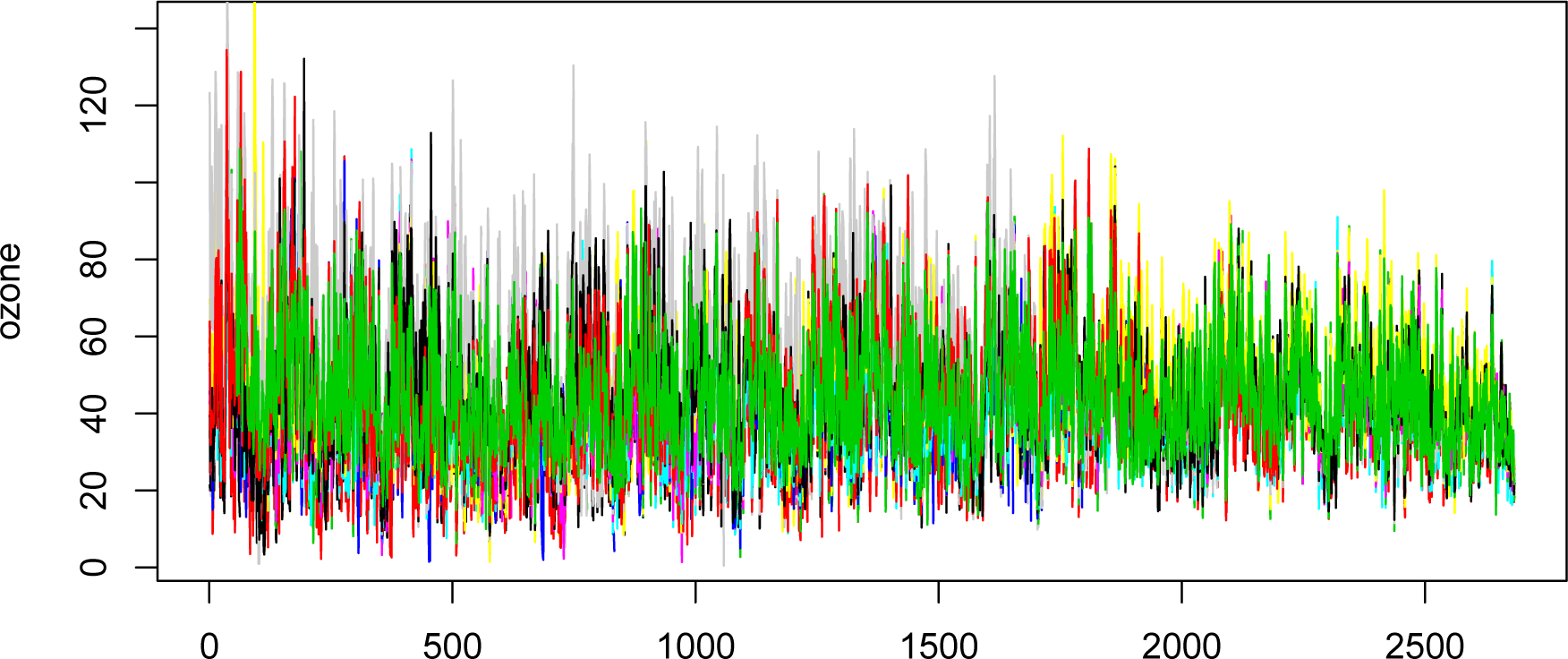
In this section, we use the methodology proposed in the previous section to detect changes in ground-level ozone concentration data collected in the Toronto region of Canada between June and September for the years from 1988 to 2009. There are 19 monitoring stations in this region, and the rate of missing data at each station is below 50%. We primarily focus on the daily time scale in four consecutive summer months from June to September for the years ranging from 1988 to 2009. Thus, we have the original data
Xi,t,
i = 1,…, 19;
t = 1,…, 2684, formed by 2684 (22 years × 122 days) daily maximum eight-hour moving averages of hourly ozone concentration data recorded in micrograms per cubic meter from each of the 19 stations, which are displayed in
Figure 1.
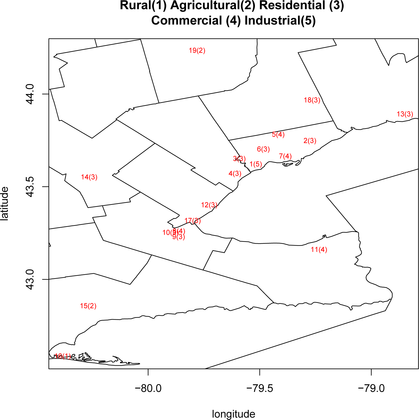
Figure 2 displays the locations of the 19 stations and their indexes. The numbers of missing data at nine of the stations are under 200, while the numbers of missing data at the other five stations are between 400 and 800. The remaining five stations have a number of missing data close to 1000.
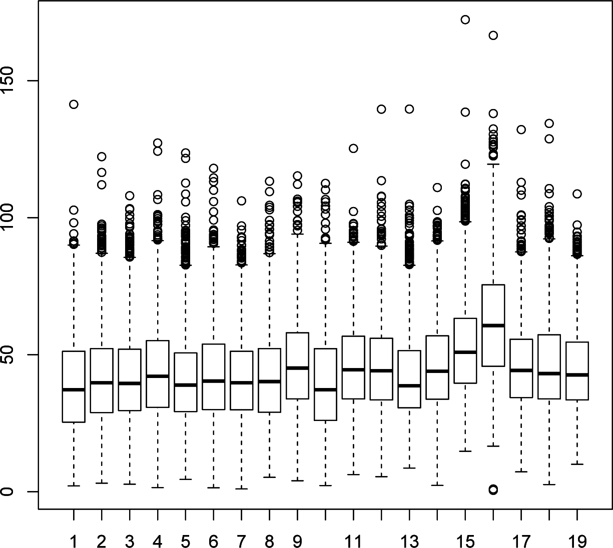
Figure 3 presents the box-and-whisker plots of the data collected at each station. It is clear that the data at each station are not normally distributed. Thus, we apply the Box–Cox power transformation
(1) to the data {
Xi,t} and obtain the transformed data {
Zi,t(λ)}, for each λ ∈ {0.3, 0.31, 0.32,⋯, 0.6}. The final value of λ will be decided later.
Since there are 122 days from 1 June to 31 September in each year, the time period is thus 122, so that
L in the model
(2) is 61. Preliminary data analysis shows that we may use the temporal model
(2) with
p = 1 and
q = 3 to fit the data. We write the model
(2) with
p = 1 and
q = 3 as follows:
Let λ ∈ {0.3, 0.31, 0.32,⋯, 0.6}. For each λ and a fixed
i, we fit the model
(7) to the data {
Zi,t(λ)} by least squares and obtain the estimates
,
j = 1,⋯, 5, of the parameters
βj,i(λ),
j = 1,⋯, 5. We compute the residuals
by:
We remark that the purpose of applying the Box–Cox power transformation to the ozone concentration data is such that {
εi,t(λ)} are approximately normally distributed. Thus, we can choose λ in terms of
p-values of a normality test on
for each fixed pair of λ and
i. In this application, the Pearson chi-squared test (R code: pearson.test) is employed. By applying this test to the residuals
for fixed λ and
i, we obtain the
p-value
pi(λ). Let
p(λ) = Median {
pi(λ),
i = 1,⋯, 19} for each λ ∈ {0.3, 0.31, 0.32,⋯, 0.6}.
is chosen, such that
, which turns out to be 0.48. Hence,
is used in the Box–Cox power transformation
(1) hereafter.
Let
As discussed above, {
Yi,t} for each fixed
i are modelled as:
where
t = 1,…,
T. As done previously, we estimate
βj,i,
j = 0, 1,…, 5 by the least squares method. Denote these estimates by
, 1,…, 5. We can then compute the residuals
for
t = 1,…,
T.
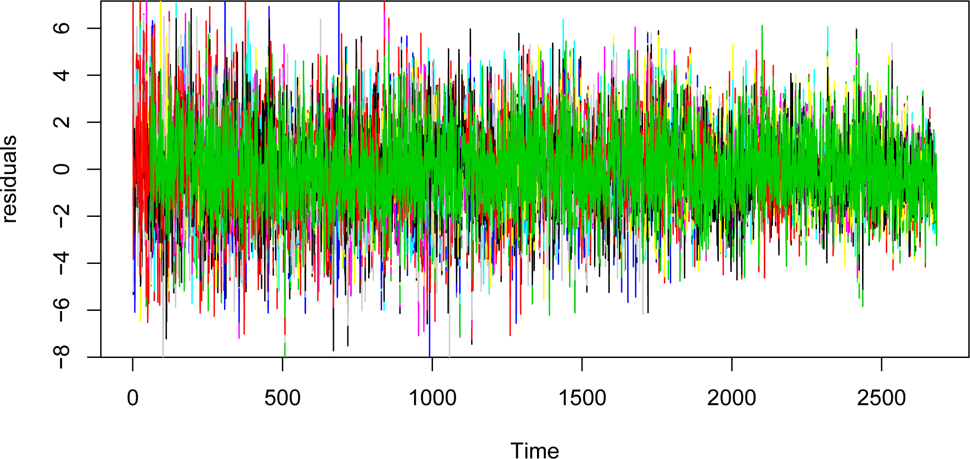
and
are plotted respectively in
Figures 4 and
5. To examine if the model has fitted the data from each station well, we compute
(the coefficient of determination) obtained by fitting the model
(8) to the data from each of 19 monitoring stations.
,
i = 1,…, 19 are displayed in
Table 1, which shows that the values of
are all larger than 0.95. We also compute the
p-value
pi obtained by performing Pearson chi-square test on
for
i = 1,…, 19, which are also displayed in
Table 1. From this table, it can be observed that only three
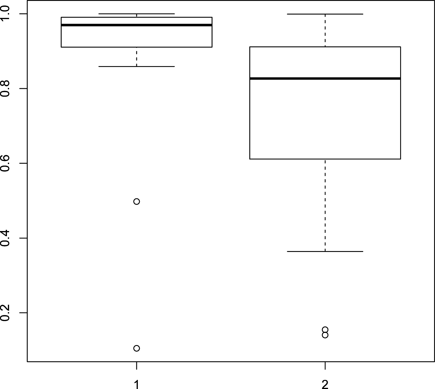
p-values of the Pearson chi-square test are smaller than 0.01. Further, for each time series
, we compute the Box–Pierce test statistic ([
23])for each of the two null hypotheses H
0 :
ρ(1) =
ρ(2) =
ρ(3) =
ρ(4) = 0 and
H0 :
ρ(1) =
ρ(2) = ⋯ =
ρ(7) = 0, where
ρ(
k) is the autocorrelation at lag
k (R code: Box.test). The box-and-whisker plot of the
p-values from the Box–Pierce test is displayed in
Figure 6, which shows that both null hypotheses cannot be rejected,
i.e., the residuals can be considered as uncorrelated at Lags 1 to 7.
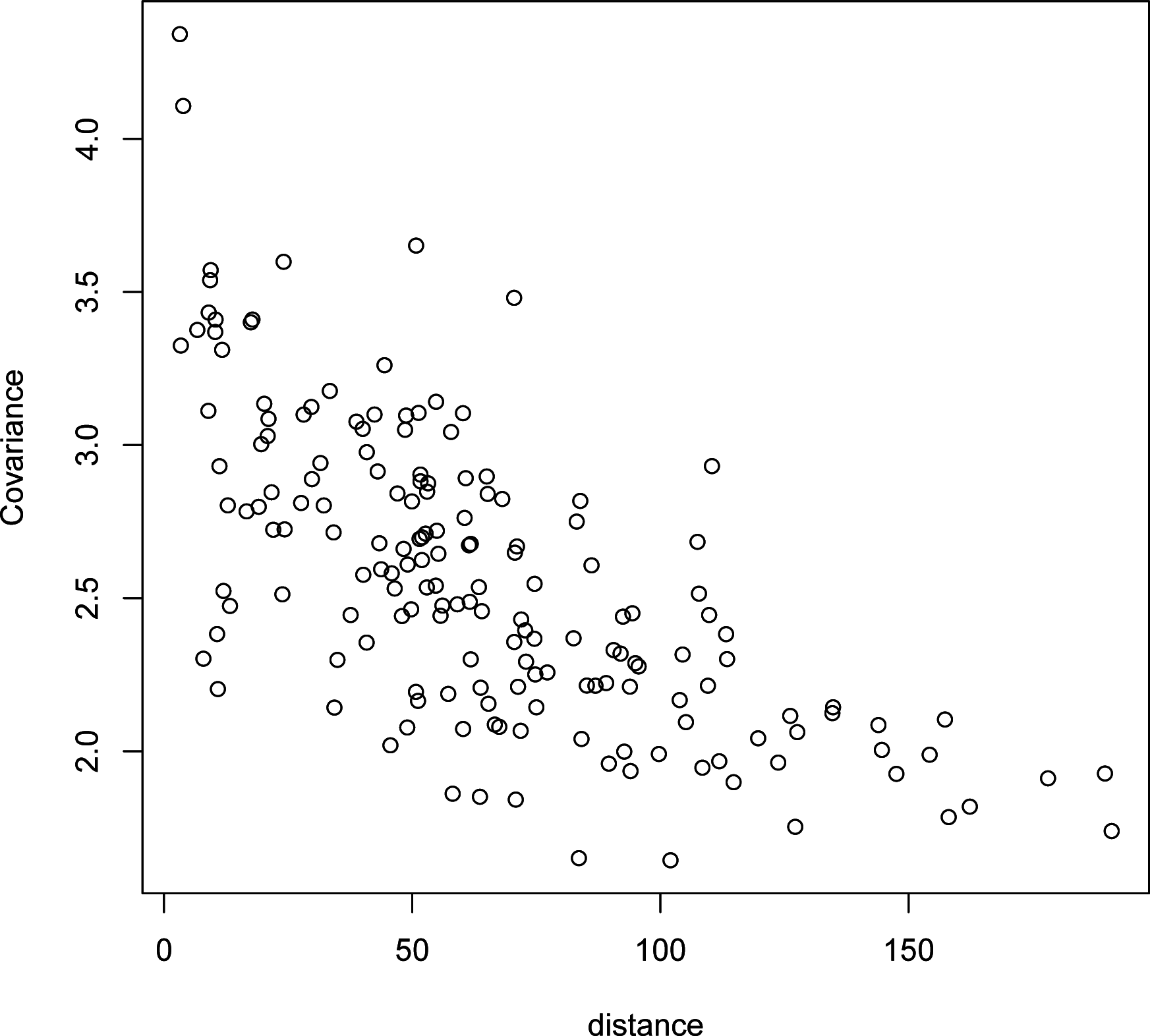
Let
.
Figure 7 displays the sample covariance
,
i,j = 1,…,19 and
i ≠
j, against the distance
, where (
si,1,
si,2) is the rectangular coordinate of the location of the
i-th station. It can be seen that the covariance decreases as the distance increases. Thus, we construct the spatial weight matrix
W = (
wi,j)
19×19 in
(3) by letting all of its diagonal elements {
wi,i} be zeros and off-diagonal elements {
wi,j,
i ≠
j} be the inverse distances between the stations
i and
j,
i.e.,
wi,j = 1/d
i,j.
The data have been assumed to be spatially correlated. To confirm this, Moran’s I is used to test the dependence at each time, which is computed by:
with
. More than 86% of the tests on the data at each time point are significant at the 0.05 level.
Replace
ε·t by
in Model
(3). By Ord (1975) [
18], we obtain the maximum likelihood estimates
and
of
(3), and then, we obtain the estimate of
. Thus, we obtain
, an estimate of the differential entropy defined in
(4).
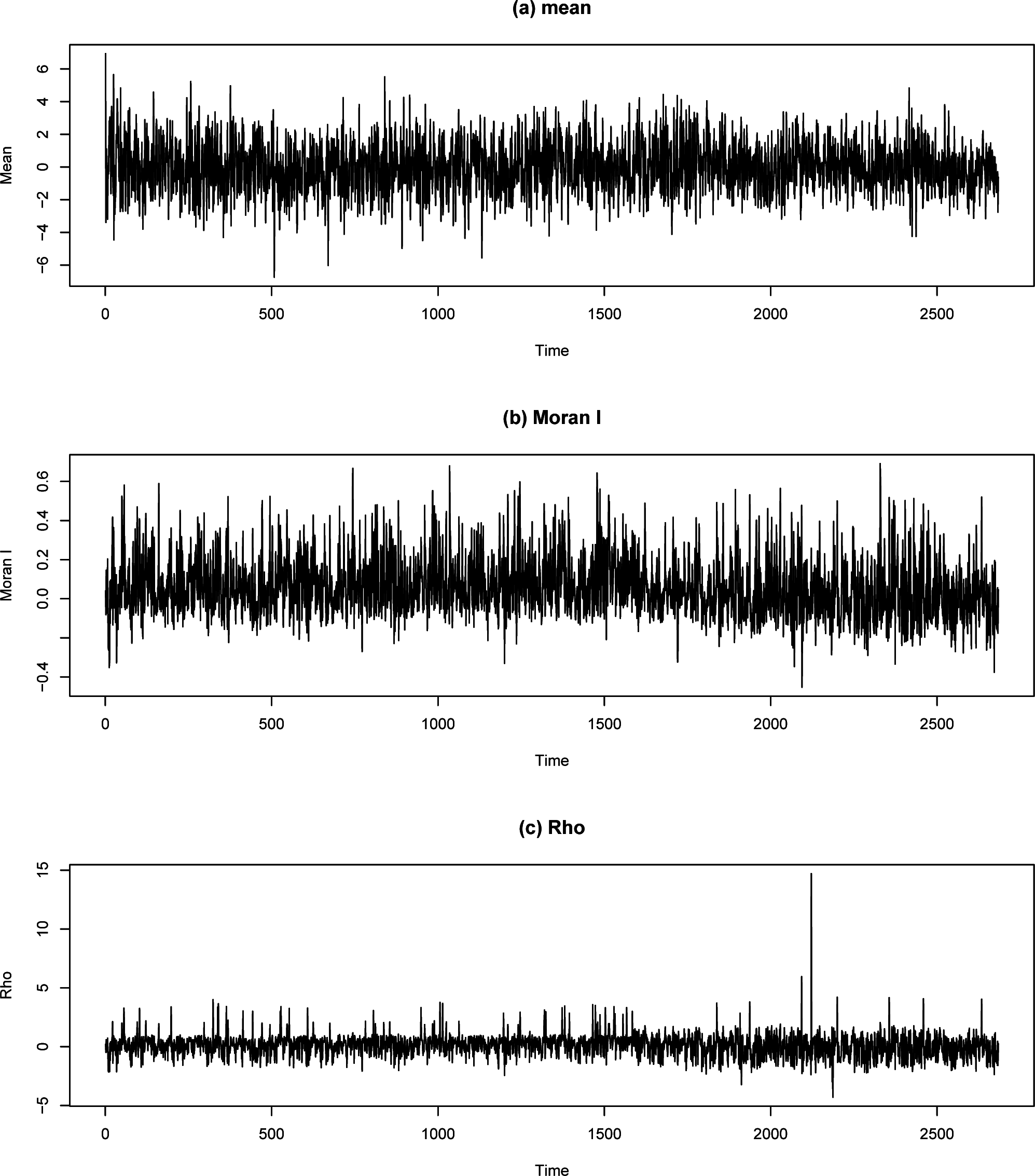
As shown in
Figure 6,
can be considered to be independent distributed, and the same argument is also true for
,
,
and {
ĥt}. Let
be the sample variance. The sample mean
, Moran’s I
and
are respectively displayed in
Figure 8. We apply the change-point detection method given in [
21] to each time series of
,
and
and cannot find any change-point. Thus, if we only consider the time series
,
and
, we have to claim that there is no change in the ozone concentration in the Toronto region. In contract, by applying the same method to both time series
and
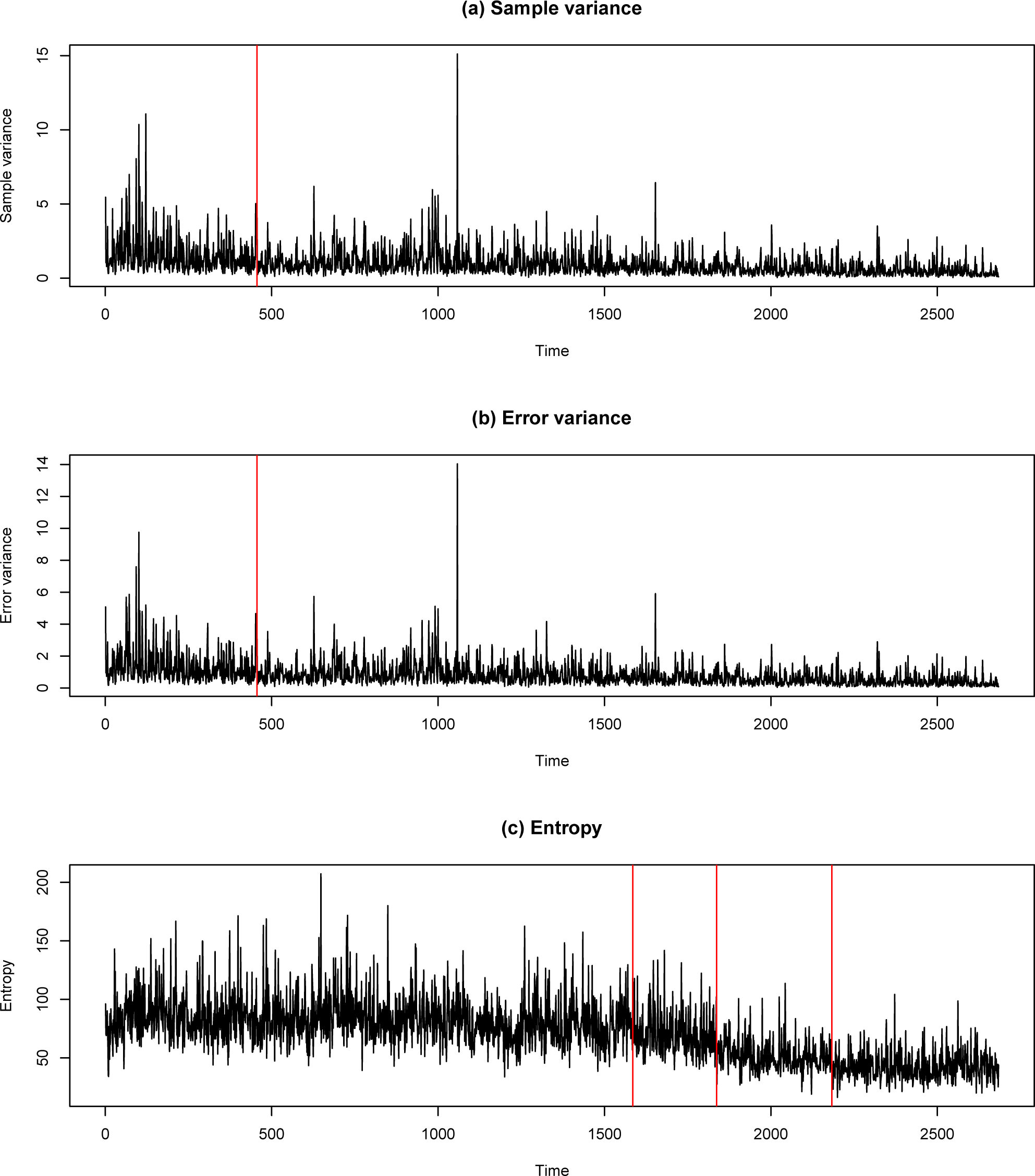
, we detect the same change-point at 456 (29 August 1991). If we also apply the same method to the time series {
ĥt}, we find three change-points, 1585 (30 September 2000), 1837 (7 June 2003) and 2183 (17 September 2005). The sample variance
, error variance
and entropy
ĥt are respectively displayed in
Figure 9.
By Simmons (2002) [
24], each year in Canada, 16,000 people die prematurely as a result of air pollution. Cars and light trucks are responsible for the majority of transportation emissions, but the heavy trucks in the trucking industry are also a major contributor, whose emissions have increased more rapidly than any other element of the Canadian transportation sector. Historically, Canada has taken a passive approach to the regulation of motor vehicle pollution. The estimated change-points, 1585 (30 September 2000), 1837 (7 June 2003) and 2183 (17 September 2005), are consistent with the following published regulations. By the 44th Working Party on Pollution and Energy (GRPE) of the United Nations [
25], since 1988, Canadian on-road vehicle emission standards have been, through a combination of regulations and voluntary agreements, aligned with those of the U.S. EPA (Environmental Protection Agency). The Canadian Environmental Protection Act 1999 transferred the responsibility to the Department of the Environment. Environment Canada adopted the Sulphur in Gasoline Regulations in June, 1999, and proposed the Sulphur in Diesel Fuel Regulations in December, 2001. The Canadian Department of the Environment (Environment Canada) published proposed new on-road vehicle and engine emission regulations on 30 March 2002. Regulations for each of the five off-road groups were proposed later in 2002 and during 2003. Sulphur in gasoline was limited to on average 30 parts per million (ppm) in 2005, with an interim limit of 150 parts per million in 2002. It is noted that ground level ozone is not emitted directly into the air, but is created by chemical reactions between oxides of nitrogen and volatile organic compounds, which include sulphur content. Thus, limiting sulphur in gasoline can help to improve the air quality.
4. Conclusion
In this paper, we propose a methodology for detecting changes in ground-level ozone concentrations by using entropy. It is shown via a real data example that the entropy ĥt, a function of
and
, can be used for detecting changes in ground-level ozone concentration data. As demonstrated in Section 3, when the same change-point detection method is applied to each of the time series
,
,
,
,
and {ĥt}, the time series that is the best for detection of multiple change-points is {ĥt}. This may be due to the fact that the entropy can be used to measure various spatial uncertainties, including both spatial variance and spatial dependence, and is able to extract more information from the data than some other statistics, e.g.,
and
. The proposed methodology is also applicable to other climate data.
As shown in the data example, the changes in both the mean and spatial dependence of ozone concentrations may not be detectable statistically after the regulations of environmental agencies are proposed. In contrast, the changes in the spatial uncertainties of ground-level ozone concentrations, measured by entropy, may be detectable statistically. Thus, after a regulation is promulgated, environmental agencies may be effective at monitoring the air quality change by employing the methodology presented in Section 2, which may help them to decide what is the next step for improving air quality.


