Abstract
Physical models and grey system models (GSMs) are commonly used to evaluate and predict physical behavior. A physical model avoids the incorrect trend series of a GSM, whereas a GSM avoids the assumptions and uncertainty of a physical model. A technique that combines the results of physical models and GSMs would make prediction more reasonable and reliable. This study proposes a fusion method for combining two trend series, calculated using two one-dimensional models, respectively, that uses a slope criterion and a distance weighting factor in the temporal and spatial domains. The independent one-dimensional evaluations are upgraded to a spatially and temporally connected two-dimensional distribution. The proposed technique was applied to a subsidence problem in Jhuoshuei River Alluvial Fan, Taiwan. The fusion results show dramatic decreases of subsidence quantity and rate compared to those estimated by the GSM. The subsidence behavior estimated using the proposed method is physically reasonable due to a convergent trend of subsidence under the assumption of constant discharge of groundwater. The technique proposed in this study can be used in fields that require a combination of two trend series from physical and nonphysical models.
1. Introduction
Subsidence is a worldwide hazard [–]. Commonly used methods for studying land subsidence include data analysis [–], physical calculation [–] and numerical simulation [–]. Data analysis analyzes the monitoring data, and prediction is mainly used for evaluating the type or trend of subsidence. The method used for prediction can be a black box model (e.g., regression analysis) or grey box model (e.g., grey system model (GSM)). Data analysis can avoid the assumptions in a physical model. However, the prediction results are easily affected by misleading monitoring data and the predicted series might deviate from physical behavior. Physical calculation uses experimental data, monitoring data of subsidence, or groundwater level data to determine subsidence using physics. The approach produces results that have physical support and are close to actual behavior. However, it is commonly used under a regular or simple conditions and uncertainty is introduced in the model assumptions and adopted parameters. Numerical simulation uses a physical theory to represent a complex situation. It is widely used in evaluating subsidence problems. Consolidation theory [] and poroelastic theory [] are commonly used physical theories for subsidence evaluation. A physical model avoids the incorrect behavior of a grey box model, whereas a grey box model avoids the assumptions and uncertainty of a physical model. Therefore, a technique that can fuse the results of physics-based and grey-box-based models would make the prediction of land subsidence more reasonable and reliable.
Subsidence monitoring is commonly a point type system, with the data obtained in the temporal domain for each point []. A one-dimensional model is thus commonly used for subsidence investigation due to its simplicity and convenience []. However, uncertainty is embedded between monitoring points in the spatial domain, and the spatial information of subsidence is lacking between the data points in a one-dimensional model. A multi-dimensional model can be used but it is more complex and time-consuming. A technique that can connect the one-dimensional points in the spatial domain would be useful. Previous studies on fusing different types of time series have focused on the temporal domain, with few considering the spatial domain [–]. The present study thus proposes a technique that can fuse two types of time series for subsidence prediction results in both the spatial and temporal domains.
Poroelastic theory, proposed by Biot [], is a rigorous physical theory for subsidence investigations [–,–]. This theory uses a coupled system that can solve soil deformation and pore water pressure at the same time and obtain the dynamic interaction between the variables []. Soil deformation can change the hydrogeological and mechanical properties and affect the evaluation of subsidence quantity [–]. Wang and Hsu’s model, which considers the deformation effect on porosity, hydraulic conductivity, and Young’s modulus, are simpler and more complete than that of Kim and Parizek []. The nonlinear poroelastic model (NPM) developed by Wang and Hsu [] has been used in subsidence estimation in Taiwan with good results [,]. The NPM is suitable for Taiwan subsidence problems and is thus adopted in this study to construct a physics-based subsidence model in Jhuoshuei River Alluvial Fan, Taiwan.
Grey system theory, proposed by Deng [],is a grey box model that is used to study uncertain systems or systems with incomplete data. The GSM can be used to evaluate land subsidence for which the data set is limited []. Wang et al. [] combined the GSM and NPM by using the technique proposed in this study to investigate the land subsidence problem in Tainan, Taiwan. The present study proposes a fusion technique and shows the difference between the results with and without fusion in a subsidence evaluation of Jhuoshuei River Alluvial Fan, Taiwan. The fusion method combines the advantages of physics-based and grey-box-based models and fuses the one-dimensional predicted subsidence results in the spatial and temporal domains. The independent one-dimensional evaluations are then upgraded to a spatially and temporally correlative two-dimensional distribution.
2. Study Background
2.1. Study Area
Jhuoshuei River Alluvial Fan, located in central Taiwan (see Figure 1), is the largest alluvial fan in Taiwan. Wu River and Beigang River flow through the north and south areas, respectively, and Jhuoshuei River flows across the middle of the alluvial fan. Changhua and Yunlin Counties are located in the north and south divisions of Jhuoshuei River Alluvial Fan, respectively. The western boundary is the Taiwan Strait and the eastern boundary is Bagua and Douliu foothills, which are the main areas for groundwater recharge.
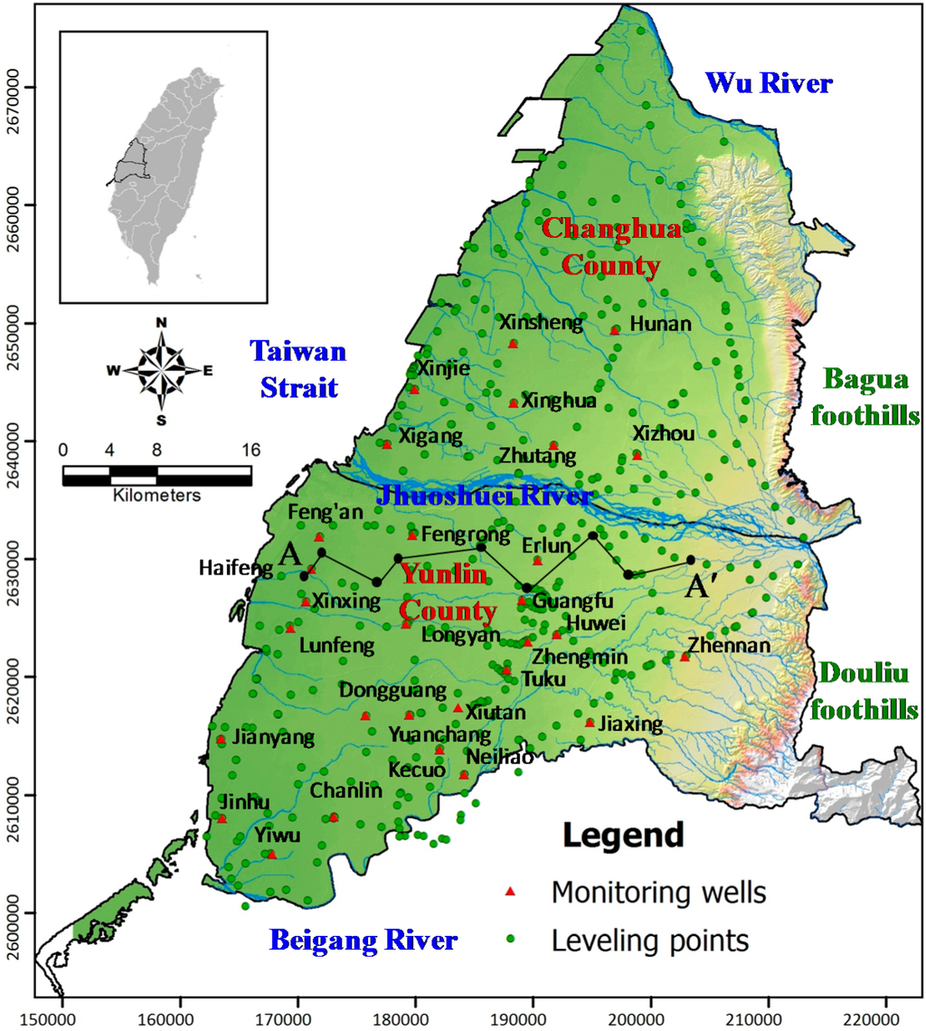
Figure 1.
Study area of Jhuoshuei River Alluvial Fan, Taiwan, and distribution of leveling points and multi-level compaction monitoring wells. A–A’ is the line representing the hydrogeological profile shown in Figure 2.
The Taiwan Water Resources Agency executed 93 hydrogeological drillings and setup 70 groundwater monitoring stations with 188 monitoring wells at various depths to investigate the groundwater resources in Jhuoshuei River Alluvial Fan []. Each groundwater station includes one to five monitoring wells at different depths. The distance between each well is about 5 km. The sampling frequency for groundwater level monitoring is one hour. One of the hydrogeoloical profiles is shown in Figure 2. The hydrogeology formations can be separated into seven units within a depth of 300 m. They are referred to as aquifer one, aquitard one, aquifer two, aquitard two, aquifer three, aquitard three and aquifer four. The layer system is obvious in the mid and tail fans but not obvious in the top fan due to its composite material being mostly gravel. The aquifers thin out beneath the Taiwan Strait and stretch from the tail fan. Detailed hydrogeological descriptions can be found elsewhere [,].
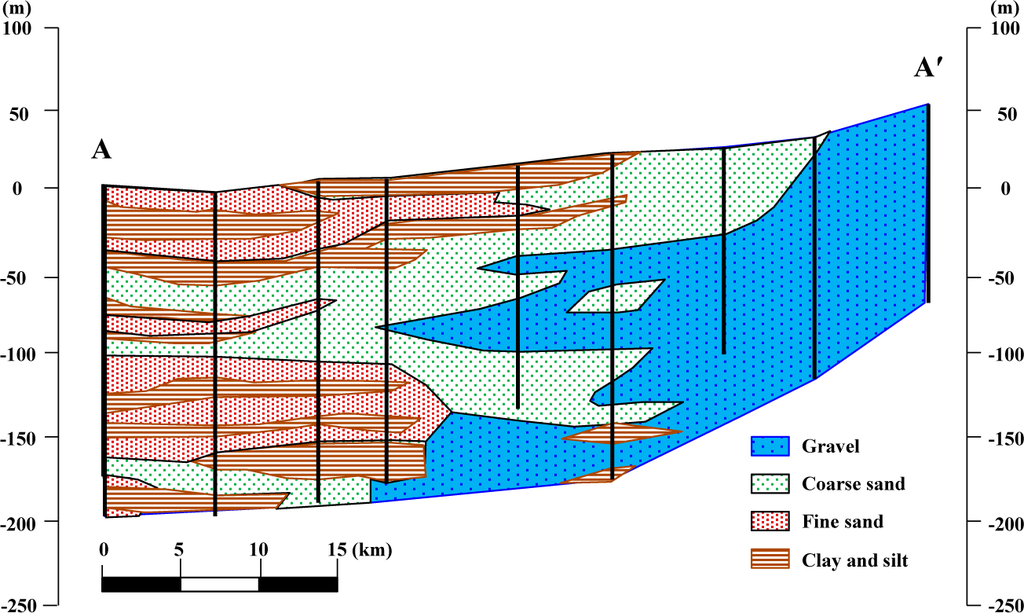
Figure 2.
One hydrogeological profile of Jhuoshuei River Alluvial Fan, Taiwan. The profile trace is shown in Figure 1.
Jhuoshuei River Alluvial Fan contains a great amount of groundwater. However, there is little surface water in this area due to industrialization and urbanization. Groundwater is thus mainlyover-pumped for public, irrigation and industrial usage, which has induced subsidence. According to an investigation by the Taiwan Water Resource Agency, there are about 182,000 wells in Jhuoshuei River Alluvial Fan, with a total pumping quantity of around 2.16 billion m3/year [,]. The maximum subsidence rate is 6.1 cm/year and the continuous subsidence area (subsidence rate larger than 3.0 cm/year) was about 309.1 km2 in 2014 []. Taiwan High Speed Rail passes across the subsidence areas, which is a safety concern []. Subsidence in Jhuoshuei River Alluvial Fan is thus an important issue for the Taiwanese government.
2.2. Subsidence Monitoring
Four types of monitoring systems are used in Taiwan for subsidence investigation, namely leveling, Global Positioning System (GPS), multi-level compaction monitoring wells (MCMWs), and interferometry synthetic aperture radar (InSAR). Leveling and MCMW data are adopted in this study due to their relatively long monitoring periods. MCMW data provide compaction information at various depths, and the experimental data from the wells provide the physical properties. MCMW data are suitable for the study of NPMs. Leveling monitoring has been used for a long period for subsidence observation in Taiwan. The monitoring density is high and can compensate for the lack of MCMWs. The leveling data are suitable for GSMs. Detailed descriptions of the monitoring system can be found elsewhere [].
There were 29 MCMWs and 708 leveling points in 2011 in Jhuoshuei River Alluvial Fan, Taiwan, as shown in Figure 1. The measurement frequencies are monthly for the MCMWs and yearly for leveling in this area. The land subsidence data from 2007 to 2011 are adopted, and thus the subsidence quantities shown in this study are relative to the level in 2007. Only 26 MCMWs and 452 leveling points are used in this study due to a lack of monitoring data. The basic information for the 26 MCMWs is listed in Table 1. The monitoring depth is 200 to 330 m. The earliest installed monitoring wells are Haifeng, Lunfeng, Jianyang and Jinhu wells, which were installed in December 1994 at a depth of 200 m. Three recently installed wells (in August 2009), namely Dongguang, Yiwu and Zhengmin wells, are not adopted in this study due to their short monitoring period. Zhengmin well has the largest monitoring depth (=330 m).

Table 1.
Basic information for multi-level compaction monitoring wells (MCMWs) adopted in this study.
From the 26 monitoring wells, the subsidence quantity at the ground surface is the largest at Yuanchang well (= 0.252 m) and the smallest is at Jiaxing well (=0 m) in 2011 based on 2007. However, the compaction quantity at different depths can be different. Figure 3 shows the monitoring data for two of the MCMWs as anillustration. Figure 3a shows the compaction in the spatial domain at various periods at Xinghua well, which has the largest land subsidence quantity in Changhua County. The slope of the curve represents the compaction rate. Therefore, the main compacted formation in 2011 is at about 100–250 m, contributing 80% of total land subsidence. Figure 3b shows the compaction at various depths at Yuanchang well, which has the largest land subsidence quantity in Yunlin County. The compaction at different depths of Yuanchang well is more uniform than that of Xinghua well. The main compacted formation in 2011 was at about 50–280 m, contributing 89% of total land subsidence.
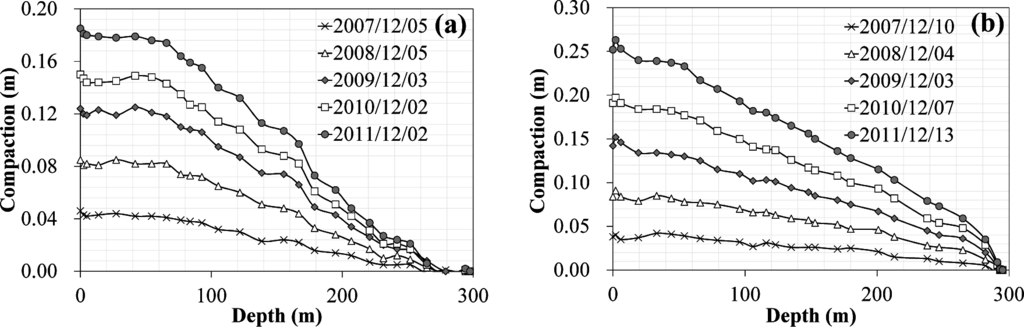
Figure 3.
Monitoring data from MCMWs at (a) Xinghua and (b) Yuanchang wells in spatial domain at various periods.
3. Methodology
3.1. Nonlinear Poroelastic Model
The nonlinear poroelastic model (NPM) was developed by Wang and Hsu []. The governing equations for the one-dimensional poroelastic model can be written as []:
where w is the vertical displacement; P is the change in pore water pressure; z is the vertical direction; t is time; a is called the final compressibility with a−1 = λ + 2µ, where λ and µ are Lame’s constants (µ = E/2(1 + v), and λ = Ev/(1 + v)(1 − 2v), where E is Young’s modulus, and v is Poisson’s ratio); a is the dimensionless coefficient of the effective stress; Q−1 is the compressibility introduced by Biot; and κ is the Darcy conductivity, which is related to hydraulic conductivity K by K = λwκ, where λw is the unit weight of water (= 9810 N/m3).
Following Wang and Hsu [], the porosity (n), hydraulic conductivity (K), and Young’s modulus (E) under the deformation effect can be written, respectively, as:
where ε is the volume strain, and the subscripts 0 and 1 indicate before and after the deformation effect, respectively. The nonlinear parameters are embedded in the calculation during the modeling period.
3.2. Grey System Model
The GSM is based on the eigenvalue system and the model established based on the grey prediction theory. During the grey simulation, the accumulated generating operation is applied to the discrete and irregular initial number series to make the series generate an exponential rule, based on which the grey differential equation is established. The GSM can be established using data preprocessing and the grey differential equation. Generally, a method based on the time series model is used to process irregular data in order to smooth the series and increase prediction precision.
The leveling data are limited due to the sampling rate being yearly in Jhuoshuei River Alluvial Fan, Taiwan, and the measurement points being different in each year. Most of the leveling data have only four subsidence measurement points in the temporal domain. Therefore, the GSM is a suitable model for subsidence prediction with the use of leveling data.
Deng [] proposed the grey system prediction theory. The GSM with one first-order variable is called the GM (1,1) model. The grey differential equation of the GM (1,1) model can be written as:
where a and b are coefficients often evaluated using the least squares error method by fitting the theory and observation data and x(1) is a canonical series written as:
where x(0) is the original data series (i.e., leveling data series in this study) and N is the data number. Substituting the evaluated a and b into Equation (5) and letting the initial condition be x(1)(1) = x(0)(1) yields:
where
is the predicted value for x(1) at the n + 1 point. Using back differential for
yields:
The predicted value
is thus obtained. Equation (8) is the basic equation for the GM (1,1) model.
The GSM developed by Hung et al. [] is used to construct a GM (1,1) grey prediction model of subsidence in this study. Four data points of a leveling time series are input into the GSM model, and then the point for the next time step is predicted. Considering the time interval and subsidence quantity of the leveling data, the subsidence time series is evaluated by the GSM at each leveling point, as shown in Figure 1. After the subsidence time series for all the leveling points have been evaluated, the results of the GSM are obtained.
3.3. Model Settings
Land subsidence is mainly caused by surface loading and groundwater pumping. Considering both the mechanism of top loading and aquifer pumping, the conceptual model for a one-dimensional column is proposed []. The quantities of top loading and bottom discharge are evaluated by fitting the results of the NPM to the monitoring data. The adopted parameters for the NPM are listed in Table 2. The property at each MCMW in this study is assumed to be homogeneous in the vertical direction with the mean value of the parameters. The mean porosity and hydraulic conductivity are obtained from triaxial permeability tests. The Young’s modulus and Poisson’s ratio are taken from Das []. However, since some MCMWs do not have experimental data, mean values from the other MCMWs were used in the model.
Table 2.
Adopted parameters in nonlinear poroelastic model (NPM).
The settings of the NPM are similar to those in Wang et al. [] except for the adopted parameters, and those of the GSM are the same as those in Wang et al. [] except for the monitoring data. Detailed descriptions of the NPM and the GSM for subsidence evaluation can be found elsewhere [,].
3.4. Fusion Method
The subsidence predicted using the GSM shows a continuous increasing (or decreasing) trend due to the use of monitoring data from leveling, whereas that predicted using the NPM shows a convergence trend due to physical behavior. Based on the physical mechanism, the subsidence rate should decrease and tend to be stable if the driving force is constant. Therefore, the converging results of the NPM are reasonable, and thus the slopes in each time step of the convergent curve are adopted for the combination. The subsidence predicted using the GSM follows the monitoring data. The subsidence quantities in the initial period evaluated by the GSM should be reliable and are thus adopted for the combination. The number of leveling points is larger than the number of MCMWs in Jhuoshuei River Alluvial Fan, Taiwan. The fusion results thus can provide a better estimation than using each of the models.
The fusion concept is to use the results of the NPM to re-evaluate the results of the GSM under a slope criterion of the subsidence trend in the temporal domain and a weighting factor between the monitoring points in the spatial domain. Figure 4 shows a schematic map of the distribution of monitoring points (one for the GSM and three for the NPM). The distances from GSM1 to NPM1, NPM2, and NPM3 are d11, d12, and d13, respectively (i.e., dij is the distance from GSMi to NPMj). The slopes of the subsidence trend for GSMi and NPMj between time t and t −1 can be written, respectively, as:
where GSMi and NPMj are the evaluated subsidence values for the GSM at position i and the NPM at position j, respectively.
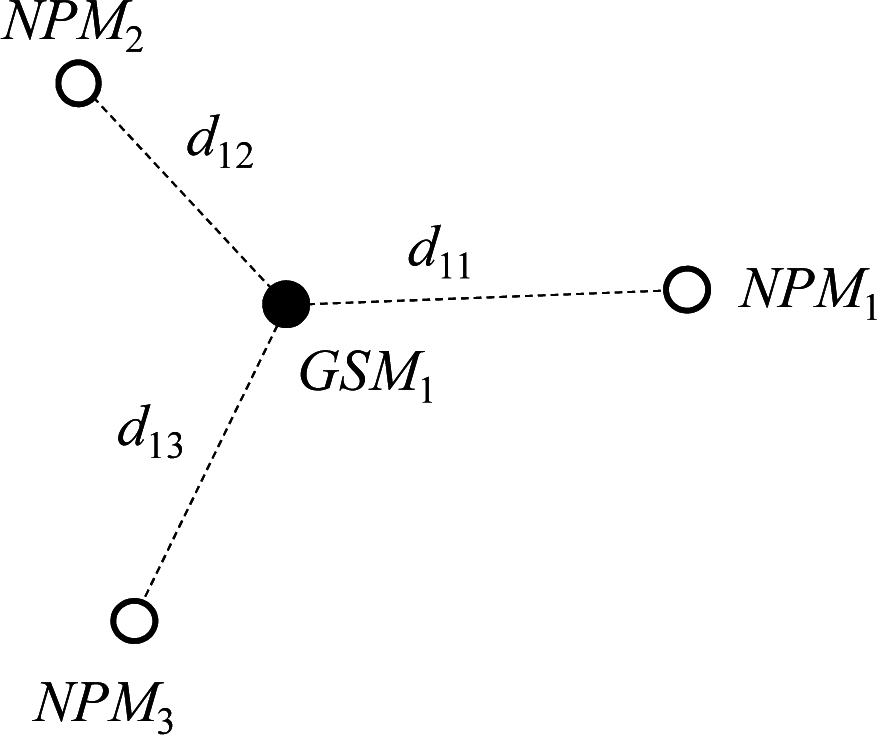
Figure 4.
Schematic map of distribution of monitoring points. Grey system models (GSM)i and NPMj indicate monitoring points for grey system and poroelastic models, respectively. d11, d12, and d13 are distances from GSM1 to NPM1, NPM2, and NPM3, respectively.
Considering a distance weighting factor between the locations of GSMi and NPMj, the mean slope of the subsidence trend for NPMj with respect to GSMi can be written as:
where
is the mean slope of NPMj with respect to GSMi in the time interval dt and m is the number of monitoring points for the NPM (i.e., the number of MCMWs). A distance weighting between the points for the GSM and the NPM is considered in calculating the mean slope of the NPM. The influence decreases with increasing distance between the GSM and the NPM.
It is assumed that the subsidence trends obtained from the results of the NPM and the initial subsidence quantities obtained from the results of the GSM are correct. The initial subsidence quantity of the GSM is kept but the slope of the subsidence trend obtained from the GSM is adjusted using the slope calculated from the NPM. If the slope of the subsidence trend obtained from GSMi in the time interval dt is larger than the mean slope of NPMj in the same time interval, the slope of GSMi is substituted by the mean slope of NPMj. The slope criterion can be written as:
The slope criterion is used to evaluate the slope of the subsidence trend in each time interval for each leveling point with respect to all MCMWs by considering the distance weighting factor. Both the spatial and temporal results are combined in the fusion technique. The independent one-dimensional evaluations in the NPM and the GSM are then upgraded to a spatially and temporally relative two-dimensional distribution.
4. Results and Discussion
4.1. Results for Nonlinear Poroelastic Model
The MCMWs with maximum and minimum subsidence in Changhua and Yunlin, respectively, are chosen as examples for illustrating the fitting situation, as shown in Figure 5. The Xinghua and Xizhou MCMWs are in Changhua County and the Yunchang and Jiaxing MCMWs are in Yunlin County. The land subsidence in these four MCMWs shows a continuous increasing trend and fluctuation, which is due to the recurrent dry and wet seasons. The subsidence fluctuation is more dominant in Yunlin County (Figure 5c,d) than in Changhau County (Figure 5a,b) due to the large fluctuation of groundwater level in Yunlin County. The fitting for Jiaxing well is poor due to the negative subsidence and the adopted compaction NPM, as shown in Figure 5d. Negative subsidence indicates an uplift situation, which is not considered in the NPM in this study. From the data trend of Jiaxing well, the original land surface should be lower than the initial monitoring data in May 2008. The large fluctuation of the monitored land subsidence and the lack of the original land surface has led to the negative subsidence situation. If the original land surface can be found, the poor fitting situation can be improved.
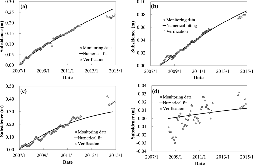
Figure 5.
Four MCMWs for demonstrating fitting results. (a) Xinghua; (b)Xizhou; (c) Yunchang; and (d) Jiaxing wells. White triangles show data used for model verification.
From the results of the NPM, the subsidence trend in the calibration period shows both convergence and divergence. However, the land subsidence approaches an asymptotic value for a long period due to the constant driving forces. Based on physical behavior, subsidence should converge under a constant driving force in the steady-state condition.
The verification results of the NPM are shown in Figure 5. The subsidence data for 2012–2014 are adopted for model verification. However, the data from March 2012 to March 2014 are missing due to an equipment operation error. From the verification results in Figure 5, the subsidence predicted using the NPM in Changhau County shows an overestimated pattern (Figure 5a,b) and that in Yunlin County shows an underestimated pattern (Figure 5c,d). The verification results are consistent with the monitoring results, which showed that land subsidence (groundwater level) in Changhua is decreasing (increasing) and that in Yunlin is still increasing (decreasing) []. Therefore, the predicted subsidence in the following section might be overestimated in Changhua County and underestimated in Yunlin County.
The best fits for the subsidence data from the MCMWs and the numerical results from the NPM are listed in Table 3. The fitting R2 values are good for the MCMWs except for the Jiaxing well. The reason for the poor fitting has been mentioned previously and is shown in Figure 5d. From the fitting results, the quantity of discharge is 0 to 2.58 × 10⁻⁹m/s and that of loading is 0 to 1.07 × 10⁴ N/m2. Two and 15 MCMWs show zero discharge and zero loading, respectively. The main driving force for the land subsidence in Jhuoshuei River Alluvial Fan is groundwater pumping, which is expressed as discharge (pumping rate in unit area) in Table 3. The influence of top loading is relatively small, occurring only at 11 MCMWs. The quantities of loading are also small, lower than atmospheric pressure (= 1.013 × 10⁵ N/m2).
Table 3.
Calibration results for NPM at MCMWs.
4.2. Results for Grey System Model
The predicted subsidence of the GSM was calculated time period by time period and point by point. The predicted subsidence distribution in 2039 is shown in Figure 6, as obtained by applying the interpolation method. The main land subsidence areas are located in the central areas of Yunlin and Changhua Counties. The pattern is similar to that of the monitoring data (not shown here) due to the nearly linear increment of the GSM. The maximum subsidence estimated using the GSM (2.31 m) occurs in Yunlin County. The maximum subsidence rate is 7.4 cm/year, which is larger than the rate for serious hazard potential of subsidence (5.0 cm/year) [].
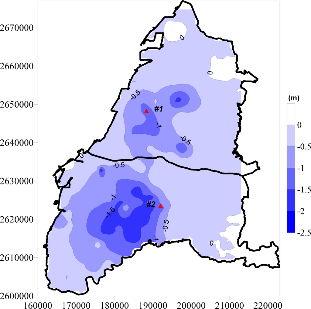
Figure 6.
Subsidence distribution in Jhuoshuei River Alluvial Fan in 2039 obtained using GSM. Triangle symbols numbered #1 and #2 are locations of demonstration points used for fusion results in Figure 8.
A relatively large subsidence for 2039 is obtained using the GSM due to the linear increasing trend of the monitoring data. Based on physical behavior, soil consolidation has a convergence trend if the exerted stress and/or pore water pressure changes are constant. A linear increasing subsidence trend is thus unreasonable under an unchanging driving force. Therefore, the predicted subsidence quantities shown in Figure 6 are overestimated. The fusion technique is thus applied to combine the two subsidence trend series from the NPM and the GSM in the spatial and temporal domains to obtain a reasonable and reliable estimation.
4.3. Subsidence Fusion Results
The slope criterion for the subsidence trend series (Equation (12)) is adopted to re-calculate the results of the GSM by considering the mean slope calculated from the NPM with a distance weighting factor. The fusion results for subsidence distribution in Jhuoshuei River Alluvial Fan for 2039 are shown in Figure 7. Note that the subsidence distribution in Figure 7 is not an interpolated result but the fusion result. The pattern of the subsidence distribution is slightly different from that in Figure 6 but the quantity has dramatically decreased. The maximum subsidence decreases from 2.31 m to 0.59 m. The areas with subsidence quantities larger than 0.3 m are mainly located in the southwest areas of Changhua County and south-central areas of Yunlin County.
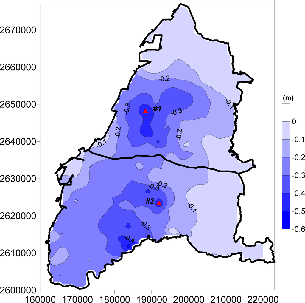
Figure 7.
Subsidence distribution with fusion in Jhuoshuei River Alluvial Fan in 2039 obtained using NPM and GSM. Triangle symbols numbered #1 and #2 are locations of demonstration points used for fusion results in Figure 8.
Comparisons of the results obtained with and without fusion for two leveling points are shown in Figure 8. The locations of the two leveling points are marked in Figures 6 and 7. The subsidence predicted using the GSM for the leveling points shows a linear increasing trend. The subsidence quantities for Points #1 and #2 are 0.71 and 1.23 m, respectively, for 2039. After using the fusion technique, both subsidence curves show convergence trends. The subsidence quantities are 0.55 and 0.53 m, respectively, and the differences are 0.16 and 0.70 m, respectively. The decreases vary with leveling point. The maximum subsidence is 0.59 m and the maximum subsidence rate is 1.0 cm/year for 2039. The subsidence behavior becomes reasonable for both the subsidence quantity and subsidence rate. Note that the subsidence trend for Fusion #2 in Figure 8 still increases with time. This fusion result indicates that the cumulative subsidence in Jhuoshuei River Alluvial Fan will increase in some areas after 2039 but will converge in the future, due to the application of physical theory.
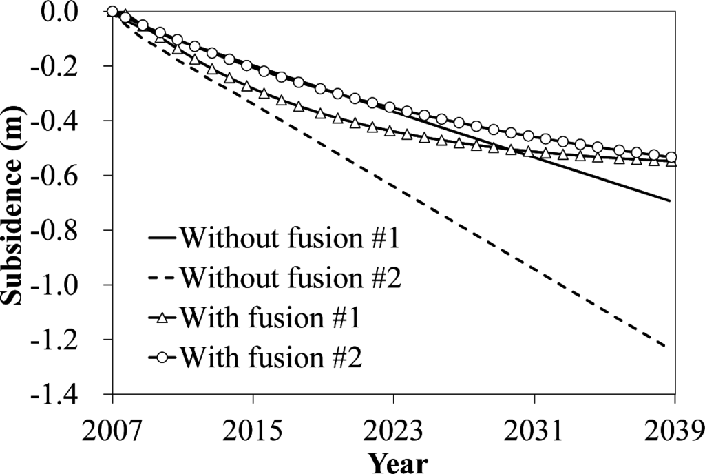
Figure 8.
Comparison of results obtained with and without fusion for two leveling points marked in Figure 7.
The subsidence predictions in this study include some assumptions and uncertainties. A one-dimensional NPM is adopted and lateral deformation is not considered in the estimation, which might have an influence on the predicted subsidence quantities. The adopted parameters were from laboratory tests and a previous study and thus might not represent the behavior in the field. The subsidence monitoring data may also have measurement errors. Further investigations are required for better estimation of land subsidence. Nevertheless, although the proposed subsidence models have their limitations and disadvantages, the fusion method can still work. The defects of the subsidence models do not affect the use of the proposed fusion technique. An improved fusion result can be obtained after the predicted subsidence results from the models being improved.
5. Conclusions
This study proposed a technique that fuses two trend series in the spatial and temporal domains using a slope criterion and a distance weighting factor and then applied it to investigate subsidence in Jhuoshuei River Alluvial Fan, Taiwan. The linear increasing trend of subsidence predicted using a grey-box-based GSM was corrected to a convergence trend with a physics-based poroelastic model. The fusion results show dramatic decreases of subsidence quantity and subsidence rate. The maximum subsidence quantity decreased from 2.31 to 0.59 m and the subsidence rate decreased from 7.4 to 1.0 cm/year for 2039. The subsidence behavior became physically reasonable for both the subsidence quantity and subsidence rate due to the convergence trend of subsidence under the assumption of constant discharge of groundwater and top loading. The proposed fusion technique upgrades the independent one-dimensional evaluations to a spatially and temporally connected two-dimensional distribution. The proposed method can also improve the subsidence distribution prediction when there are few subsidence monitoring wells. The proposed fusion method can be used for areas that require a combination of trend series in the spatial and temporal domains.
Acknowledgments
The author would like to thank the Taiwan Water Resources Agency and the Industrial Technology Research Institute for providing the subsidence monitoring data and experimental data, respectively. This study was supported by the Water Resources Agency, Taiwan, under grants MOEAWRA1010295 and MOEAWRA1010216 and the National Science Council, Taiwan, under grant NSC 101-2221-E006-194-MY3.
Conflicts of Interest
The author declares no conflict of interest.
References
- Bell, F. Engineering Geology, 2nd ed; Butterworth-Heinemann: Oxford, UK, 2007. [Google Scholar]
- Chen, Z.; Rybczyk, J. Coastal Subsidence. In Encyclopedia of Coastal Science; Schwartz, M., Ed.; Kluwer Academic Publishers: Dordrecht, The Netherlands, 2005. [Google Scholar]
- Galloway, D.; Burbey, T. Review: Regional land subsidence accompanying groundwater extraction. Hydrogeol. J 2011, 19, 1459–1486. [Google Scholar]
- Galloway, D.L.; Jones, D.R.; Ingebritsen, S.E. Land Subsidence in the United States: US Geological Survey Circular 1182; U.S. Department of the Interior, U.S. Geological Survey: Washington, DC, USA, 1999. [Google Scholar]
- Bell, J.W.; Amelung, F.; Ramelli, A.R.; Blewitt, G. Land subsidence in Las Vegas, Nevada, 1935–2000: New geodetic data show evolution, revised spatial patterns, and reduced rates. Environ. Eng. Geosci 2002, 8, 155–174. [Google Scholar]
- Bock, Y.; Wdowinski, S.; Ferretti, A.; Novali, F.; Fumagalli, A. Recent subsidence of the Venice Lagoon from continuous GPS and Interferometric Synthetic Aperture Radar. Geochem. Geophys. Geosyst 2012, 13, 1–13. [Google Scholar]
- Galloway, D.; Jones, D.R.; Ingebritsen, S. Measuring Land Subsidence from Space; USGS Fact Sheet-051-00; US Department of the Interior, US Geological Survey: Washington, DC, USA, 2000. [Google Scholar]
- Hung, W.C.; Hwang, C.W.; Chang, C.P.; Yen, J.Y.; Liu, C.H.; Yang, W.H. Monitoring severe aquifer-system compaction and land subsidence in Taiwan using multiple sensors: Yunlin, the southern Choushui River Alluvial Fan. Environ. Earth Sci 2010, 59, 1535–1548. [Google Scholar]
- Jambrik, R. Analysis of water level and land subsidence data from thorez open-pit mine, Hungary. Mine Water Environ 1995, 14, 13–22. [Google Scholar]
- Liu, B.; Dai, W.; Peng, W.; Meng, X. Spatio-temporal analysis of the land subsidence in the UK using Independent Component Analysis. Proceedings of the 2014 3rd International Workshop on Earth Observation and Remote Sensing Applications, Changsha, China, 11–14 June 2014.
- Asadi, A.; Shahriar, K.; Goshtasbi, K.; Najm, K. Development of a new mathematical model for prediction of surface subsidence due to inclined coal-seam mining. J. S. Afr. Inst. Min. Metall 2005, 105, 15–20. [Google Scholar]
- Cui, X.; Miao, X.; Wang, J.; Yang, S.; Liu, H.; Hu, X. Improved prediction of differential subsidence caused by underground mining. Int. J. Rock Mech. Min. Sci 2000, 37, 615–627. [Google Scholar]
- Dai, H.; Wang, J.; Cai, M.; Wu, L.; Guo, Z. Seam dip angle based mining subsidence model and its application. Int. J. Rock Mech. Min. Sci 2002, 39, 115–123. [Google Scholar]
- Donnelly, L.J.; de la Cruz, H.; Asmar, I.; Zapata, O.; Perez, J.D. The monitoring and prediction of mining subsidence in the Amaga, Angelopolis, Venecia and Bolombolo Regions, Antioquia, Colombia. Eng. Geol 2001, 59, 103–114. [Google Scholar]
- Rodriguez, R.; Torano, J. Hypothesis of the multiple subsidence trough related to very steep and vertical coal seams and its prediction through profile function. Geotech. Geol. Eng 2000, 18, 289–311. [Google Scholar]
- Ferronato, M.; Gambolati, G.; Janna, C.; Teatini, P. Numerical modelling of regional faults in land subsidence prediction above gas/oil reservoirs. Int. J. Numer. Anal. Methods Geomech 2008, 32, 633–657. [Google Scholar]
- Ferronato, M.; Gambolati, G.; Teatini, P.; Bau, D. Stochastic poromechanical modeling of anthropogenic land subsidence. Int. J. Solids Struct 2006, 43, 3324–3336. [Google Scholar]
- Gambolati, G.; Ricceri, G.; Bertoni, W.; Brighenti, G.; Vuillermin, E. Mathematical simulation of the subsidence of Ravenna. Water Resour. Res 1991, 27, 2899–2918. [Google Scholar]
- Gambolati, G.; Teatini, P.; Bau, D.; Ferronato, M. Importance of poroelastic coupling in dynamically active aquifers of the Po river basin, Italy. Water Resour. Res 2000, 36, 2443–2459. [Google Scholar]
- Hoffmann, J.; Galloway, D.; Zebker, H. Inverse modeling of interbed storage parameters using land subsidence observations, Antelope Valley, California. Water Resour. Res 2003, 39. [Google Scholar] [CrossRef]
- Hung, W.C.; Hwang, C.W.; Liou, J.C.; Lin, Y.S.; Yang, H.L. Modeling aquifer-system compaction and predicting land subsidence in central Taiwan. Eng. Geol 2012, 147–148, 78–90. [Google Scholar]
- Teatini, P.; Ferronato, M.; Gambolati, G.; Gonella, M. Groundwater pumping and land subsidence in the Emilia-Romagna coastland, Italy: Modeling the past occurrence and the future trend. Water Resour. Res 2006, 42. [Google Scholar] [CrossRef]
- Teatini, P.; Ferronato, M.; Gambolati, G.; Baù, D.; Putti, M. Anthropogenic Venice uplift by seawater pumping into a heterogeneous aquifer system. Water Resour. Res 2010, 46. [Google Scholar] [CrossRef]
- Wang, S.J.; Lee, C.H.; Hsu, K.C. A Technique for quantifying groundwater pumping and land subsidence using a nonlinear stochastic poroelastic model. Environ. Earth Sci 2015. [Google Scholar] [CrossRef]
- Wang, S.J.; Lee, C.H.; Chen, J.W.; Hsu, K.C. Combining grey system and poroelastic models to investigate subsidence problem in Tainan, Taiwan. Environ. Earth Sci 2015. [Google Scholar] [CrossRef]
- Terzaghi, K. Erdbaumechanik auf Boenphysikalischer Grundlage; Deuticke: Vienna, Austria, 1925. [Google Scholar]
- Biot, M.A. General theory of three-dimensional consolidation. J. Appl. Phys 1941, 12, 155–164. [Google Scholar]
- Hoffmann, J.; Leake, S.A.; Galloway, D.L.; Wilson, A.M. MODFLOW-2000 Ground-Water Model-User Guide to the Subsidence and Aquifer-System Compaction (SUB) Package; Open-File Report 03—233; US Department of the Interior, US Geological Survey: Washington, DC, USA, 2003. [Google Scholar]
- Angulo, J.; Yu, H.L.; Langousis, A.; Madrid, A.E.; Christakos, G. Modeling of space-time infectious disease spread under conditions of uncertainty. Int. J. Geogr. Inf. Sci 2012, 26, 1751–1772. [Google Scholar]
- Azmani, M.; Reboul, S.; Benjelloun, M. Non-linear fusion of observations provided by two sensors. Entropy 2013, 15, 2698–2715. [Google Scholar]
- Buza, K.; Nanopoulos, A.; Schmidt-Thieme, L. Fusion of Similarity Measures for Time Series Classification. In Hybrid Artificial Intelligent Systems (HAIS) 2011; Goebel, R., Siekmann, J., Wahlster, W., Eds.; Springer: Berlin/Heidelberg, Germany, 2011; Part II, LNAI 6679; pp. 253–261. [Google Scholar]
- Lu, L.; Zhao, H. A novel convex combination of LMS adaptive filter for system identification. Proceedings of the 2014 12th International Conference on Signal Processing (ICSP), Hangzhou, China, 26–30 October 2014; pp. 225–229.
- Scarpiniti, M.; Comminiello, D.; Parisi, R.; Uncini, A. A collaborative approach to time-series prediction. Neural Nets WIRN11, Proceedings of the 21st Italian Workshop on Neural Nets, Salerno, Italy, 3–5 June 2011; pp. 178–185.
- Yan, W. Multiple model fusion for robust time-series forecasting. Proceedings of the Time-Series Forecasting Workshop of International Joint Conference on Neural Networks (IJCNN), Orlando, FL, USA, 12–17 August 2007.
- Yu, H.L.; Angulo, J.; Cheng, M.H.; Christakos, G. An online spatiotemporal prediction model for dengue fever epidemic in Kaohsuing (Taiwan). Biom. J 2014, 56, 428–440. [Google Scholar]
- Wang, S.J.; Hsu, K.C. Dynamic interactions of groundwater flow and soil deformation in randomly heterogeneous porous media. J. Hydrol 2013, 499, 50–60. [Google Scholar]
- Kim, J.M.; Parizek, R.R. A mathematical model for the hydraulic properties of deforming porous media. Ground Water 1999, 37, 546–554. [Google Scholar]
- Wang, S.J.; Hsu, K.C. Dynamics of deformation and water flow in heterogeneous porous media and its impact on soil properties. Hydrol. Processes 2009, 23, 3569–3582. [Google Scholar]
- Hsu, K.-C.; Wang, S.-J.; Wang, C.-L. Estimating Poromechanical Properties Using a Nonlinear Poroelastic Model. J. Geotech. Geoenviron. Eng 2013, 139, 1396–1401. [Google Scholar]
- Deng, J.L. Control problems of grey system. Syst. Control Lett 1982, 1, 288–294. [Google Scholar]
- Hydrotech Research Institute, National Taiwan University, The Execution Performance, Development and Planning of Groundwater Monitoring Networks (1/2); Taiwan Water Resources Agency, Ministry of Economic Affairs; Taipei, Taiwan, 2007; In Chinese.
- Green Environmental Engineering Consultant, Application of Multi-Sensor and Integrated Technologies to the Monitoring of Subsidence in Taipei, Changhua and Yunlin Area in 2014; Taiwan Water Resources Agency, Ministry of Economic Affairs: Taipei, Taiwan, 2014; In Chinese.
- Hwang, C.; Hung, W.C.; Liu, C.H. Results of geodetic and geotechnical monitoring of subsidence for Taiwan High Speed Rail operation. Nat. Hazards 2008, 47, 1–16. [Google Scholar]
- Wang, S.J.; Hsu, K.C. The application of the first-order second-moment method to analyze poroelastic problems in heterogeneous porous media. J. Hydrol 2009, 369, 209–221. [Google Scholar]
- Deng, J.L. Introduction to Grey System Theory. J. Grey Syst 1989, 1, 1–24. [Google Scholar]
- Hung, Y.F.; Wen, K.L.; Wang, L.K. GM(1,1), version 1.0; Grey System and Information Security Lab (GSISL) & Grey System Research Center (GSRC): Taichung, Taiwan, 2003. [Google Scholar]
- Das, B.M. Principles of Geotechnical Engineering, 4th ed; PWS Publishing Company: Boston, MA, USA, 1998. [Google Scholar]
- Institute for Physical Planning and Information, The Project of Territory Plan in 2006: 7-4-3 the Divisions of the National Disaster Prevention, to Review the Existing Disaster Prevention and the Network Planning of the Space System; Construction and Planning Agency, Ministry of the Interior: Taipei, Taiwan, 2007; In Chinese.
© 2015 by the authors; licensee MDPI, Basel, Switzerland This article is an open access article distributed under the terms and conditions of the Creative Commons Attribution license (http://creativecommons.org/licenses/by/4.0/).