Abstract
Recently, the duality between values (words) and orderings (permutations) has been proposed by the authors as a basis to discuss the relationship between information theoretic measures for finite-alphabet stationary stochastic processes and their permutation analogues. It has been used to give a simple proof of the equality between the entropy rate and the permutation entropy rate for any finite-alphabet stationary stochastic process and to show some results on the excess entropy and the transfer entropy for finite-alphabet stationary ergodic Markov processes. In this paper, we extend our previous results to hidden Markov models and show the equalities between various information theoretic complexity and coupling measures and their permutation analogues. In particular, we show the following two results within the realm of hidden Markov models with ergodic internal processes: the two permutation analogues of the transfer entropy, the symbolic transfer entropy and the transfer entropy on rank vectors, are both equivalent to the transfer entropy if they are considered as the rates, and the directed information theory can be captured by the permutation entropy approach.
Classification: PACS:
02.50.Ey; 02.50.Ga
Classification: MSC:
94A17; 60G10; 60J10
1. Introduction
Recently, the permutation-information theoretic approach to time series analysis proposed by Bandt and Pompe [1] has become popular in various fields [2]. It has been proven that the method of permutation is easy to implement relative to the other traditional methods and is robust under the existence of noise [3,4,5,6,7]. However, if we turn our eyes to its theoretical side, few results are known for the permutation analogues of information theoretic measures, except the entropy rate.
There are two approaches to introduce permutation into dynamical systems theory [8]. The first approach is introduced by Bandt et al. [9]. Given a one-dimensional interval map, they considered permutations induced by iterations of the map. Each point in the interval is classified into one of n! permutations according to the permutation defined by n − 1 times iterations of the map starting from the point. Then, the Shannon entropy of this partition (called the standard partition) of the interval is taken and normalized by n. The quantity obtained in the limit n → ∞ is called permutation entropy if it exists. It was proven that the permutation entropy is equal to the Kolmogorov-Sinai entropy for any piecewise monotone interval map [9]. This approach based on the standard partitions was extended by Keller et al. [10,11,12,13,14].
The second approach is taken by Amigó et al. [2,15,16]. In this approach, given a measure-preserving map on a probability space, first, an arbitrary finite partition of the space is taken. This gives rise to a finite-alphabet stationary stochastic process. An arbitrary ordering is introduced on the alphabet, and the permutations of the words of finite lengths can be naturally defined (see Section 2 below). It is proven that the Shannon entropy of the occurrence of the permutations of a fixed length normalized by the length converges in the limit of the large length of the permutations. The quantity obtained is called the permutation entropy rate (also called metric permutation entropy) and is shown to be equal to the entropy rate of the process. By taking the limit of finer partitions of the measurable space, the permutation entropy rate of the measure-preserving map is defined if the limit exists. Amigó [16] proved that it exists and is equal to the Kolmogorov-Sinai entropy.
In this paper, we restrict our attention to finite-alphabet stationary stochastic processes. Thus, we follow the second approach, namely, ordering on the alphabet is introduced arbitrarily. For quantities other than the entropy rate, three results for finite-alphabet stationary ergodic Markov processes have been shown by our previous work: the equality between the excess entropy and the permutation excess entropy [17], the equality between the mutual information expression of the excess entropy and its permutation analogue [18] and the equality between the transfer entropy rate and the symbolic transfer entropy rate [19]. Whether these equalities for the permutation entropies can be extended to general finite-alphabet stationary ergodic stochastic processes is still unknown. However, for the modified permutation entropies defined by the partition of the set of words based on permutations and equalities between occurrences of symbols, which is finer than the partition obtained by permutations only, we have the corresponding equalities for general finite-alphabet stationary ergodic stochastic processes [20].
The purpose of this paper is to generalize our previous results on the permutation entropies for finite-alphabet stationary ergodic Markov processes to output processes of finite-state finite-alphabet hidden Markov models with ergodic internal processes. Upon this generalization, somewhat ad hoc proofs in our previous work for multivariate stationary ergodic Markov processes become straightforward. The key property of hidden Markov models (HMMs), which we will use repeatedly, is the following: a marginal process of the output process of a hidden Markov model with an ergodic internal process is, again, the output process of a hidden Markov model with an ergodic internal process obtained from the original hidden Markov model. In general, this property does not hold for multivariate stationary ergodic Markov processes. The generalization also makes us easily access quantities that have not been considered theoretically in the permutation approach. In this paper, we shall treat the following quantities: excess entropy [21], transfer entropy [22,23], momentary information transfer [24] and directed information [25,26]. As far as the authors are aware, the equality between the momentary information transfer and its permutation analogue and that for directed information have not been discussed anywhere. The equalities could be directly proven with some extra discussion to that in [17] for finite-alphabet multivariate stationary ergodic Markov processes. However, the equalities can be proven straightforwardly, as in [17], within the realm of HMMs with ergodic internal processes, once we show Lemma 3 below.
This paper is organized as follows: In Section 2, we briefly review our previous result on the duality between words and permutations to make this paper as self-contained as possible. In Section 3, we prove a lemma about finite-state finite-alphabet hidden Markov models. In Section 4, we show equalities between various information theoretic complexity and coupling measures and their permutation analogues that hold for output processes of finite-state finite-alphabet hidden Markov models with ergodic internal processes. In Section 5, we discuss how our results are related to the previous work in the literature.
2. The Duality between Words and Permutations
In this section, we summarize the results from our previous work [17] that will be used in this paper.
Let be a finite set consisting of natural numbers from one to n, called an alphabet. In this paper, is considered as a totally ordered set ordered by the usual “less-than-or-equal-to” relationship. When we emphasize the total order, we call an ordered alphabet.
Note that the results in this paper hold for every total order on . This is because the probability of the occurrence of the permutations in a given stationary stochastic process over with an arbitrary total order is just a re-indexing of that with the “less-than-or-equal-to” total order.
The set of all permutations of length is denoted by . Namely, is the set of all bijections π on the set . For convenience, we sometimes denote a permutation π of length L by a string . The number of descents, places with , of is denoted by . For example, if is given by , then .
Let be the L-fold product of . A word of length is an element of . It is denoted by . We say that the permutation type of a word is if we have and when for . Namely, the permutation type of is the permutation of indices defined by re-ordering symbols in the increasing order. For example, the permutation type of is , because .
Let be a map sending each word, , to its permutation type, . For example, the map, , is given by:
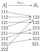 This example illustrates the following two properties of the map, : first, can be a proper subset of . As one can see from Theorem 1 below, is a proper subset of , if and only if . Second, two different words can have the same permutation type.
This example illustrates the following two properties of the map, : first, can be a proper subset of . As one can see from Theorem 1 below, is a proper subset of , if and only if . Second, two different words can have the same permutation type.We define another map, , by the following procedure:
- (i)
- Given a permutation, , we decompose the sequence, , of length L into maximal ascending subsequences. A subsequence, , of a sequence, , of length L is called a maximal ascending subsequence if it is ascending, namely, , and neither nor is ascending;
- (ii)
- If is a decomposition of into maximal ascending subsequences, then a word, , is defined by:We define . Note that , because π is the permutation type of some word, . Thus, we have . Hence, is well-defined as a map from to .
By construction, we have for all . To illustrate the construction of , let us consider a word, . The permutation type of is . The decomposition of into maximal ascending subsequences is 23, 145. We obtain by putting .
Theorem 1
- (i)
- For every ,where if . In particular, , if and only if ;
- (ii)
- Let us put:Then, restricted on is a map into and restricted on is a map into . They form a pair of mutually inverse maps. Furthermore, we have:
Proof.
The theorem is a recasting of statements in Lemma 5 and Theorem 9 in [17].
Let be a finite-alphabet stationary stochastic process, where each stochastic variable, , takes its value in . By the assumed stationarity, the probability of the occurrence of any word is time-shift invariant:
for all . Hence, it makes sense to define it without referring to the time to start. We denote the probability of the occurrence of a word, by . The probability of the occurrence of a permutation is given by .
For a finite-alphabet stationary stochastic process, , over the alphabet, , we define:
and:
where , , , and is the largest integer not greater than a.
Lemma 2
Let be a finite-alphabet stationary stochastic process and ϵ a positive real number. If for all , then we have .
Proof.
The claim follows from Theorem 1 (ii). See Lemma 12 in [17] for the complete proof.
3. A Result on Finite-State Finite-Alphabet Hidden Markov Models
In this paper, we use the parametric description of hidden Markov models as given in [27].
A finite-state finite-alphabet hidden Markov model (in short, HMM) [27] is a quadruple, , where Σ and A are finite sets, called state set and alphabet, respectively, is a family of matrices indexed by elements of A, where is the size of state set Σ, and μ is a probability distribution on the set Σ. The following conditions must be satisfied:
- (i)
- for any and ;
- (ii)
- for any ;
- (iii)
- and for any .
Two finite-alphabet stationary processes are induced by a HMM . One is solely determined by the underlying Markov chain. It is called an internal process and is denoted by . The alphabet for is Σ. The joint probability distributions that characterize is given by:
for any and . The other process with the alphabet, A, is defined by the following joint probability distributions:
for any and and is called an output process. The stationarity of the probability distribution μ ensures that of both the internal and output processes.
Symbols , such that occurs in the output process with a probability of zero. Hence, we obtain the equivalent output process, even if we remove these symbols. Thus, we can assume that for any without loss of generality.
The internal process, , of an HMM is called ergodic if the state transition matrix, T, is irreducible [28]: for any , there exists , such that . If the internal process, , is ergodic, then the stationary distribution μ is uniquely determined by the state transition matrix T via condition (iii). Every finite-alphabet finite-order multivariate stationary ergodic Markov process can be described as an HMM with an ergodic internal process.
Lemma 3
Let be the output process of an HMM , where is an ordered alphabet. If the internal process, , of the HMM is ergodic, then for every , there exists and , such that for all .
Proof.
Given , let us put . Fix an arbitrary . We have:
where and is the usual inner product of the -dimensional Euclidean space, . The spectral radius of the matrix is less than one. Indeed, this follows immediately from the Perron-Frobenius theorem for non-negative irreducible matrices: T is a non-negative irreducible matrix with by the assumption. Since and , applying Theorem 1.5 (e) in [29] implies that . By Lemma 5.6.10 in [30], for any , there exists a matrix norm, , such that . It follows that for any , there exists , such that for all :
where is the Euclidean norm. Since we have , we can choose , so that . If we put and , then we obtain by the Cauchy-Schwartz inequality as desired.
4. Permutation Complexity and Coupling Measures
In this section, we discuss the equalities between complexity and coupling measures and their permutation analogues for the output processes of HMMs whose internal processes are ergodic.
4.1. Fundamental Lemma
Let be a multivariate finite-alphabet stationary stochastic process, where each univariate process, , is defined over an ordered alphabet, . Note that the notation for stochastic variables is different from that in [17]. Here, is the stochastic variable for the k-th component of the multivariate process at time step t.
We use the notations:
and:
where , and for . In general, if , then and depend on and are invariant only by the simultaneous time shift . However, here, we make the dependence on implicit for notational simplicity.
Lemma 4
Let:
where:
and:
are the Shannon entropies of the joint occurrence of words and permutations , respectively, and the base of the logarithm is taken as two. Then, we have:
Proof.
We have:
By Theorem 1 (i), it holds that:
for such that .
If then:
On the other hand, we have:
This completes the proof of the inequality.
4.2. Excess Entropy
Let be a finite-alphabet stationary stochastic process. Its excess entropy is defined by [21]:
if the limit on the right-hand side exists, where is the entropy rate of , which exists for any finite-alphabet stationary stochastic process [31].
The excess entropy has been used as a measure of complexity [32,33,34,35,36,37]. Actually, it quantifies global correlations present in a given stationary process in the following sense. If exists, then it can be written as the mutual information between the past and future:
It is known that if is the output process of an HMM, then exists [38].
When the alphabet of is an ordered alphabet , we define the permutation excess entropy of by [17]:
if the limit on the right-hand side exists, where is the permutation entropy rate of , which exists for any finite-alphabet stationary stochastic process and is equal to the entropy rate [2,15,16, , and and are as defined in the statement of Lemma 4.
The following proposition is a generalization of our previous results in [17,18].
Proposition 5
Let be the output process of an HMM with an ergodic internal process. Then, we have:
where .
Proof.
Let . We have:
where , , and we have used for the first equality, Lemma 4 for the second inequality and Lemma 2 and Lemma 3 for the last inequality. By taking the limit, , we obtain .
To prove , it is sufficient to show that as . This is because we have:
However, this can be shown similarly with the above discussion by applying Lemma 4 to the bivariate process and, then, using Lemma 2 and Lemma 3.
4.3. Transfer Entropy and Momentary Information Transfer
In this subsection, we consider two information rates that are measures of coupling direction and strength between two jointly distributed processes and discuss the equalities between them and their permutation analogues. One is the rate of the transfer entropy [22], and the other is the rate of the momentary information transfer [24]. Both are particular instances of the conditional mutual information [39].
Let be a bivariate finite-alphabet stationary stochastic process. We assume that the alphabets of and are ordered alphabets, and , respectively. For , we define the τ-step transfer entropy rate from to by:
When , is called just the transfer entropy rate [40] from to and simply denoted by .
If we introduce the τ-step entropy rate of by:
and the τ-step conditional entropy rate of given by:
then we can write:
because both and exist. We call the conditional entropy rate and denote it by . Note that the conditional entropy rate here is slightly different from that found in the literature. For example, in [41], the conditional entropy rate (called the conditional uncertainty) is defined by . The difference from the conditional entropy rate defined here is in whether the conditioning on is involved or not.
is additive, namely, we always have:
However, for the τ-step conditional entropy rate, the additivity cannot hold in general. It is at most super-additive: we only have the inequality:
in general. Indeed, we have:
This leads to the sub-additivity of the τ-step transfer entropy rate:
An example with the strict inequality can be easily given. Let be an independent and identically distributed (i.i.d.) process and defined by and . We have and . Hence, for all .
There are two permutation analogues of the transfer entropy. One is called the symbolic transfer entropy (STE) [42], and the other is called the transfer entropy on rank vector (TERV) [43]. Here, we introduce their rates as follows: the rate of STE from to is defined by:
if the limit on the right-hand side exists. The rate of TERV from to is defined by:
if the limit on the right-hand side exists. If exists, then, by the definition of the permutation excess entropy, we have:
In this case, coincides with a quantity called the symbolic transfer entropy rate, introduced in [19].
Proposition 6
Let be the output process of an HMM with an ergodic internal process. Then, we have:
Proof.
Since both and are the output processes of appropriate HMMs with ergodic internal processes, the equalities follow from the similar discussion with that in the proof of Proposition 5. Indeed, for example, is the output process of the HMM , where .
A different instance of conditional mutual information, called momentary information transfer, is considered in [24]. It was proposed to improve the ability to detect coupling delays, which is lacking in the transfer entropy. Here, we consider its rate: the momentary information transfer rate is defined by:
Its permutation analogue, called the momentary sorting information transfer rate, is defined by:
By a similar discussion with that in the proof of Proposition 6, we obtain the following equality:
Proposition 7
Let be the output process of an HMM with an ergodic internal process. Then, we have:
4.4. Directed Information
Directed information is a measure of coupling direction and strength based on the idea of causal conditioning [26,44]. Since it is not a particular instance of conditional mutual information, here, we treat it separately. In the following presentation, we make use of terminologies from [40,45].
Let be a bivariate finite-alphabet stationary stochastic process. The alphabets of and are ordered alphabets, and , respectively. The directed information rate from to is defined by:
where:
Note that if in the above expression on the right-hand side is replaced by , then we obtain the mutual information between and :
Thus, conditioning on for , not on , distinguishes the directed information from the mutual information. Following [44], we write:
and call the quantity causal conditional entropy. By using this notation, we have:
The permutation analogue of the directed information rate, which we call the symbolic directed information rate is defined by:
if the limit on the right-hand side exists, where:
If we write:
and:
then we have the expressions:
Proposition 8
Let be the output process of an HMM with an ergodic internal process. Then, we have:
Proof.
We have:
We know that the first term on the right-hand side in the above inequality goes to zero as . Let us evaluate the second sum. By Lemma 4, it holds that:
By Lemma 2 and Lemma 3, we have:
where and . It is elementary to show that is finite. The limits of the other terms are also shown to be finite similarly. Thus, we can conclude that the limit of the second sum is bounded. Similarly, the limit of the third sum is also bounded. The equality in the claim follows immediately.
For output processes of HMMs with ergodic internal processes, properties on the directed information rate can be transferred to those on the symbolic directed information rate. Since proofs of them can be given by the same manner as those of the above propositions, here, we list some of them without proofs. For the proofs of the properties on the directed information rate, we refer to [44,45].
Let be the output process of an HMM with an ergodic internal process. Then, we have:
- (i)
- This is the permutation analogue of the equality:
- (ii)
- Here:and:The symbol, D, denotes the one-step delay. is the corresponding permutation analogue. The second equality is the permutation analogue of the equality . Since coincides with the transfer entropy rate, the first equality is just the equality between the transfer entropy rate and the symbolic transfer entropy rate (or the rate of one-step TERV) proven in Proposition 6, given the second equality;
- (iii)
- where is called the instantaneous information exchange rate and is defined by:and:From the last expression of , we can obtain:is the corresponding permutation analogue and called the symbolic instantaneous information exchange rate;
- (iv)
- Namely, the symbolic directed information rate decomposes into the sum of the symbolic transfer entropy rate and the symbolic instantaneous information exchange rate. This follows immediately from (ii), (iii) and the equality saying that the directed information rate decomposes into the sum of the transfer entropy rate and the instantaneous information exchange rate:
- (v)
- This is the permutation analogue of the equality saying that the mutual information rate between and is the sum of the directed information rate from to and the transfer entropy rate from to :where:is the mutual information rate and is its permutation analogue, called the symbolic mutual information rate. It is known that they are equal for any bivariate finite-alphabet stationary stochastic process [19]. Thus, the symbolic mutual information rate between and is the sum of the symbolic directed information rate from to and the symbolic transfer entropy rate from to .
We can also introduce the permutation analogue of the causal conditional directed information rate and prove the corresponding properties. To be precise, let us consider a multivariate finite-alphabet stationary stochastic process with the alphabet, . The causal conditional directed information rate from to given is defined by:
where:
Corresponding to Proposition 8, we have the following equality if is the output process of an HMM with an ergodic internal process:
where is the symbolic causal conditional directed information rate, which is defined in the same manner as the symbolic directed information rate. The following properties also hold: assume that is the output process of an HMM with an ergodic internal process. Then, we have:
- (i’)
- This is the permutation analogue of the equality:
- (ii’)
- The second equality is the permutation analogue of the equality:The quantities, and , are called the causal conditional transfer entropy rate and the symbolic causal conditional transfer entropyrate, respectively.
- (iii’)
- where is called the causal conditional instantaneous information exchange rate. The second equality is the permutation analogue of the equality:is the permutation analogue and is called the symbolic causal conditional instantaneous information exchange rate;
- (iv’)
- This is the permutation analogue of the following equality:
- (v’)
- This is the permutation analogue of the equality:where:is the causal conditional mutual information rate and is its permutation analogue, called the symbolic causal conditional mutual information rate. It can be shown that:if is the output process of an HMM with an ergodic internal process.
5. Discussion
In this section, we discuss how our theoretical results in this paper are related to the previous work in the literature.
Being confronted with real-world time series data, we cannot take the limit of a large length of words. Hence, we have to estimate information rates with a finite length of words. In such a situation, one permutation method could have some advantages over the other permutation methods. As a matter of fact, TERV was originally proposed as an improved analogue of STE [43]. However, it has been unclear whether they coincide in the limit of a large length of permutations. In this paper, we provide a partial answer to this question: the two permutation analogues of the transfer entropy rate, the rate of STE and the rate of TERV, are equivalent to the transfer entropy rate for bivariate processes generated by HMMs with ergodic internal processes.
The Granger causality graph [46] is a model of causal dependence structure in multivariate stationary stochastic processes. Given a multivariate stationary stochastic process, nodes in a Granger causality graph are components of the process. There are two types of edges: one is directed, and the other is undirected. The absence of a directed edge from one node to another node indicates the lack of the Granger cause from the former to the latter relative to the other remaining processes. Similarly, the absence of an undirected edge between two nodes indicates the lack of the instantaneous cause between them relative to the other remaining processes. Amblard and Michel [40,45] proposed that the Granger causality graph can be constructed based on directed information theory: let be a multivariate finite-alphabet stationary stochastic process with the alphabet, , and , the Granger causality graph of the process, , where is the set of nodes, is the set of directed edges and is the set of undirected edges. Their proposal is that:
- (i)
- for any , , if and only if ;
- (ii)
- for any , , if and only if .
Now, let us consider the case when is an output process of an HMM with an ergodic internal process. Then, from the results of Section 4.4, we have:
- (i’)
- for any , , if and only if ;
- (ii’)
- for any , , if and only if .
Real-world time series data are often multivariate. However, it seems that univariate analysis is still main stream in the field of ordinal pattern analysis (see, for example, the papers in [47]). We hope that this work stimulates multivariate analysis of real-world time series data.
Acknowledgments
The authors would like to thank D. Kugiumtzis for his useful comments and discussion on the relationship between STE and TERV. The authors also appreciate the anonymous referees for their comments, which significantly improved the manuscript. T.H. was supported by the Precursory Research for Embryonic Science and Technology (PRESTO) program of Japan Science and Technology Agency (JST).
Conflicts of Interest
The authors declare no conflict of interest.
References
- Bandt, C.; Pompe, B. Permutation entropy: A natural complexity measure for time series. Phys. Rev. Lett. 2002, 88, e174102. [Google Scholar] [CrossRef]
- Amigó, J.M. Permutation Complexity in Dynamical Systems; Springer-Verlag: Berlin/ Heidelberg, Germany, 2010. [Google Scholar]
- Bahraminasab, A.; Ghasemi, F.; Stefanovska, A.; McClintock, P.V.E.; Kantz, H. Direction of coupling from phases of interacting oscillators: A permutation information approach. Phys. Rev. Lett. 2008, 100, e084101. [Google Scholar] [CrossRef]
- Cao, Y.H.; Tung, W.W.; Gao, J.B.; Protopopescu, V.A.; Hively, L.M. Detecting dynamical changes in time series using the permutation entropy. Phys. Rev. E 2004, 70, e046217. [Google Scholar] [CrossRef]
- Kugiumtzis, D. Partial transfer entropy on rank vectors. Eur. Phys. J. Special Topics 2013, 222, 401–420. [Google Scholar] [CrossRef]
- Nakajima, K.; Haruna, T. Symbolic local information transfer. Eur. Phys. J. Special Topics 2013, 222, 421–439. [Google Scholar] [CrossRef]
- Rosso, O.A.; Larrondo, H.A.; Martin, M.T.; Plastino, A.; Fuentes, M.A. Distinguishing noise from chaos. Phys. Rev. Lett. 2007, 99, e154102. [Google Scholar] [CrossRef]
- Amigó, J.M.; Keller, K. Permutation entropy: One concept, two approaches. Eur. Phys. J. Special Topics 2013, 222, 263–273. [Google Scholar] [CrossRef]
- Bandt, C.; Keller, G.; Pompe, B. Entropy of interval maps via permutations. Nonlinearity 2002, 15, 1595–1602. [Google Scholar] [CrossRef]
- Keller, K.; Sinn, M. A standardized approach to the Kolmogorov-Sinai entropy. Nonlinearity 2009, 22, 2417–2422. [Google Scholar] [CrossRef]
- Keller, K.; Sinn, M. Kolmogorov-Sinai entropy from the ordinal viewpoint. Phys. D 2010, 239, 997–1000. [Google Scholar] [CrossRef]
- Keller, K. Permutations and the Kolmogorov-Sinai entropy. Discr. Cont. Dyn. Syst. 2012, 32, 891–900. [Google Scholar] [CrossRef]
- Keller, K.; Unakafov, A.M.; Unakafova, V.A. On the relation of KS entropy and permutation entropy. Phys. D 2012, 241, 1477–1481. [Google Scholar] [CrossRef]
- Unakafova, V.A.; Unakafov, A.M.; Keller, K. An approach to comparing Kolmogorov-Sinai and permutation entropy. Eur. Phys. J. Special Topics 2013, 222, 353–361. [Google Scholar] [CrossRef]
- Amigó, J.M.; Kennel, M.B.; Kocarev, L. The permutation entropy rate equals the metric entropy rate for ergodic information sources and ergodic dynamical systems. Phys. D 2005, 210, 77–95. [Google Scholar] [CrossRef]
- Amigó, J.M. The equality of Kolmogorov-Sinai entropy and metric permutation entropy generalized. Phys. D 2012, 241, 789–793. [Google Scholar] [CrossRef]
- Haruna, T.; Nakajima, K. Permutation complexity via duality between values and orderings. Phys. D 2011, 240, 1370–1377. [Google Scholar] [CrossRef]
- Haruna, T.; Nakajima, K. Permutation excess entropy and mutual information between the past and future. Int. J. Comput. Ant. Sys. 2012, in press. [Google Scholar]
- Haruna, T.; Nakajima, K. Symbolic transfer entropy rate is equal to transfer entropy rate for bivariate finite-alphabet stationary ergodic Markov processes. Eur. Phys. J. B 2013, 86, e230. [Google Scholar] [CrossRef]
- Haruna, T.; Nakajima, K. Permutation approach to finite-alphabet stationary stochastic processes based on the duality between values and orderings. Eur. Phys. J. Special Topics 2013, 222, 383–399. [Google Scholar] [CrossRef]
- Crutchfield, J.P.; Feldman, D.P. Regularities unseen, randomness observed: Levels of entropy convergence. Chaos 2003, 15, 25–54. [Google Scholar] [CrossRef]
- Schreiber, T. Measuring information transfer. Phys. Rev. Lett. 2000, 85, 461–464. [Google Scholar] [CrossRef] [PubMed]
- Kaiser, A.; Schreiber, T. Information transfer in continuous processes. Phys. D 2002, 166, 43–62. [Google Scholar] [CrossRef]
- Pompe, B.; Runge, J. Momentary information transfer as a coupling measure of time series. Phys. Rev. E 2011, 83, e051122. [Google Scholar] [CrossRef]
- Marko, H. The bidirectional communication theory—A generalization of information theory. IEEE Trans. Commun. 1973, 21, 1345–1351. [Google Scholar] [CrossRef]
- Massey, J.L. Causality, Feedback and Directed Information. In Proceedings of International Symposium on Information Theory and Its Applications, Waikiki, HI, USA, 27–30 November 1990.
- Anderson, B.D.O. The realization problem for hidden Markov models. Math. Control Signals Syst. 1999, 12, 80–120. [Google Scholar] [CrossRef]
- Walters, P. An Introduction to Ergodic Theory; Springer-Verlag: New York, NY, USA, 1982. [Google Scholar]
- Seneta, E. Non-Negative Matrices and Markov Chains; Springer: New York, NY, USA, 1981. [Google Scholar]
- Horn, R.A.; Johnson, C.R. Matrix Analysis; Cambridge University Press: Cambridge, UK, 1985. [Google Scholar]
- Cover, T.M.; Thomas, J.A. Elements of Information Theory, 2nd ed.; John Wiley & Sons, Inc.: Hoboken, NJ, USA, 2006. [Google Scholar]
- Arnold, D.V. Information-theoretic analysis of phase transitions. Complex Syst. 1996, 10, 143–155. [Google Scholar]
- Bialek, W.; Nemenman, I.; Tishby, N. Predictability, complexity, and learning. Neural Comput. 2001, 13, 2409–2463. [Google Scholar] [CrossRef] [PubMed]
- Feldman, D.P.; McTague, C.S.; Crutchfield, J.P. The organization of intrinsic computation: Complexity-entropy diagrams and the diversity of natural information processing. Chaos 2008, 18, e043106. [Google Scholar] [CrossRef] [PubMed]
- Grassberger, P. Toward a quantitative theory of self-generated complexity. Int. J. Theor. Phys. 1986, 25, 907–938. [Google Scholar] [CrossRef]
- Li, W. On the relationship between complexity and entropy for Markov chains and regular languages. Complex Syst. 1991, 5, 381–399. [Google Scholar]
- Shaw, R. The Dripping Faucet as a Model Chaotic System; Aerial Press: Santa Cruz, CA, USA, 1984. [Google Scholar]
- Löhr, W. Models of Discrete Time Stochastic Processes and Associated Complexity Measures. Ph.D. Thesis, Max Planck Institute for Mathematics in the Sciences, Leipzig, Germany, 2010. [Google Scholar]
- Frenzel, S.; Pompe, B. Partial mutual information for coupling analysis of multivariate time series. Phys. Rev. Lett. 2007, 99, e204101. [Google Scholar] [CrossRef]
- Amblard, P.O.; Michel, O.J.J. On directed information theory and Granger causality graphs. J. Comput. Neurosci. 2011, 30, 7–16. [Google Scholar] [CrossRef] [PubMed]
- Ash, R. Information Theory; Wiley Interscience: New York, NY, USA, 1965. [Google Scholar]
- Staniek, M.; Lehnertz, K. Symbolic transfer entropy. Phys. Rev. Lett. 2008, 100, e158101. [Google Scholar] [CrossRef]
- Kugiumtzis, D. Transfer entropy on rank vectors. J. Nonlin. Sys. Appl. 2012, 3, 73–81. [Google Scholar]
- Kramer, G. Directed Information for Channels with Feedback. Ph.D. Thesis, Swiss Federal Institute of Technology, Zurich, Switzerland, 1998. [Google Scholar]
- Amblard, P.O.; Michel, O.J.J. Relating Granger causality to directed information theory for networks of stochastic processes. 2011; arXiv:0911.2873v4. [Google Scholar]
- Dahlaus, R.; Eichler, M. Causality and graphical models in time series analysis. In Highly Structured Stochastic Systems; Green, P., Hjort, N., Richardson, S., Eds.; Oxford University Press: New York, NY, USA, 2003; pp. 115–137. [Google Scholar]
- European Physical Journal Special Topics on Recent Progress in Symbolic Dynamics and Permutation Complexity. Eur. Phys. J. 2013, 222, 241–598.
© 2013 by the authors; licensee MDPI, Basel, Switzerland. This article is an open access article distributed under the terms and conditions of the Creative Commons Attribution license (http://creativecommons.org/licenses/by/3.0/).