Article

Kernel Spectral Clustering for Big Data Networks

Department of Electrical Engineering ESAT/SCD (SISTA), Katholieke Universiteit Leuven, Kasteelpark Arenberg 10, B-3001 Leuven, Belgium
*
Author to whom correspondence should be addressed.
Entropy 2013, 15(5), 1567-1586; https://doi.org/10.3390/e15051567
Submission received: 1 March 2013 / Revised: 25 April 2013 / Accepted: 29 April 2013 / Published: 3 May 2013
(This article belongs to the Special Issue Big Data)

Abstract

:
This paper shows the feasibility of utilizing the Kernel Spectral Clustering (KSC) method for the purpose of community detection in big data networks. KSC employs a primal-dual framework to construct a model. It results in a powerful property of effectively inferring the community affiliation for out-of-sample extensions. The original large kernel matrix cannot fitinto memory. Therefore, we select a smaller subgraph that preserves the overall community structure to construct the model. It makes use of the out-of-sample extension property for community membership of the unseen nodes. We provide a novel memory- and computationally efficient model selection procedure based on angular similarity in the eigenspace. We demonstrate the effectiveness of KSC on large scale synthetic networks and real world networks like the YouTube network, a road network of California and the Livejournal network. These networks contain millions of nodes and several million edges.

1. Introduction

In the modern era, complex networks are ubiquitous. Their omnipresence is reflected in domains like social networks, web graphs, road graphs, communication networks, biological networks and financial networks. Complex networks can be represented as graphs ( G ( V , E ) ), where the nodes (V) represent vertices in the graph and edges (E) depict the relationship between these nodes. These networks exhibit community like structure, where nodes within a community are densely connected and the connections are sparse between the communities. The problem of community detection has also been framed as graph partitioning and graph clustering [1] and has received a lot of attention lately [2,3,4,5,6,7,8,9,10,11,12,13]. Among the myriad variety of algorithms for community detection, the Kernel Spectral Clustering (KSC) method is related to the spectral clustering methods [10,11,12,13]. Spectral clustering methods are standard techniques for graph partitioning. The underlying model is based on eigen-decomposition of the Laplacian matrix derived from the affinity matrix of the nodes in the community. The major drawback of these spectral clustering methods is the construction of the large affinity matrix ( N × N ), where N is the number of nodes in the network, which requires to calculate the similarity between every pair of nodes in the network. As the size of the network increases, the O ( N 2 ) computation and storage of this affinity N × N matrix become infeasible.
Recently, a spectral clustering formulation based on weighted kernel PCA with primal-dual framework was proposed in [14]. The formulation resulted in a model with a powerful property of inferring community memberships for out-of-sample nodes. The model is built on a small subset of the big data network that captures the inherent community structure. One then solves an affordable eigenvalue problem on this smaller subgraph and uses the out-of-sample extension property. The KSC method was extended for community detection by [8]. However, the two important steps, the subset selection and the model selection proposed by [8], are computationally expensive and memory inefficient. The two major contributions of the paper are:
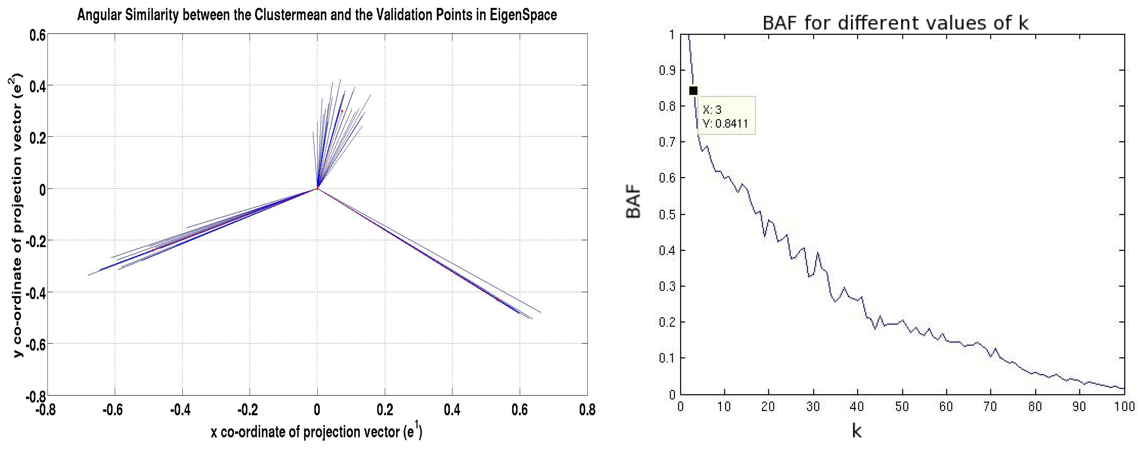
  • We propose a novel memory-and computationally efficient model selection technique to tune the parameter of the model using angular similarity in the eigenspace between the projected vectors of the nodes in the validation set.
  • We show that kernel spectral clustering is applicable for community detection in big data networks.
The authors in [8] utilized Modularity [15] for the purpose of model selection. However, they need to keep a square, non-sparse N × N matrix for validation of the model using Modularity. This makes the approach infeasible when the networks are large scale. We provide a novel model selection technique based on angular similarity between the projected vectors in the eigen-spectrum. The authors in [8] used Expansion sampling [16] technique for subset selection. The method is based on the principle of expander graphs and optimizes the expansion factor function. However, the method is computationally expensive as shown in [17] and stochastic by nature. Therefore, for the given big data network, for each iteration of Expansion sampling, the obtained subgraph would be different. We use the Fast and Unique Representative Subset (FURS) selection technique [17] for obtaining a representative subset of the big data network. The method is computationally less expensive and is a better representative of the community structure than most of the state-of-the-art sampling techniques like SlashBurn [18], Metropolis [19], Snowball Expansion [16], Random Node [20] sampling, etc., as shown through extensive comparisons in [17]. The KSC method was recently extended to evolving networks as described in [21]. In this paper, all considered graphs are unweighted and undirected unless specified otherwise. All the experiments were performed on a machine with 12 GB RAM and 2.4 GHz Intel Xeon processor. The maximum size of the kernel matrix that can be stored in the memory of our PC is 5 , 000 × 5 , 000 . The approach that we present can be easily implemented in a distributed environment as well and can handle big data networks.
The rest of the paper is organized as the follows. Section 2 provides details about the kernel spectral clustering method. Section 3 describes the angular similarity based model selection procedure. Section 4 gives insight into the FURS selection technique to obtain a representative subgraph. Section 5 describes the experiments undertaken along with the results on big data networks. We conclude in Section 6.

2. Kernel Spectral Clustering

We first provide details about the notations used.

2.1. Notations

(1)
A graph is mathematically represented as G = ( V , E ) where V represents the set of nodes and E V × V represents the set of edges in the network. Physically, the nodes represent the entities in the network and the edges represent the relationship between these entities.
(2)
The cardinality of the set V is denoted as N.
(3)
The cardinality of the set E is denoted as e.
(4)
The matrix A is a N × N matrix and represents the affinity or similarity matrix.
(5)
For unweighted graphs, A is called the adjacency matrix and A i j = 1 if ( v i , v j ) E , otherwise A i j = 0 .
(6)
The subgraph generated by the subset of nodes S is represented as G ( S ) . Mathematically, G ¯ = ( S , Q ) where S V and Q = ( S × S ) E represents the set of edges in the subgraph.
(7)
The degree distribution function is given by f ( V ) . For the graph G it can written as f ( V ) while for the subgraph S it can be presented as f ( S ) . Each vertex v i V has a degree represented as f ( v i ) .
(8)
The degree matrix is represented as D, a diagonal matrix with diagonal entries d i , i = j A i j .
(9)
The adjacency list corresponding to each vertex v i V is given by A ( i , : ) .
(10)
The neighboring nodes of a given node v i are represented by N b r ( v i ) .
(11)
The median degree of the graph is represented as M.

2.2. General Background

Spectral clustering uses the information contained in the affinity matrix to detect structures in the given network. In case of data points, the similarity between the points is measured with respect to the mutual distance (e.g., Euclidean, cosine, RBF distance) between the points. Thus, the obtained similarity matrix can be considered as a weighted graph where each point has a certain extent of similarity with other points in the dataset. For our case, we already have a weighted graph A, where A i j = 1 if ( v i , v j ) E else A i j = 0 . Therefore, in our case the spectral clustering method can be applied directly. However, for the KSC method, we need to build a graph over the network to represent the similarity between the nodes in a kernel based framework.
The spectral graph theory can provide insights into several properties of the graph-like partitions existing in the graph. These insights are obtained by studying the eigen-spectrum of the Laplacian matrix [10,11,22]. Several Laplacian matrices exist, including the unnormalized Laplacian defined as L = D - A , the symmetric normalized Laplacian L S Y M = D - 1 / 2 L D - 1 / 2 = I N - D - 1 / 2 A D - 1 / 2 , the non-symmetric normalized Laplacian L R W = D - 1 L = I N - D - 1 A . This Laplacian is related to the random walk on the graph, hence denoted by L R W . For a random walk Laplacian, clustering can be understood as detecting the partitions such that a random walker will spend maximum time in that partition with a few jumps to other clusters. This minimizes the transition probability between the clusters. The transition matrix of the random walker on the graph can be obtained by normalizing the adjacency matrix A such that the sum of its row ends up being 1. Thus the transition matrix can be depicted as P = D - 1 A , where the entry P i j represents the probability of a jump from node v i to node v j . The corresponding eigenvalue problem becomes P r = ξ r and was shown to be the dual problem of a constrained optimization problem typical of least squares support vector machines (LS-SVM) [23].

2.3. Primal-Dual Formulation

The KSC method is described by a primal-dual framework. The model is determined during the training phase, and the parameter of the model, i.e., k (number of clusters), is estimated during the validation stage. Finally, the model is tested on the test data to provide community affiliation to the unseen nodes.
In case of networks, the training data comprises the adjacency list of all the vertices v i X t r , where X t r represents the set of nodes used for training the model. Let the cardinality of the set X t r be N t r . Big data networks can be stored into memory in sparse format as these networks are highly sparse. However, if the graph does not fit in the main memory, it can be split into blocks of adjacency lists and stored on the hard disk. We can then iterate over these blocks by selecting the adjacency lists corresponding to the nodes in the training set X t r . This set of adjacency lists can be efficiently stored in the memory as real world networks are highly sparse and there are very few connections for each node v i X t r . The maximum length of the adjacency list of a node in the training data can be equal to N, when the node is connected to all the other nodes in the network. During the test phase, the cluster memberships for each of the unseen nodes can be predicted by uploading the adjacency list of the test node in the memory and using the out-of-sample extension property of the model. This makes the approach feasible for big data networks, unlike approaches that require the entire graph to be stored in the main memory. Moreover, the computational complexity of our approach is dominated by the time required to construct the kernel matrix. It is given by O ( N t r 2 N ) , i.e., the time required to calculate the similarity between sparse adjacency lists of the nodes in the training data.
Given X t r training nodes D = { x i } i = 1 N t r , x i R N and x i X t r . Here x i represents the adjacency list of the i t h training node and the number of nodes in the training set is N t r . Given D and the number of communities k, the primal problem of the spectral clustering via weighted kernel PCA is formulated as follows [14]:
min w ( l ) , e ( l ) , b l 1 2 l = 1 k - 1 w ( l ) w ( l ) - 1 2 N l = 1 k - 1 γ l e ( l ) D Ω - 1 e ( l ) such that e ( l ) = Φ w ( l ) + b l 1 N t r , l = 1 , , k - 1
where e ( l ) = [ e 1 ( l ) , , e N t r ( l ) ] are the projections onto the eigenspace, l = 1 , , k - 1 indicates the number of score variables required to encode the k communities, D Ω - 1 R N t r × N t r is the inverse of the degree matrix associated to the kernel matrix Ω. Φ is the N t r × d h feature matrix, Φ = [ ϕ ( x 1 ) ; ; ϕ ( x N t r ) ] and γ l R + are the regularization constants. We note that N t r N , i.e., the number of nodes in the training set, is much less than the total number of nodes in the big data network. The kernel matrix Ω is the obtained by calculating the similarity between the adjacency list of each pair of nodes in the training set. Each element of Ω, denoted as Ω i j = K ( x i , x j ) = ϕ ( x i ) ϕ ( x j ) , is obtained by calculating the cosine similarity between the adjacency lists of x i and x j , which has been shown to be an effective similarity measure for large scale data [24]. Thus, Ω i j = x i x j x i x j and can be calculated efficiently using notions of set unions and intersections. This corresponds to using a normalized linear kernel function K ( x , z ) = x z x z [23]. The clustering model is then represented by:
e i ( l ) = w ( l ) ϕ ( x i ) + b l , i = 1 , , N t r
where ϕ : R N R d h is the mapping to a high-dimensional feature space d h , b l are the bias terms, l = 1 , , k - 1 . However, for big data networks we can utilize the explicit expression of the underlying feature map and d h = R N . The projections e i ( l ) represent the latent variables of a set of k - 1 binary cluster indicators given by sign ( e i ( l ) ) , which can be combined with the final groups using an encoding/decoding scheme. The dual problem corresponding to this primal formulation is:
D Ω - 1 M D Ω α ( l ) = λ l α ( l )
where M D is the centering matrix, which is defined as M D = I N t r - ( 1 1 N t r D Ω - 1 1 N t r ) ( 1 N t r 1 N t r D Ω - 1 ) . The α ( l ) are the dual variables and the kernel function K : R N × R N R plays the role of similarity function. This dual problem is closely related to the random walk model.

2.4. Encoding/Decoding Scheme

In ideal situations when the communities are non-overlapping, we will obtain k well separated clusters and the matrix D - 1 M D Ω has k - 1 piece-wise constant eigenvectors. This is because the multiplicity of the largest eigenvalue (i.e., 1) is k - 1 as depicted in [22]. In the eigenspace every cluster A p , p = 1 , , k is a point and is represented with a unique codebook c p { - 1 , 1 } k - 1 . To obtain this codebook CB = { c p } p = 1 k we transform the rows of the projected vector matrix obtained from the training data by binarizing it, i.e., [ sign ( e ( 1 ) , , e ( k - 1 ) ) ] . However, in real world networks, the communities do overlap and we have nearly piece-wise constant eigenvectors. The codebook set CB is also obtained by selecting the top k most frequent codebook vectors. Due to the centering matrix M D , the eigenvectors have zero mean and the optimal threshold for binarizing the eigenvectors is self-determined (equal to 0). Taking into account that the first eigenvector α ( 1 ) already provides a binary clustering, the number of score variables needed to encode k clusters is k - 1 . The decoding scheme consists of comparing the cluster indicators obtained in the validation/test stage with the codebook and selecting the nearest codebook based on Hamming distance. This scheme corresponds to the ECOC decoding procedure [25] and is used in out-of-sample extensions as well. The proposed extension is based on the score variables, which correspond to the projections of the mapped out-of-sample points onto the eigenvectors found in the training stage. The cluster indicators can be obtained by binarizing the score variables for the out-of-sample points as follows:
sign ( e t e s t ( l ) ) = sign ( Ω t e s t α ( l ) + b l 1 N t e s t )
where l = 1 , , k - 1 , Ω t e s t is the N t e s t × N t r kernel matrix evaluated using the test points with entries Ω t e s t , r i = K ( x r t e s t , x i ) , r = 1 , , N t e s t and i = 1 , , N t r . Here N t e s t represents the number of nodes in the test set. This natural extension to out-of-sample points is the main advantage of the kernel spectral clustering framework. In this way the clustering model can be trained, validated and tested in an unsupervised learning procedure. If the Ω t e s t cannot fit the memory, then we divide the test set into blocks and perform the testing operations iteratively on a single computer. However, this operation can easily be performed in parallel in a distributed environment.

3. Model Selection by Means of Angular Similarity

Model selection is a crucial step in KSC. In order to obtain correct cluster parameters for the model, we propose a novel and computationally efficient mechanism using the concept of angular similarity. In [8], the authors used Modularity as a model selection criterion. However, the validation matrix required for Modularity calculation can blow up as the size of the network becomes large and might be infeasible to store into memory. Therefore, we need to work with the sparse adjacency lists of the nodes in the validation set instead of creating a square validation matrix. Since we are using the cosine similarity metric to estimate each element of the kernel matrix Ω, the model is free of a tuning parameter σ, unlike the original formulation of KSC [14] when using a Gaussian RBF kernel. Thus, the only parameter to be determined for our procedure is the number of clusters k in the network.
We propose a criterion Balanced Angular Fit for estimating the number of clusters k > 2 in the network. This criterion exploits the projections of the training and validation nodes in the eigenspace. For a given value of k > 2 , we estimate the cluster memberships of the nodes in the training set X t r based on the codebook CB . We assign each training node to the cluster corresponding to the codebook vector for which its Hamming distance is the minimum. Thus, for a given value of k > 2 , we can obtain the clustering Δ = { P 1 , , P k } , where P i contains the set of training nodes belonging to the i t h cluster. We calculate the cluster mean ( μ i ) for each cluster w.r.t. to the projections of the training nodes belonging to the i t h cluster in the eigenspace.
Once we obtain the cluster means for all the clusters, we use the projections of the validation nodes in the eigenspace. The idea is to calculate the angular similarity between the projection of each validation node and each of the cluster means. The cluster mean that makes the least angle with the projection of the validation node is the closest or most similar for that node. Thus, we assign the cluster corresponding to that cluster mean to the given validation node. For each validation node ( v a l i d i ), we want to obtain max j cos ( θ j , v a l i d i ) , where
c o s ( θ j , v a l i d i ) = μ j e v a l i d i μ j e v a l i d i , j = 1 , , k .
The closer the projection of the validation node is to that of a given cluster mean, the smaller the angle it has with it and the larger the cosine value of that angle. Therefore, for each validation node we have the cluster to which it is assigned along with the maximum cosine similarity value. We maintain the maximum cosine similarity value for each validation node in a dictionary M a x S i m . The dictionary is maintained as M a x S i m ( v a l i d i ) = cos ( θ j , v a l i d i ) , where cos ( θ j , v a l i d i ) = max j cos ( θ j , v a l i d i ) , j = 1 , , k is the maximum cosine similarity value for the validation node ( v a l i d i ). The obtained clustering is Δ v a l i d = { Q 1 , , Q k } , where Q i contains the set of validation nodes belonging to cluster i. We now define Balanced Angular Fit ( B A F ) as:
B A F ( k ) = i = 1 k v a l i d j Q i 1 k . M a x S i m ( v a l i d j ) | Q i |
The B A F simply sums up the cosine similarity values of all the validation nodes belonging to each cluster divided by the cardinality of that cluster. It then divides this overall value by the total number of clusters k in the network. The range of values that B A F can take is [ - 1 , 1 ] . This is because the maximum similarity value that a validation node can have w.r.t. a cluster mean is 1 (i.e., the angle between them is zero). Because we sum up the cosine similarity values of all the validation nodes in a cluster and divide it by the cardinality of that cluster, the metric is inherently balanced and this fraction cannot exceed one. This process is repeated for each cluster, and in order to normalize the metric, we divide it by the number of clusters in the network. In the worst case scenario, when all the validation nodes are wrongly assigned to clusters with whose cluster mean it makes an angle of π, the B A F can end up being - 1 . However, we observed empirically that the B A F value ranges between [ 0 , 1 ] in all our experiments. Higher values of B A F indicate better graph partitions found in the validation set. To estimate the parameter k, we iteratively increase the value of k from 3 till a maximum value and select the value of k for which the B A F is maximum. The B A F will not work for k = 2 as the cluster mean obtained are one-dimensional, one value is positive and the other is negative. The projections of validation nodes are also one-dimensional and either positive or negative and thus the minimum angle between the projections of the validation nodes and the best cluster mean will always be zero. Thus, the B A F value will turn out to be 1. The B A F measure can not only be used as a model selection criterion but also serve the purpose of an evaluation metric for testing the quality of the clustering. There can be several values of k for which the B A F values can be high. If the interval between these values of k is large, then it can be identified with the underlying hierarchy in the network.
In Figure 1, the red colored “*” marked points represent the cluster means in 2-D projected eigenspace where the number of cluster k in the network is equal to 3. The projections of the validation nodes are represented as blue colored “.” points in 2-D. From Figure 1, one can easily conclude the presence of three clusters and the same can be inferred by B A F . We can observe that angle between the projections of the validation points and the corresponding best cluster mean is quite small. This is also inferred from the high B A F value of 0 . 8411 for k = 3 . We also observe that the nodes in the validation set whose projections are in the first quadrant have maximum deviation from their cluster mean, which affects the overall B A F value. From the figure on the right, we observe that for k = 2 , the B A F value is equal to 1 as suggested earlier and thus ignored while reporting the correct number of clusters.
Figure 1. Model Selection for KSC based on B A F .
Entropy 15 01567 g001

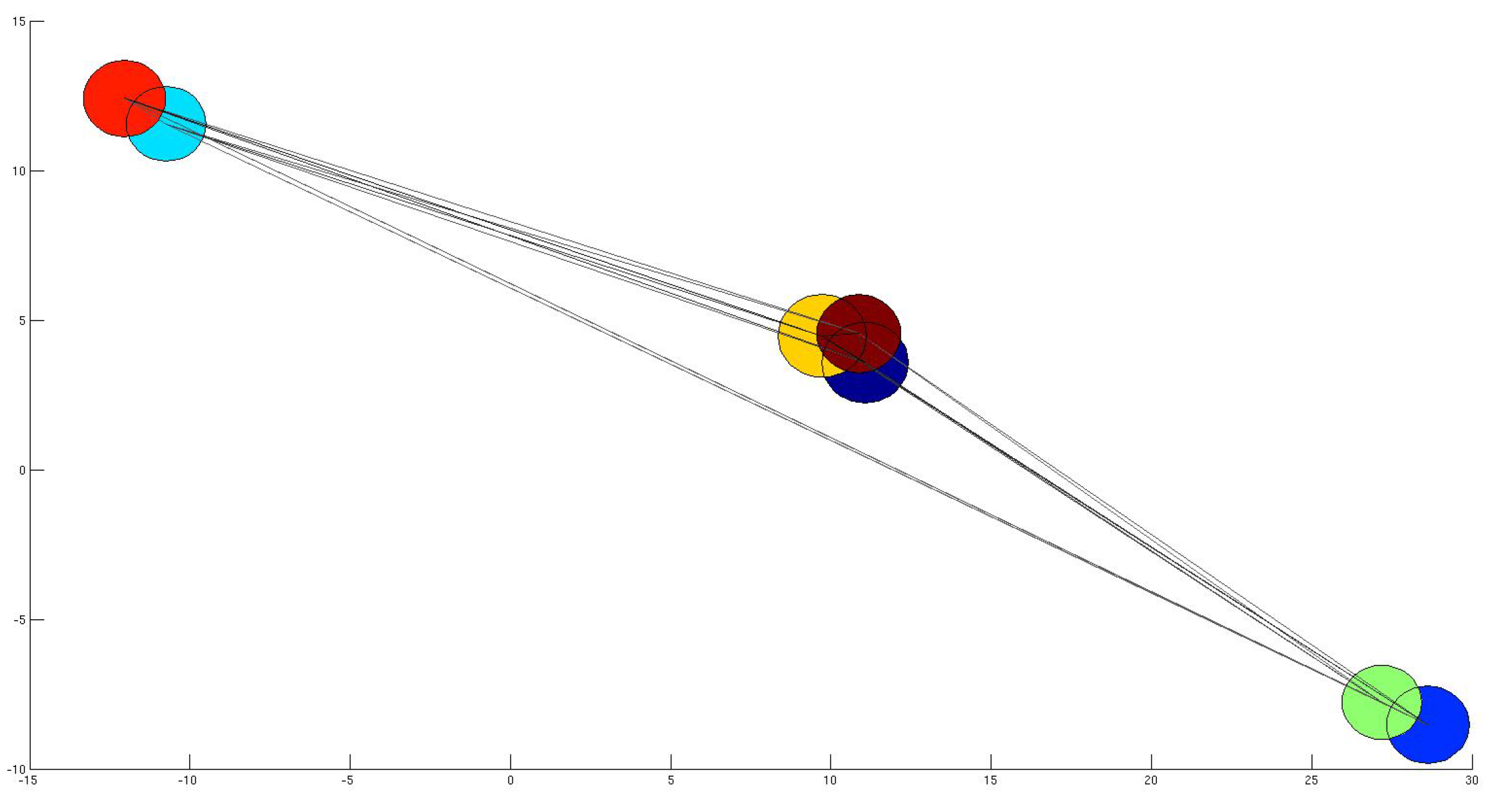
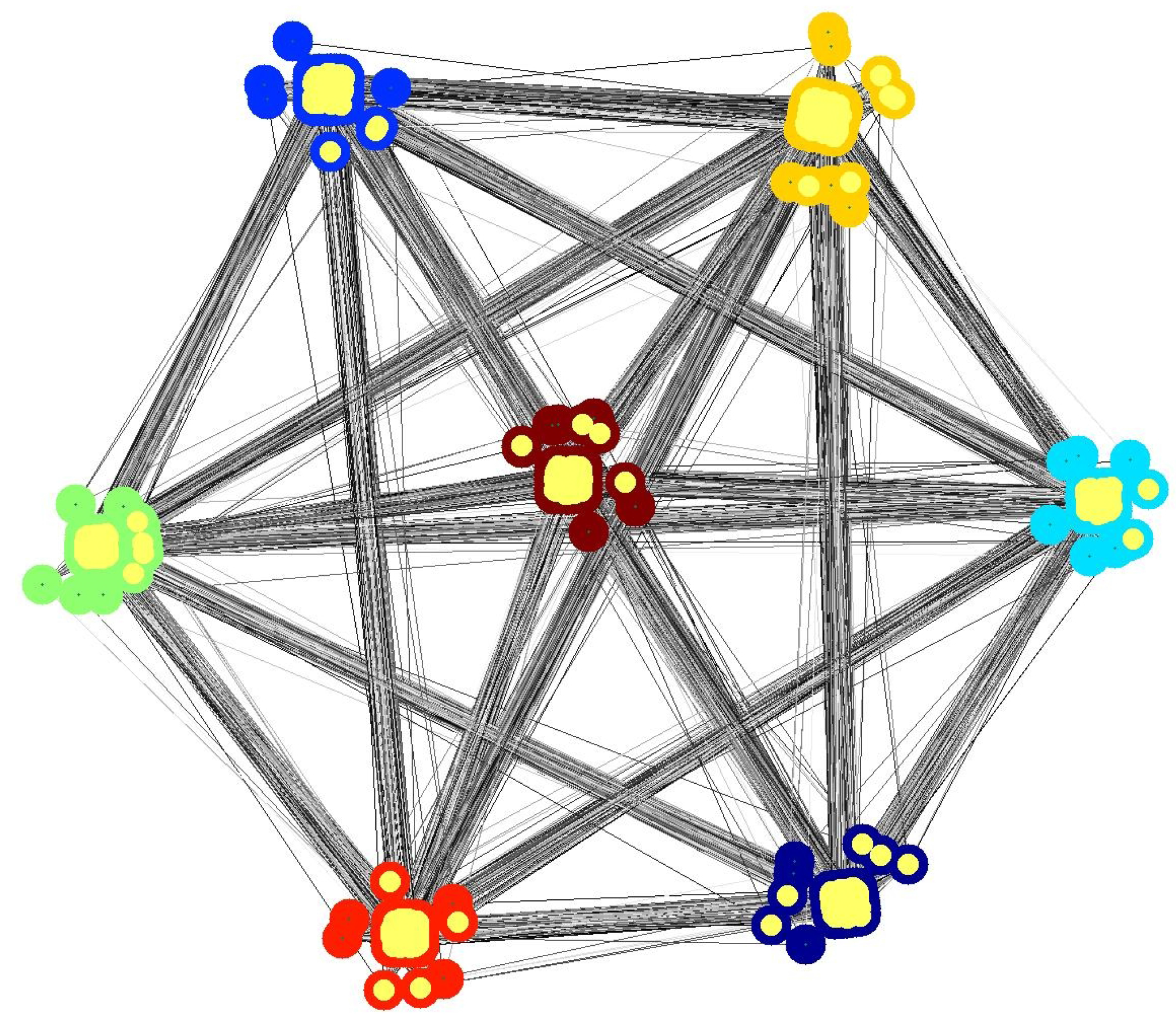
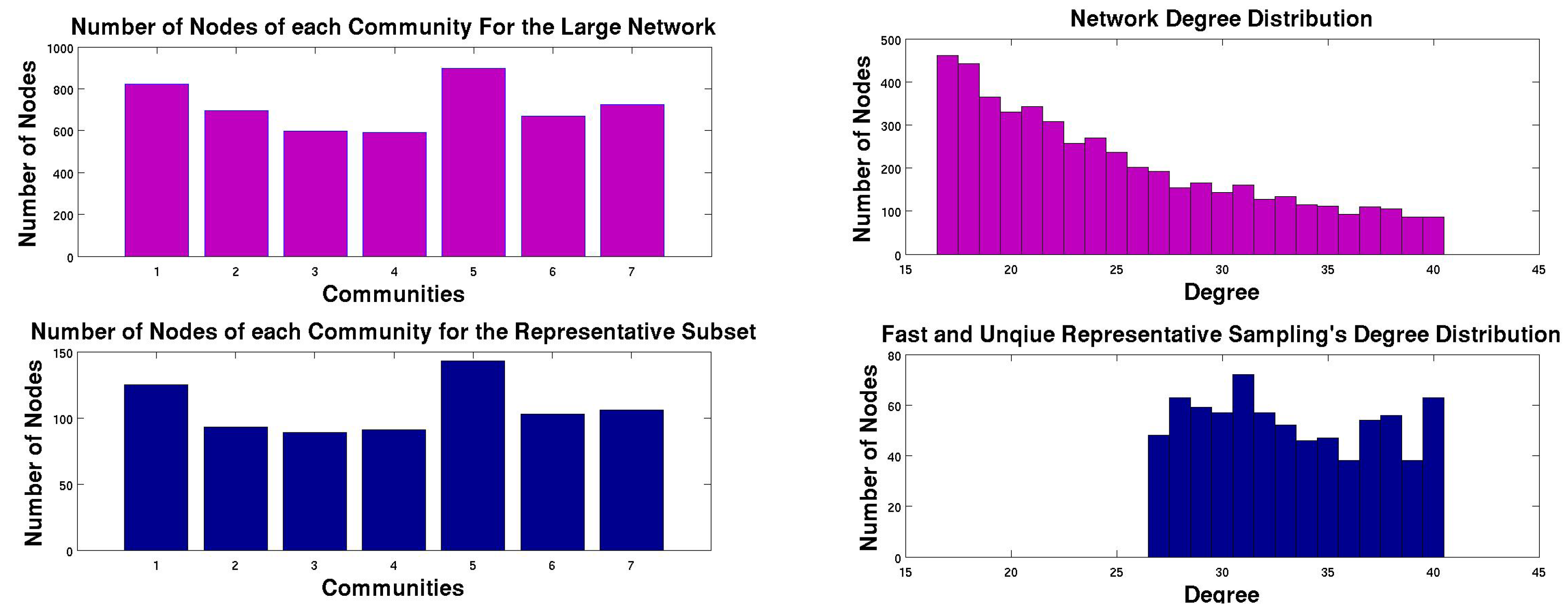
4. Selecting a Representative Subgraph

An inherent requirement of the KSC method is to generate a model on the training set. Since, KSC generates a N t r × N t r size kernel matrix, if the size of N t r becomes too large then the KSC procedure would become infeasible. Thus, we need to select a subset of nodes that is representative for the underlying community structure. The obtained subgraph allows to build a model on it during the training phase and provides a meaningful out-of-sample extension to nodes that are not present in the training set. State-of-the-art techniques for sampling large scale graphs include SlashBurn algorithm [18], Snowball Expansion sampling [16], Metropolis [19] and random sampling techniques. An exhaustive comparison of these methods with Fast and Unique Representative Subset (FURS) selection approach was done in [17]. FURS is computationally less expensive and preserves the inherent community structure as evaluated on the various quality metrics like computation time, clustering coefficient, degree distribution, coverage, fraction of communities preserved and variation of information metric, as described in [17].
The motivation is to select a subset of nodes that approximately maximizes the coverage of the graph under the constraint that the selected nodes belong to different dense regions in the graph. Coverage is defined as the ratio of the number of unique nodes directly reachable from the nodes in the selected subset to the total number of nodes in the graph. Coverage is determined by the degree distribution of the nodes in the graph. The idea is to first sort the nodes based on their degree in descending order during each iteration and pick the node with highest degree. Once such a node is selected, its immediate neighbors are deactivated (as they can be reached directly from this node) during that iteration and the node is placed in the selected subset without affecting the graph topology. We then select the node with highest degree among the active nodes and the process is repeated until either all the nodes are deactivated or we reach the subset size. If all nodes are deactivated before we reach the desired subset size, a new iteration is started and the deactivated nodes are reactivated. They are sorted according to their degree in descending order and the process of node selection, deactivation and reactivation is repeated till we obtain the desired subset. FURS results in a subset of nodes that span most or all of the communities in the network. We outline the FURS approach in Algorithm 1.
Entropy 15 01567 i001
For big data networks, which cannot fit into memory, FURS can be applied to each individual block of the network that can be stored into memory. Thus, the obtained subset would approximately maximize the coverage of the network and capture the inherent community structure.

4.1. Subset Selection from Synthetic Network

We first demonstrate the FURS selection technique on a small synthetic network. The synthetic graph was generated by the software provided by Fortunato as mentioned in [6]. This software is used to generate an undirected and unweighted synthetic graph of 5 , 000 nodes with 125 , 020 edges and 7 communities. The software allows to set a mixing parameter μ that reflects the extent of overlap among the communities. We set the mixing parameter to a moderate value of μ = 0 . 1 (higher values of mixing parameter lead to highly overlapped communities). Figure 2 depicts the communities as discs of different colors and reflects the extent of overlap between these communities.
In Figure 2, we do not highlight all the nodes and all the edges. Rather, we show the communities as discs. The communities that are overlapping have more connections among themselves as in comparison with their connections to the other communities.
Figure 2. Communities and their extent of overlap in the synthetic network.
Entropy 15 01567 g002
Some of the statistics about the network are that the minimum degree of a node is 17, the maximum degree is 40 and the median degree of the graph is 23. The minimum number of nodes in a community is 603 and the maximum number of nodes in a community is 913. We then perform our subset selection technique resulting in the sample set S. The subset size is set as 15 % of the nodes in the network as suggested by the authors in [20]. Figure 3 represents the network G = ( V , E ) with all the vertices and the edges between these vertices. It also captures the set of representative nodes S as the yellow colored “o” shaped vertices within the network.
Figure 3. Network along with its representative subset of nodes.
Entropy 15 01567 g003
The FURS selection technique concurs with our claim that the representative subset consists of members of all or most of the communities of the graph. This can be observed easily from Figure 3 where we see that the yellow colored “o” shaped nodes, which are a by-product of FURS selection technique and span all the communities. We further show this explicitly in Figure 4, where we depict that the fraction of nodes selected from each community are nearly proportional to the size of the community in the original graph. In order to show that the selected nodes have high degree, we present the degree distribution of the entire data network and compare it with the degree distribution of the subset obtained via FURS in Figure 4. From Figure 4, we observe that all the selected nodes have degree greater than M (median degree).
Figure 4. Comparison of data and degree distribution for the synthetic network and the FURS selected subgraph.
Entropy 15 01567 g004

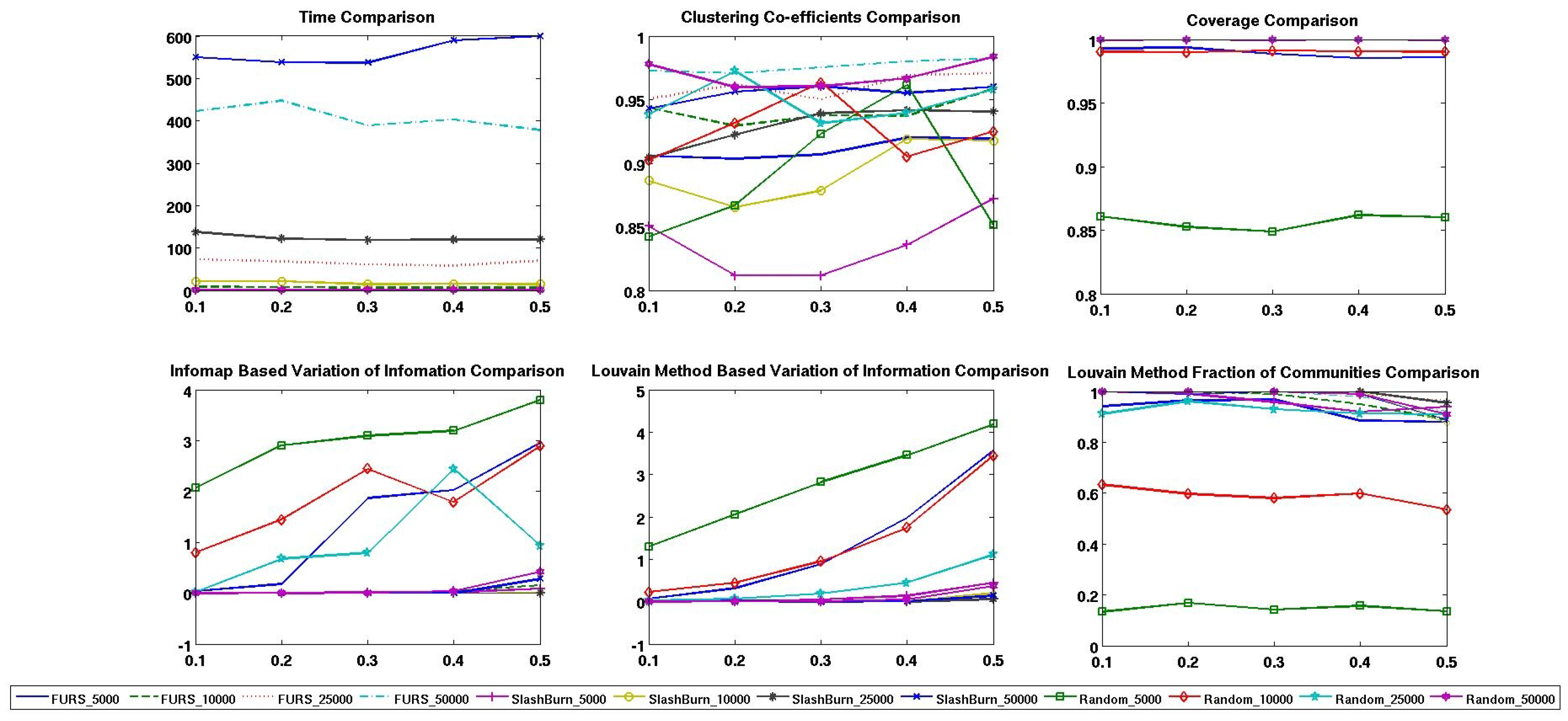
4.2. Comparison with other Techniques on Synthetic Networks

We also compare the FURS selection technique with SlashBurn and Random sampling methods on a variety of synthetic networks of increasing size and using multiple mixing parameters as depicted in Figure 5. These synthetic networks were also generated by the software provided by Fortunato as mentioned earlier. We maintain the size of the subset as 15 % of the nodes in the network based on experimental findings in [20] and set the k for “k-hubset” for SlashBurn as 0 . 5 % of the nodes as recommended in [18]. For the Infomap [7] and Louvain [9] community detection techniques, we evaluate the subset obtained by FURS on various metrics such as computation time, clustering coefficients (CCF), coverage, variation of information (VI). We also evaluate the ratio of the number of communities in the large network to the number of communities obtained in the subgraph for the different sampling techniques using Louvain method (fraction of communities preserved). These metrics and a bunch of other metrics are described in detail along with their evaluations on several community detection algorithms in [17].
In Figure 5 the lines determine the value of evaluation metrics like time required, clustering coefficient, coverage, variation of information and fraction of communities covered for each value of mixing parameter μ { 0 . 1 , 0 . 2 , 0 . 3 , 0 . 4 , 0 . 5 } . These lines correspond to 3 different sampling algorithms including the FURS selection, SlashBurn and Random sampling methods on synthetic networks containing 5 , 000 , 10 , 000 , 25 , 000 and 50 , 0000 nodes respectively. Several of these values are exactly the same and hence some of these lines completely overlap as observed from Figure 5. From Figure 5, we observe that Random sampling is the least expensive computationally but doesn’t preserve the original community structure. This can be observed from the variation of information (VI) for Louvain and Infomap method (lower values of VI are better) and also the fraction of communities preserved for Louvain method. Surprisingly, the coverage value turns out to be high for Random sampling except for networks with 5000 nodes. The SlashBurn algorithm is computationally expensive and doesn’t capture the CCF as well as FURS and Random sampling techniques. However, the SlashBurn approach is highly consistent w.r.t. the other evaluation metrics. The FURS selection technique is computationally less intensive than SlashBurn and better preserves the CCF. With the exception of synthetic networks with 5000 nodes, the FURS technique preserves the community structure of larger networks even with high mixing parameter as depicted in Figure 5. So, for large scale networks it is better to use the FURS selection technique.
Figure 5. Comparison of FURS, SlashBurn and Random sampling techniques for various evaluation metrics on synthetic networks with 5 , 000 , 10 , 000 , 25 , 000 , 50 , 000 nodes, with mixing parameter μ varying from 0 . 1 to 0 . 5 along the x-axis and the value of the metric plotted on the y-axis.
Entropy 15 01567 g005
We provide an algorithm that summarizes the KSC approach for big data networks in Appendix A.

5. Experiments and Analysis

We conducted experiments on several big datasets, including a synthetic network with 500 , 000 nodes, a social network with about 4 million nodes, a road network of city with around 2 million nodes, and YouTube network with more than 1 million nodes. These real world datasets are obtained from [26].

5.1. Dataset Description

  • Synthetic Network: The synthetic network is generated from the software provided in [6] with a mixing parameter of 0 . 1 . The number of nodes in the network is 500 , 000 , the number of edges in the network is 23 , 563 , 412 and the number of communities in the network is 6.
  • YouTube Network: In YouTube social network, users form friendship with each other and the users can create groups that others can join. This network has more than 1 million nodes and around 2 . 5 million edges. Thus the network is highly sparse.
  • roadCA Network: A road network of California. Intersections and endpoints are represented by nodes and the roads connecting these intersections are represented as edges. The number of nodes in the network is around 2 million and the number of edges in the network is more than 5 . 5 million.
  • Livejournal Network: It is a free online social network where users are bloggers and they declare friendship among themselves. The number of nodes in the network is around 4 million and the network has around 35 million edges.

5.2. FURS on these Datasets

We first apply the FURS technique on these datasets to select a training set and validation set of nodes. As mentioned earlier, the maximum number of nodes that we select using FURS selection technique is 5 , 000 nodes in order to have a kernel matrix that adheres to the memory restrictions. The step that we follow is to first select the training set using FURS, then these set of nodes are removed from the graph. We then run another iteration of FURS to select the validation set of nodes. Table 1 highlights the values of various evaluation metrics for these datasets for the FURS selection technique for the training set of nodes.
Table 1. Various evaluation metrics on FURS for each dataset.
DatasetNodesEdgesTimeCoverageClustering CoefficientDegree Distribution
Synthetic500,00023,563,412103.490.440.9060.786
YouTube1,134,8902,987,62420.5460.280.9750.959
roadCA1,965,2065,533,21430.8160.1350.890.40
Livejournal3,997,96234,681,189181.210.1730.920.953
From Table 1, we can observe that even after selecting just 5 , 000 nodes, which is equivalent to 0 . 01 , 0 . 0045 , 0 . 0025 , 0 . 00125 fraction of nodes in the four networks respectively, the coverage value is quite high. The clustering coefficient and degree distribution values have been converted into similarity metric as described in [16]. The maximum value for the clustering coefficient and degree distribution can be 1. Hence, the higher the value, the better the quality of the subset selected. We observe from Table 1 that these quality metrics have quite high values with the exception of 0 . 4 value of degree distribution for roadCA network. We also notice that the time required for subset selection for the Synthetic network is more than that for networks like YouTube and roadCA, which have more nodes. However, this is because the Synthetic network is much denser than these real world networks with around 23 million edges in comparison with nearly 2 . 5 and 5 . 5 million edges in the YouTube and roadCA networks respectively.

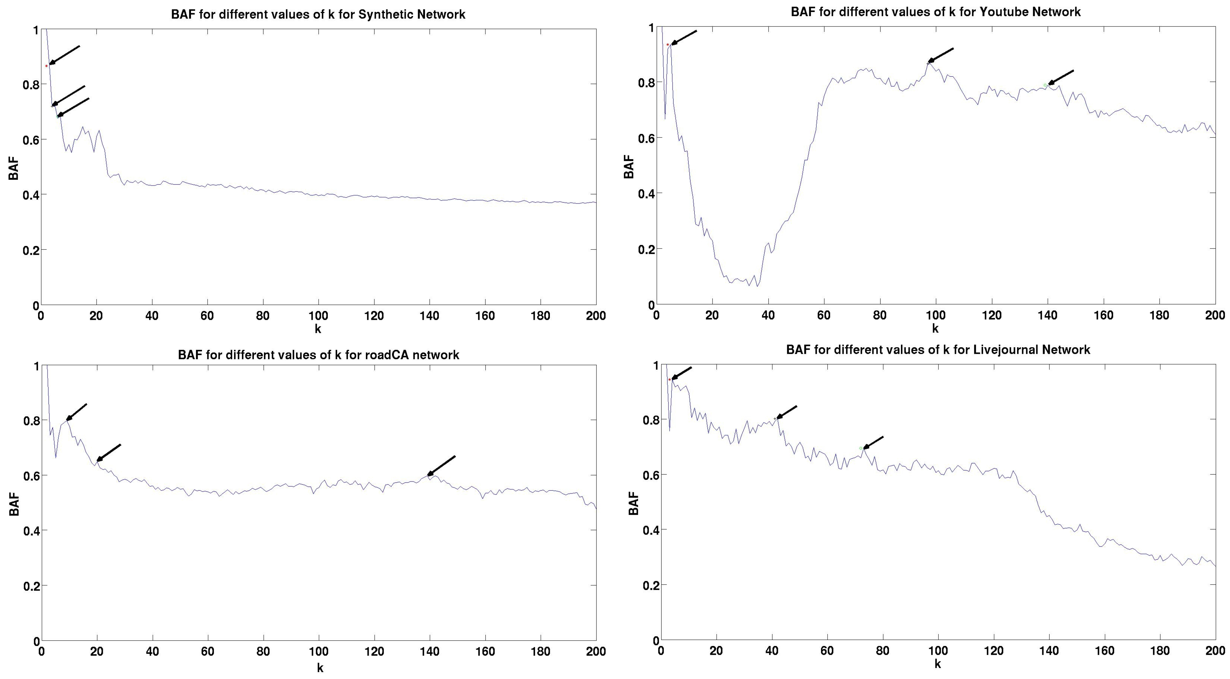
5.3. Results and Analysis

The kernel spectral clustering results in a model based on the subgraph selected by the FURS subset selection technique and uses its out-of-sample extension property to provide cluster labels for new unseen nodes. Since most of the spectral clustering methods, graph partitioning methods and graph clustering methods require to take into consideration the full network into the main memory, it would be unfair to compare KSC with these methods. There are several graph clustering techniques like Louvain method, Infomap method, CNM [4], which can scale up to million nodes on a single computer. However, if the size of the network increases such that it can no longer fit in the memory, then these methods would become infeasible.
Figure 6. B A F for different values of k for the various big data networks.
Entropy 15 01567 g006
Figure 6 shows the model selection or identification of the number of clusters k for the different datasets. We plot 3 dominant peaks for each of the 4 datasets. Currently, we select the peaks based on an adhoc procedure. We sort B A F values and select the maximum and restrict from selecting peaks in the immediate neighborhood as we might miss the hierarchical structure in that case. As mentioned earlier, the B A F metric is not only suitable for model selection but can also be used as an effective cluster evaluation metric. The higher the B A F value, the better the partitioning of the network. We observe that for the Synthetic network the B A F values are high for small number of clusters. Thus, in this case we make an exception and select the peaks close to each other. For the Synthetic network we do locate a peak at k = 6 with B A F = 0 . 6817 , which is the actual number of clusters present in the network. For the YouTube network, we observe that we reach the first dominant peak at k = 9 and then the B A F value starts to decrease before it starts to increase again and locates the next dominant peak at k = 97 . This shows the effectiveness of the B A F metric for identification of hierarchical structure in the big data network. For the YouTube network the B A F values decrease initially as the value of k increases indicating that the clusters are not well-formed. However, its value start to increase from k = 40 as we are now obtaining the second level of hierarchy. The B A F value is 0 . 8654 for k = 97 which indicates that there are 97 well partitioned clusters at the second level of hierarchy for the YouTube network. For the roadCA and Livejournal networks, the B A F generally follows a decreasing trend with the increment in the number of clusters with a few spurious dominant peaks as depicted in Figure 6. The maximum number of clusters in the network was fixed as 200 in our experiments and we observe that it is sufficient to provide a general trend for B A F versus the number of clusters (k) curve.
Table 2 provides details about three dominant peaks, time required for training, i.e., time required for building the kernel matrix and obtaining the model ( α ( l ) , b l ), validation time and the time required for testing. For testing, we use the entire big data network as test set. We noticed that it is not possible to store the big Ω t e s t in the main memory and we divided the test data into blocks containing adjacency list of maximum 5 , 000 nodes as described in Algorithm 2 in Appendix A. The maximum number of nodes we selected for training set is 5 , 000 , taking into account the memory constraints.
Table 2. Experimental results for various Big Data Networks
DatasetPeak 1 BAF 1 Peak 2 BAF 2 Peak 3 BAF 3 Train Time (Seconds)Validation Time (Seconds)Test Time (Seconds)
Synthetic30.860540.71960.6817103.45111.4210234.5
YouTube50.9348970.86541390.787788.6497.8620055.45
roadCA90.798200.64821380.591797.412105.1338960
Livejournal40.94355410.8014730.6951121.43134.5697221.4
From Table 2, we observe that the training time for building the model for these big data networks is quite small. The training time comprises of constructing the kernel matrix (Ω) and performing eigen-decomposition to obtain the model ( α ( l ) , b l ). The validation time comprises of creating Ω v a l i d , using out-of-sample extensions to obtain e v a l i d ( l ) and obtain the model parameter, i.e., the number of clusters k using the B A F metric. The maximum time required is the test time, i.e., time required to create Ω t e s t and cluster memberships using out-of-sample extensions for each block of the large network. We observe that the number of blocks into which the Synthetic network, YouTube network, roadCA network and Livejournal network are divided is 100, 227, 394 and 800 respectively. The average testing time for each block of each dataset is nearly the same as the time required for training the model for that dataset. The testing operation can easily be performed in a distributed environment. Thus, the time required for testing can be scaled down by a factor of 20–40 depending on the number of computers in the cluster of the distributed environment. We observe that the time required for training the Synthetic network is more than that of YouTube and roadCA networks, although they have more number of nodes. This is because the Synthetic network is much denser than these two real world datasets.
We also compare the proposed KSC method using BAF metric (BAF-KSC) with original KSC formulation using BLF criterion (BLF-KSC), Louvain, Infomap and CNM on evaluation metrics like Modularity (Q) and conductance (Con) for several small scale real world networks to provide a comparison of the performances. We have considered a wide range of networks varying from flight network (Openflights), network based on trust (PGPnet), biological network (Metabolic), citation networks (HepTh, HepPh), communication network (Enron), review based network (Epinion) to collaboration network (Condmat). Most of these networks can be found at [26].
Table 3. Performance comparison of BAF-KSC method with BLF-KSC, Louvain, Infomap and CNM methods on quality metrics like Modularity (Q) and Conductance (Con) for several real world networks.
DatasetBAF-KSCBLF-KSC [14]Louvain [9]Infomap [7]CNM [4]
ClustersQConClustersQConClustersQConClustersQConClustersQCon
Openflights50.5330.00250.5230.0021090.610.02180.580.005840.600.016
PGPnet80.580.00290.530.0021050.880.045840.870.031930.850.041
Metabolic100.220.02850.2150.012100.430.03410.410.05110.420.021
HepTh60.450.000450.4320.00041720.650.0041710.30.00460.4230.0004
HepPh50.560.000450.410.001820.720.007690.620.0660.480.0007
Enron100.40.00270.210.00112720.620.0510990.370.2760.250.0045
Epinion100.220.0003100.220.0330.0060.0003170.180.0002100.140.0
Condmat60.280.0002130.430.000310300.790.0310860.790.02580.380.0003
From Table 3 we observe that the BAF-KSC and BLF-KSC methods results in small number of clusters. This is because we consider the first peak corresponding to the highest B A F and B L F value respectively. We also observe that since the KSC method results in small number of clusters the conductance (Con) value is the quite low for most of the networks. The lower the conductance value the better the quality of the clusters. We also observe that the Modularity (Q) metric value is generally high for the BAF-KSC and BLF-KSC methods but less in comparison to Louvain method. We also observe the Q value is higher for the proposed KSC method (BAF-KSC) over the original KSC formulation (BLF-KSC) for 7 real world networks. Higher values of Modularity (Q) mean more modular graph partitions. The Louvain method is the best w.r.t. the Q metric as it optimizes the Modularity function. However, the conductance for the Louvain method for the various real world networks is generally 10 times more than the conductance for the KSC method. The CNM and BLF-KSC methods results in best conductance for Epinion networks as it identifies small number of well separated clusters for these networks.

6. Conclusions

In this paper we showed that the Kernel Spectral Clustering (KSC) method is a powerful tool for community detection in big data networks. While the problem of community detection has received a lot of attention in the past, the state-of-the-art approaches work under the assumption that the entire network can fit in the main memory. However, with the increasing amount of information, the size of the networks will only increase and big data networks may not necessarily fit in the main memory.
The KSC method employs an optimization based framework to construct the model, which has a very useful out-of-sample extension property. However, the model that is constructed should be such that it adheres to the memory restrictions. Therefore, there is a need to select a representative subgraph of the big data network on which the model can be built. We use the FURS selection procedure for this purpose. It selects nodes from different dense regions of the graph while maximizing the coverage and preserves the inherent community structure of the big data network.
In order to obtain the model parameters (i.e., the number of clusters k in the network in case of large complex networks), we propose a novel metric Balanced Angular Fit. The B A F metric works with a codebook CB and the projections of the validation set to determine the ideal number of clusters k in the big data network. The metric is both memory- and computationally efficient, unlike the previously proposed Modularity metric. The out-of-sample extensions property allows inferring community affiliation for unseen nodes. It is because of this property that we can handle large scale networks relatively easily. Finally, we show that the KSC method works effectively on a big Synthetic Network and several real world big data networks. Future work may focus on automatically determining the dominant peaks in B A F versus number of clusters curve.

Acknowledgements

This work was supported by Research Council KUL: ERC AdG A-DATADRIVE-B, GOA/11/05 Ambiorics, GOA/10/09MaNet, CoE EF/05/006 Optimization in Engineering (OPTEC), IOF-SCORES4CHEM, several PhD/postdoc and fellow grants; Flemish Government:FWO: PhD/postdoc grants, projects: G0226.06 (cooperative systems & optimization), G0321.06 (Tensors), G.0302.07 (SVM/Kernel), G.0320.08 (convex MPC), G.0558.08 (Robust MHE), G.0557.08 (Glycemia2), G.0588.09 (Brain-machine) G.0377.12 (structured models) research communities (WOG:ICCoS, ANMMM, MLDM); G.0377.09 (Mechatronics MPC) IWT: PhD Grants, Eureka-Flite+, SBO LeCoPro, SBO Climaqs, SBO POM, O&O-Dsquare; Belgian Federal Science Policy Office: IUAP P6/04 (DYSCO, Dynamical systems, control and optimization, 2007-2011); EU: ERNSI; FP7-HD-MPC (INFSO-ICT-223854), COST intelliCIS, FP7-EMBOCON (ICT-248940); Contract Research: AMINAL; Other:Helmholtz: viCERP, ACCM, Bauknecht, Hoerbiger.

References

  1. Schaeffer, S. Algorithms for Nonuniform Networks. PhD thesis, Helsinki University of Technology, Helsinki, Finland, 2006. [Google Scholar]
  2. Danaon, L.; Diáz-Guilera, A.; Duch, J.; Arenas, A. Comparing community structure identification. J. Stat. Mech. Theory Exp. 2005, 9, P09008. [Google Scholar] [CrossRef]
  3. Fortunato, S. Community detection in graphs. Phys. Rep. 2009, 486, 75–174. [Google Scholar] [CrossRef]
  4. Clauset, A.; Newman, M.; Moore, C. Finding community structure in very large scale networks. Phys. Rev. E 2004, 70, 066111. [Google Scholar] [CrossRef]
  5. Girvan, M.; Newman, M. Community structure in social and biological networks. Proc. Natl. Acad. Sci. USA 2002, 99, 7821–7826. [Google Scholar] [CrossRef] [PubMed]
  6. Lancichinetti, A.; Fortunato, S. Community detection algorithms: A comparitive analysis. Phys. Rev. E 2009, 80, 056117. [Google Scholar] [CrossRef]
  7. Rosvall, M.; Bergstrom, C. Maps of random walks on complex networks reveal community structure. Proc. Natl. Acad. Sci. USA 2008, 105, 1118–1123. [Google Scholar] [CrossRef] [PubMed]
  8. Langone, R.; Alzate, C.; Suykens, J.A.K. Kernel spectral clustering for community detection in complex networks. In Proceeding of the IEEE International Joint Conference on Neural Networks (IJCNN), Brisbane, Austrilia, 10–15 June 2012; pp. 1–8.
  9. Blondel, V.; Guillaume, J.; Lambiotte, R.; Lefebvre, L. Fast unfolding of communities in large networks. J. Stat. Mech. Theory Exp. 2008, 10, P10008. [Google Scholar] [CrossRef]
  10. Ng, A.Y.; Jordan, M.I.; Weiss, Y. On Spectral Clustering: Analysis and an Algorithm. In Proceedings of the Advances in Neural Information Processing Systems; Dietterich, T.G., Becker, S., Ghahramani, Z., Eds.; MIT Press: Cambridge, MA, USA, 2002; pp. 849–856. [Google Scholar]
  11. Von Luxburg, U. A tutorial on spectral clustering. Stat. Comput. 2007, 17, 395–416. [Google Scholar] [CrossRef]
  12. Zelnik-Manor, L.; Perona, P. Self-tuning Spectral Clustering. In Advances in Neural Information Processing Systems; Saul, L.K., Weiss, Y., Bottou, L., Eds.; MIT Press: Cambridge, MA, USA, 2005; pp. 1601–1608. [Google Scholar]
  13. Shi, J.; Malik, J. Normalized cuts and image segmentation. IEEE Trans. Pattern Anal. Intell. 2000, 22, 888–905. [Google Scholar]
  14. Alzate, C.; Suykens, J.A.K. Multiway spectral clustering with out-of-sample extensions through weighted kernel PCA. IEEE Trans. Pattern Anal. Mach. Intell. 2010, 32, 335–347. [Google Scholar] [CrossRef] [PubMed]
  15. Newman, M.E.J. Modularity and community structure in networks. Proc. Natl. Acad. Sci. USA 2006, 103, 8577–8582. [Google Scholar] [CrossRef] [PubMed]
  16. Maiya, A.; Berger-Wolf, T. Sampling Community Structure. In WWW ’10, Proceedings of the 19th International Conference on World Wide Web, Raleigh, NC, USA, 26–30 April 2010; pp. 701–710.
  17. Mall, R.; Langone, R.; Suykens, J.A.K. FURS: Fast and Unique Representative Subset Selection for Large Scale Community Structure; Internal Report 13–22; ESAT-SISTA, K.U.Leuven: Leuven, Belgium, 2013. [Google Scholar]
  18. Kang, U.; Faloutsos, C. Beyond ‘Caveman Communities’: Hubs and Spokes for Graph Compression and Mining. In Proceedings of 2011 IEEE 11th International Coference on Data Mining (ICDM), Vancouver, Canada, 11–14 December 2011; pp. 300–309.
  19. Metropolis, N.; Rosenbluth, A.; Rosenbluth, M.; Teller, A.; Teller, E. Equation of state calculations by fast computing machines. J. Chem. Phys. 1953, 21, 1087–1092. [Google Scholar] [CrossRef]
  20. Leskovec, J.; Faloutsos, C. Sampling from large graphs. In Proceedings of the 12th ACM SIGKDD International Conference on Knowledge Discovery and Data Mining, Philadelphia, USA, 20–23 August 2006; pp. 631–636.
  21. Langone, R.; Alzate, C.; Suykens, J.A.K. Kernel spectral clustering with memory effect. Phys. Stat. Mech. Appl. 2013, 392, 2588–2606. [Google Scholar] [CrossRef]
  22. Chung, F.R.K. Spectral graph theory (CBMS regional conference series in mathematics, No. 92). Am. Math. Soc. 1997. [Google Scholar]
  23. Suykens, J.A.K.; van Gestel, T.; de Brabanter, J.; de Moor, B.; Vandewalle, J. Least Squares Support Vector Machines; World Scientific: Singapore, Singapore, 2002. [Google Scholar]
  24. Muflikhah, L. Document clustering using concept space and cosine similarity measurement. In Proceedings of International Conference on Computer Technology and Development (ICCTD), Kota Kinabalu, Malaysia, 13–15 November 2009; pp. 58–62.
  25. Baylis, J. Error Correcting Codes: A Mathematical Introduction; CRC Press: Boca Raton, FL, USA, 1988. [Google Scholar]
  26. Stanford Large Network Dataset Collection Home Page. Available online: http://snap.stanford.edu/data/ (accessed on 3 May 2013).

Appendix A

Entropy 15 01567 i002

