1. Introduction
Entropy generation mechanisms play key roles in determining the second-law irreversibility in energy-conversion processes in internal combustion (IC) engines and gas turbines. Fundamental understanding of entropy generation mechanisms is pivotal to the efficient design of new generation IC engines and gas turbines. For this purpose, it is important to understand local behaviour of the different entropy generation mechanisms. Bejan [
1] analysed the entropy generation mechanisms due to viscous action and heat transfer in channel flows. Local entropy generations due to heat and mass transfers in addition to viscous effects have been analyzed by San
et al. [
2] and Poulikakos and Johnson [
3]. Puri [
4] analyzed entropy generation in the context of droplet combustion and identified the optimum transfer number for the purpose of minimization of entropy generation. Hiwase
et al. [
5] subsequently proposed a theoretical model for exergy analysis for droplet-laden flows where the exergy loss is expressed as a function of Damköhler number and initial droplet temperature. Exergy analysis in spray combustion was analyzed by Datta and Som [
6] for different conditions in terms of pressure, temperature, swirl number, droplet diameter and spray cone angle. Arpaci and Selamet [
7] analyzed entropy generation in laminar premixed flames on a flat flame burner using analytical means and expressed the entropy generation rate in terms of the quenching distance. Nishida
et al. [
8] analysed entropy generation mechanisms in laminar hydrogen-air and methane-air premixed flames based on detailed chemistry based simulations and demonstrated the effects of equivalence ratio on the entropy generation in premixed flames. Different mechanisms of entropy generation in multi-component reacting systems have been identified in a number of previous analyses [
8,
9,
10,
11,
12,
13,
14,
15] on premixed and non-premixed combustion. Interested readers are referred to [
15] for an extensive review of entropy generation in reactive system. It has been found that viscous dissipation, thermal conduction, mass diffusion and irreversible chemical reaction give rise to generation of entropy in reacting flows.
To date, most analyses on local entropy generation mechanism have been carried out for laminar flows [
7,
8,
10,
11,
12,
13,
14] and relatively limited effort was given to the entropy generation mechanism in turbulent flames [
14,
15,
16,
17]. OKong’o and Bellan [
16] and Safari
et al. [
17] discussed the importance of the local entropy transport in the context of combustion modelling especially for Large Eddy Simulations (LES). The present analysis is carried out following the theoretical basis provided by Safari
et al. [
17], but the statistical behaviors of the entropy generation mechanisms in response to the variations of combustion regime, heat release parameter and global Lewis number in turbulent premixed flames were not addressed in [
17]. However, these effects have been adequately addressed in this paper based on the analysis of Direct Numerical Simulations (DNS) data of statistically planar turbulent premixed flames.
In last two decades DNS has become an important tool for the analysis of turbulent flows where all the relevant length and time scales associated with turbulent flow processes are simulated without any recourse to physical approximations. Analysis of local entropy generation in turbulent flames based on DNS data has rarely been done in the existing literature. This void has been addressed here by analyzing entropy generation mechanisms in turbulent premixed flames based on three-dimensional compressible DNS data. As the nature of the fuel and the equivalence ratio of the mixture have significant influences on the entropy generation in turbulent premixed flames [
8], a systematic parametric analysis based on DNS simulations has been carried out in this paper for different values of heat release parameter
and global Lewis number
(as the equivalence ratio, nature of the fuel and the level of preheating can be characterized by
and
). The heat release parameter
and global Lewis number
are defined as follows:
where
,
,
,
,
and
are the adiabatic flame temperature, unburned gas temperature, thermal conductivity, gas density, specific heat at constant pressure and the mass diffusivity respectively. Moreover, turbulent flow conditions may have an influence on the entropy generation in turbulent premixed flames. Thus a DNS database of freely propagating statistically planar turbulent premixed flames with a range of values of heat release parameters
(ranging from 2.3 to 4.5) and global Lewis numbers
(ranging from 0.34 to 1.2) spanning both the corrugated flamelets and the thin reaction zones regimes, has been considered to analyze the different entropy generation mechanisms in turbulent premixed combustion. In this respect, the main objectives of the present investigation are as follows:
- (1).
To analyze the relative contributions of viscous dissipation, heat conduction, mass diffusion and chemical reaction towards the overall entropy generation in turbulent premixed combustion.
- (2).
To identify the effects of combustion regime, heat release parameter and global Lewis number on the different entropy generation mechanisms in turbulent premixed flames.
The rest of the paper will be organized as follows: the details related to the mathematical background and numerical implementation will be presented in the next two sections. Following this, results will be presented and subsequently discussed. Main findings will be summarized and conclusions will be drawn in the final section of this paper.
2. Mathematical Background
The volumetric rate of destruction of exergy in turbulent premixed flames due to irreversibilities can be expressed as:
where
is the unburned gas temperature (which is considered to be the dead state in this analysis) and
is the volumetric rate of entropy generation which can be obtained from the transport equation of entropy. The transport equation of entropy takes the following form [
7,
8,
9,
10,
11,
12,
13,
14,
15,
16,
17]:
where
,
,
,
,
,
and
are the temperature, internal energy, pressure, density, specific volume, specific chemical potential of species
(per unit mass and not in terms of unit mole) and the mass fraction of species
respectively. The specific chemical potential
is given by:
where
is the specific enthalpy of species
,
is the reference temperature,
is the specific heat at constant pressure for species
,
is the partial specific entropy which is given by:
where
and
are the number of moles and molecular mass of species
respectively and
denotes the extensive entropy. Here all the species are considered to be ideal gases and for ideal gases
can be expressed as:
where
,
and
are the mole fraction, specific entropy and gas constant of the pure species
with
being the universal gas constant. Using Equations. (2)–(6) the entropy transport equation takes the following form:
where
is the reaction rate for species
, which is negative (positive) for a reactant (product). The components of viscous stress tensor
and the
i-th components of heat flux vector
and mass flux vector
are expressed using the Newton’s law of viscosity, Fourier’s law of heat conduction and Fick’s law of mass diffusion respectively, in the following manner:
where
is the viscosity,
is the
i-th component of velocity,
is the thermal conductivity,
is the mass fraction of species
and
is the mass diffusivity of species
. It is worth noting that Soret and Dufor effects are ignored here following several previous analyses on entropy generation in turbulent reacting flows [
4,
5,
6,
7,
8,
10,
11,
12,
13,
14,
15,
17]. Moreover, there have been several previous DNS based computational analyses [
18,
19,
20,
21,
22,
23,
24,
25,
26,
27,
28,
29,
30,
31,
32,
33,
34], which ignored Dufor and Sorret effects without much loss of generality. These effects are not expected to play important roles in most hydrocarbon-air and hydrogen-air flames [
35] unless extremely lean hydrogen-air flames are considered. Moreover, it is worth noting that this analysis follows the theoretical basis provided by Safari
et al. [
17], which also ignored Soret and Dufor effects. Equation (8) can be utilised to recast Equation (7) as:
For ideal gas the derivative of Equation (5) takes the following form:
where the last term on the right hand side is often neglected for low Mach number flows [
7,
8,
9,
10,
11,
12,
13,
14,
15,
16,
17] and thus Equation (11) can be used in Equation (10) to yield:
Thus, the last term on right hand side of Equation (9) can be expressed as:
Here specific heats and mass diffusivities of all the species are taken to be identical (
i.e.,
and
), which leads to:
Using Equations (12) and (14) in Equation (9) yields:
where:
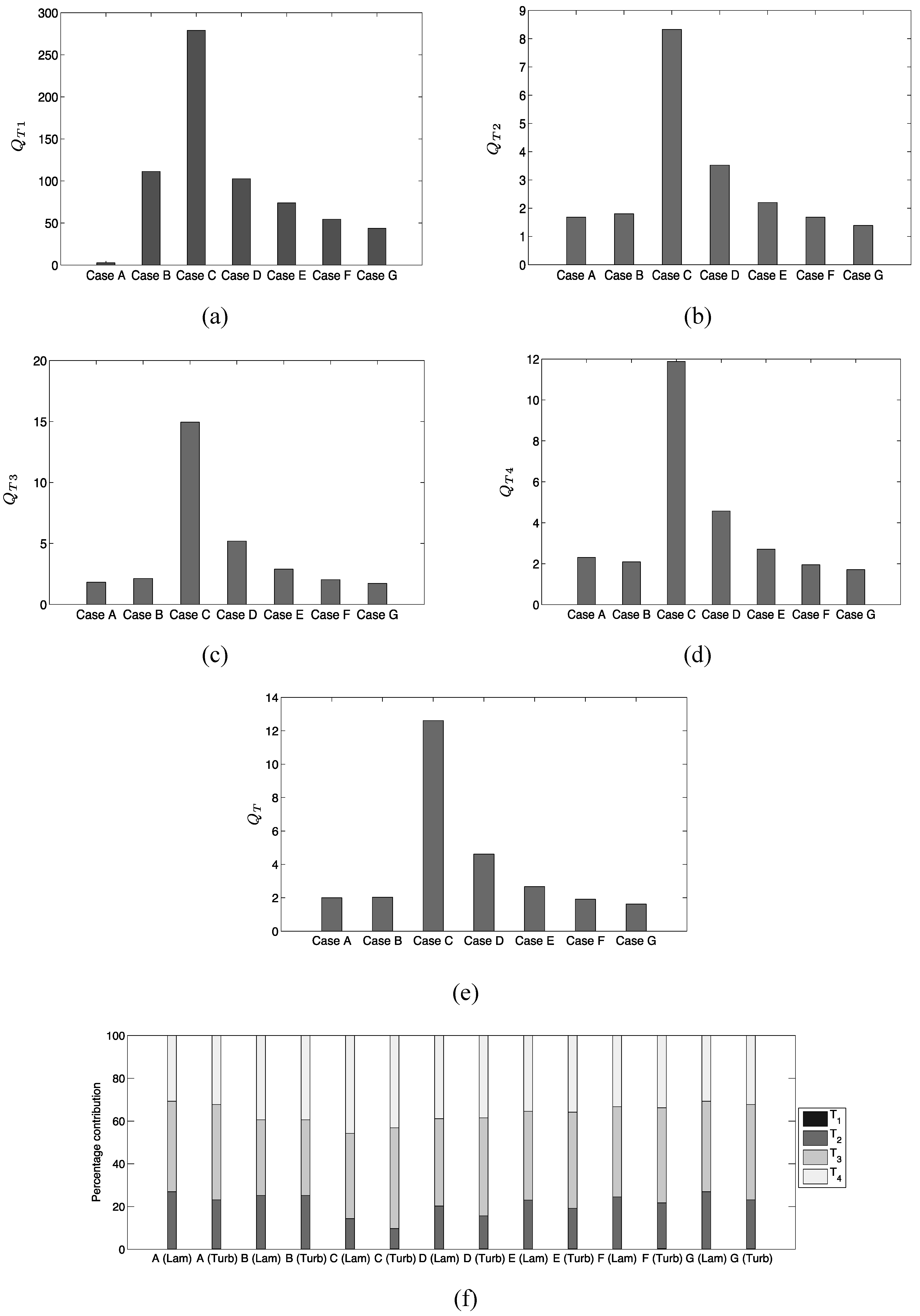
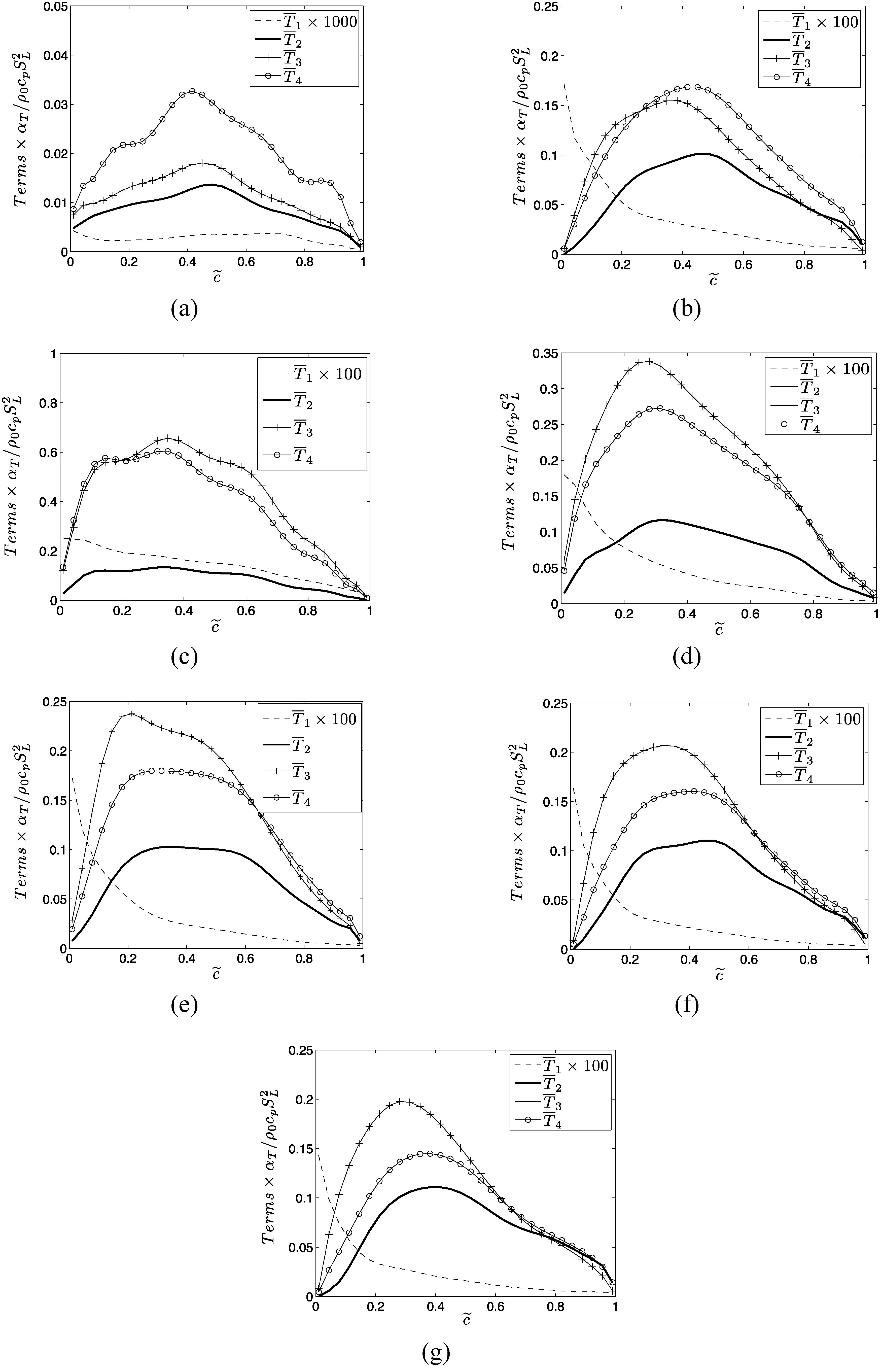
The terms
and
denote entropy generation due to viscous action, chemical reaction, thermal conduction, and mass diffusion respectively. The volumetric rate of entropy generation is given by:
The second term on right hand side of Equation (15i) is identically zero for unity Lewis number cases (i.e., ). For non-unity Lewis number cases (i.e., ) is responsible for redistributing entropy and the volume integral of this term vanishes according to divergence theorem (i.e., where and are elemental surface area and volume respectively and is the outward normal on the elemental surface) because vanishes both on unburned and burned gas sides of the flame brush.
The extent of augmentation of entropy generation rate due to viscous dissipation in turbulent flames can be quantified by using a quantity
which is defined as:
The subscripts “turb” and “lam” are used to refer to the values in turbulent and laminar flames respectively. Similarly, the augmentation of entropy generation rate due to
,
and
in turbulent conditions in comparison to the corresponding laminar flames can be characterized by
and
, which are defined as:
Based on Equations (17)–(20) the overall augmentation of entropy generation in turbulent flames in comparison to the corresponding laminar flames can be characterized as:
Ideally DNS of turbulent premixed combustion should account for both three-dimensionality of turbulence and detailed chemical mechanism. However, until recently most combustion DNS simulations were carried out either in two-dimensions with detailed chemistry or in three-dimensions with simplified chemistry due to limitations in computer storage capacity. The CPU time for compressible DNS of turbulent reacting flows scales as:
where
is the turbulent Reynolds number,
is the Karlovitz number,
is the number of grid points within the thermal flame thickness
,
is the number of large-scale eddies within the domain and
is the number of eddy turn-over times, where the subscript
L refers to the unstrained planar laminar flame quantities. The value of
remains of the order of 10 and 20 for simple chemistry and detailed chemistry based DNS simulations respectively. Moreover, one needs to have
to obtain enough number of statistically independent turbulent velocity signals and
in order to ensure that the simulation results are independent of initial conditions. This suggests that detailed chemistry simulations, for a given set of values of
and
, are several orders of magnitude more expensive than simple chemistry simulations, especially for hydrocarbon-air flames (e.g., 68 steps and 18 species are typically involved in detailed chemistry based methane-air flame simulations). Although three-dimensional DNS with detailed chemistry is becoming possible using multi-processor simulations [
36], they still remain prohibitively expensive [
36,
37] for an extensive parametric analysis, as carried out in this paper. Thus the chemical mechanism is simplified here using a generic single-step Arrhenius type chemical reaction (
i.e.,
) and the three-dimensionality of turbulence is simulated without any physical approximation. Single step chemistry has been used successfully to obtain fundamental physical insight and to develop high-fidelity models in several analyses in the past [
18,
19,
20,
21,
22,
23,
24,
25,
26,
27,
28,
29,
30,
31,
32,
33,
34] and the same methodology has been followed here. In the context of simplified chemistry the species field is characterized by a reaction progress variable
, which can be defined in terms of a suitable reactant mass fraction
as follows:
where subscripts
and
denote the values in pure reactants and fully burned products. In the context of single step chemistry the term
takes the following form as
:
where subscripts P and R refer to quantities for products and reactants respectively. The difference between chemical potentials between products and reactants (
i.e.,
) can be expressed as:
In the present analysis the generic chemical mechanism is taken to represent typical hydro-carbon/hydrogen-air combustion where the number of moles does not change significantly as a result of chemical reaction. For such chemical reactions
remains almost same as
(
i.e.,
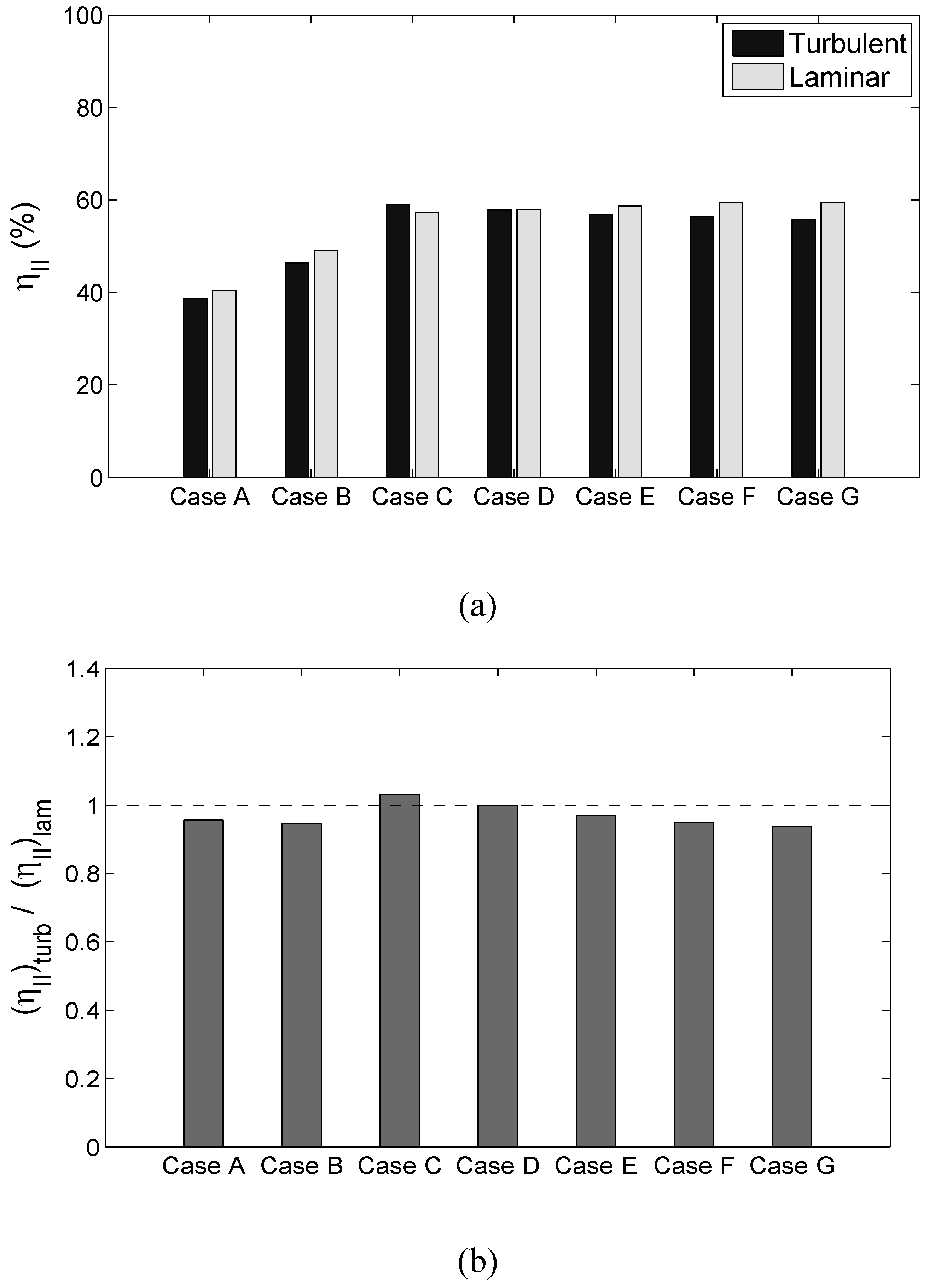
) under globally adiabatic conditions. Based on the above theoretical background, the extent of irreversibility in turbulent premixed combustion can be expressed in the form of second-law efficiency
which can be defined in the following manner:
The effects of combustion regime, heat release parameter and global Lewis number on the statistical behaviors of
and
will be discussed in detail in
Section 4.2 of this paper.
It is important to note that the statistics of flame propagation and scalar gradient in turbulent premixed flames based on simple chemistry DNS are found to be in good agreement with the corresponding two-dimensional detailed chemistry DNS results (
i.e.,
. flame propagation statistics for simple chemistry DNS in [
21,
33] are in agreement with detailed chemistry DNS results in [
38,
39]; statistical behaviors of scalar gradient obtained from simple chemistry DNS in [
24,
40,
41] are in agreement with detailed chemistry based results in [
42,
43,
44] and [
41] respectively). A comparison between References. [
23] and [
42] (see
Figure 3a in [
23] and
Figure 1a in [
42]) indicates that the variation of
with
obtained from single-step Arrhenius type chemistry is qualitatively similar to detailed chemistry based results for methane-air and hydrogen-air flames. It is worth noting that the simulations considered here mimic generic hydrocarbon-air flames (
e.g., methane-air flames) for
cases, whereas
and 0.6 cases represent hydrogen-air/hydrogen-blended hydrocarbon-air combustion. In actual combustion process a change in equivalence ratio/fuel-type alters the values of heat release parameter
and global Lewis number
. Moreover, the level of pre-heating also affects the value of heat release parameter
. It is worth noting that the global Lewis number
is modified here independently of the other parameters for the purpose of identifying the effects of differential diffusion of heat and mass in isolation. However, it is difficult to assign a single characteristic Lewis number in a reacting flow field due to the presence of several species with different Lewis numbers. Often the Lewis number of deficient species is considered to be the global Lewis number characterizing the combustion process [
35,
45]. There have seen several studies in the past where the effects of differential diffusion of heat and mass have been analyzed by modifying the global Lewis number in isolation [
18,
19,
20,
21,
22,
23,
24,
25,
26,
46,
47,
48].The same approach has been adopted in this analysis. Equation (15ii) indicates that the entropy generation in premixed flames is dependent on the statistics of reaction rate
and scalar gradients
,
and
, and as the statistics of reaction rate and scalar gradients are adequately captured by single-step chemistry, it can be expected that fundamental features of entropy generation in turbulent premixed flames can also be addressed using simple chemistry. The effects of regime of combustion,
and
on local entropy generation due to
and
will be analyzed in detail in
Section 4 of this paper.
3. Numerical Implementation
In the present study a DNS database of freely propagating statistically planar turbulent premixed flames under decaying turbulence has been considered. The initial values for the root-mean-square (rms) turbulent velocity fluctuation normalized by unstrained planar laminar burning velocity
and the integral length scale to flame thickness ratio
are presented in
Table 1 along with the values of Damköhler number
(i.e. the ratio of the integral time-scale
to the chemical time-scale
), Karlovitz number
, turbulent Reynolds number
, heat release parameter
and Lewis number
. Standard values are taken for Prandtl number
, ratio of specific heats
and the Zel’dovich number
(
i.e.,
,
,
). The thermo-chemical parameters for cases A–G are chosen in such a manner so that the thermal diffusivity of the unburned gas
, specific heat at constant pressure
, unstrained laminar burning velocity
and unburned gas density
remain the same for all cases considered here. It can be seen from
Table 1 that the turbulent Reynolds numbers are comparable for all the cases considered here. The simulation domain is taken to be a rectangular parallelepiped of size
(
) for case A (cases B-G), which is discretized by a Cartesian grid of
(
) with uniform grid spacing in each direction. Each 230 × 230 × 230 simulation required approximately 2300CPU-hours using AMD Opteron 2214 2.2Ghz CPU processors and approximately 50 Gb per case for storage. In all cases the
-direction is taken to align with the direction of mean flame propagation, whereas the other directions are considered to be periodic. The domain boundaries in the
-direction in case A are taken to be turbulent inlet and outlet respectively. The domain boundaries in the direction of mean flame propagation in other cases are taken to be partially non-reflecting. The partially non-reflecting boundaries are specified using the Navier Stokes Characteristic Boundary Condition (NSCBC) technique [
49]. According to NSCBC technique, the inviscid part of the Navier Stokes equations are specified using a characteristic analysis based on a locally one-dimensional system
(for
i = 1–5) where
,
,
,
and
, and the wave velocities
are given by
,
and
with
being the local acoustic speed. The wave amplitude variations
directed into the domain need to be specified at the partially non-reflecting boundaries and the wave amplitude variations for the outgoing waves are estimated from internal solutions. For the incoming waves the following expressions for
s :
,
,
,
and
were considered, where
and
are the target values of
and
respectively and
s are the relevant relaxation parameters [
49]. The values of
(for
j= 1, 2 and 3) ,
and
are considered to be zero at the partially non-reflecting boundaries [
49], where
and
are the heat and mass fluxes respectively. Interested readers are referred to [
49] for a more detailed discussion on boundary conditions.
In case A, the spatial differentiation in the
-direction is carried out using a 6th order central difference scheme for the internal grid points but the order of the differentiation gradually deceases to one-sided 4th order difference scheme as the non-periodic boundaries are approached, whereas the differentiation in the transverse directions are carried out using a spectral method. For the other cases, a 10th order central-difference scheme is used for spatial discretisation for internal points in all directions which gradually decreases to a one-sided 2nd order scheme near non-periodic boundaries. The time advancement for all viscous and diffusive terms in case A is carried out using an implicit solver, whereas the convection terms in case A and all the terms in all other cases are time advanced using a low-storage third order Runge-Kutta method [
50]. For all cases, the flame is initialized by a steady unstrained planar laminar flame solution, and the turbulent velocity fluctuation field is specified using an initially homogeneous isotropic field generated using a pseudo-spectral method [
51]. The grid spacing is determined by the resolution of the flame structure, and about 10 grid points are kept within the thermal flame thickness
for all cases considered here. Case A represents the corrugated flamelets regime combustion (
i.e.,
) [
52], whereas other cases represent the thin reaction zones regime combustion (
i.e.,
) [
52]. The values of heat release parameter
are different for cases A, B and C-G. The Karlovitz number can be taken to scale as [
52]:
where
is the Kolmogorov length scale. Equation (26) suggests that the energetic turbulent eddies cannot penetrate into the flame in the corrugated flamelets regime combustion, whereas turbulent eddies are likely to penetrate into the preheat zone in the thin reaction zones regime combustion. However, the Kolmogorov length scale
remains greater than the reaction zone thickness in the thin reaction zones regime combustion so that chemical reaction can be sustained.
In all cases flame-turbulence interaction takes place under decaying turbulence. Under decaying turbulence, simulations should be carried out for at least
, where
is the initial eddy turn over time and
is the chemical time scale. The simulation in case A was run for about four initial eddy turn over times
, whereas simulations were run for a time
in cases B–G. The aforementioned simulation times remain either greater than (cases A) or equal to (cases B–G) one chemical time scale and are comparable to several previous analyses [
18,
19,
20,
21,
22,
23,
24,
25,
26,
27,
28,
29,
30,
31,
32,
33,
34,
35,
38,
39,
40,
41,
42,
43,
44]. The turbulent kinetic energy and its dissipation rate in the unburned gas ahead of the flame were not varying significantly with time when statistics were extracted and the qualitative nature of the statistics was found to have remained unchanged since
for all cases. The values of
in the unburned reactants ahead of the flame at the time when statistics were extracted decreased by about 52% and 50%, of the initial values in cases A and B-G respectively. The values of
have increased from their initial values by a factor of about 1.10 and 1.7 for cases A and B-G respectively, but there are still enough number of turbulent eddies on each side of the computational domain.
In
Section 4 the Reynolds averaged values of
and
will be presented. For statistically planar flames the Reynolds/Favre averaged quantities are considered to be functions of the distance along the direction of mean flame propagation (
direction), and are evaluated by ensemble averaging the relevant quantities in transverse directions (
planes). The statistical convergence of the Reynolds/Favre averaged quantities are assessed by comparing the corresponding values obtained using half of the sample size in the transverse directions using a distinct half of the domain, with those obtained based on full sample size. Both qualitative and quantitative agreements between these sets of values are found to be satisfactory. In the next section, only the results obtained based on full sample size will be presented for the sake of brevity.
Table 1.
List of initial turbulence and combustion parameters for the present DNS database.
Table 1.
List of initial turbulence and combustion parameters for the present DNS database.
| Case | | | | | |
|---|
| A | 1.41 | 9.64 | 56.7 | 6.84 | 0.54 |
| B-G | 7.5 | 2.45 | 47.0 | 0.33 | 13.17 |
| Le = 1.0 (A, B, F) 0.34 (C),0.6 (D), 0.8 (E) and 1.2 (G). 2.3 (A), 3.0 (B), 4.5 (C–G) |
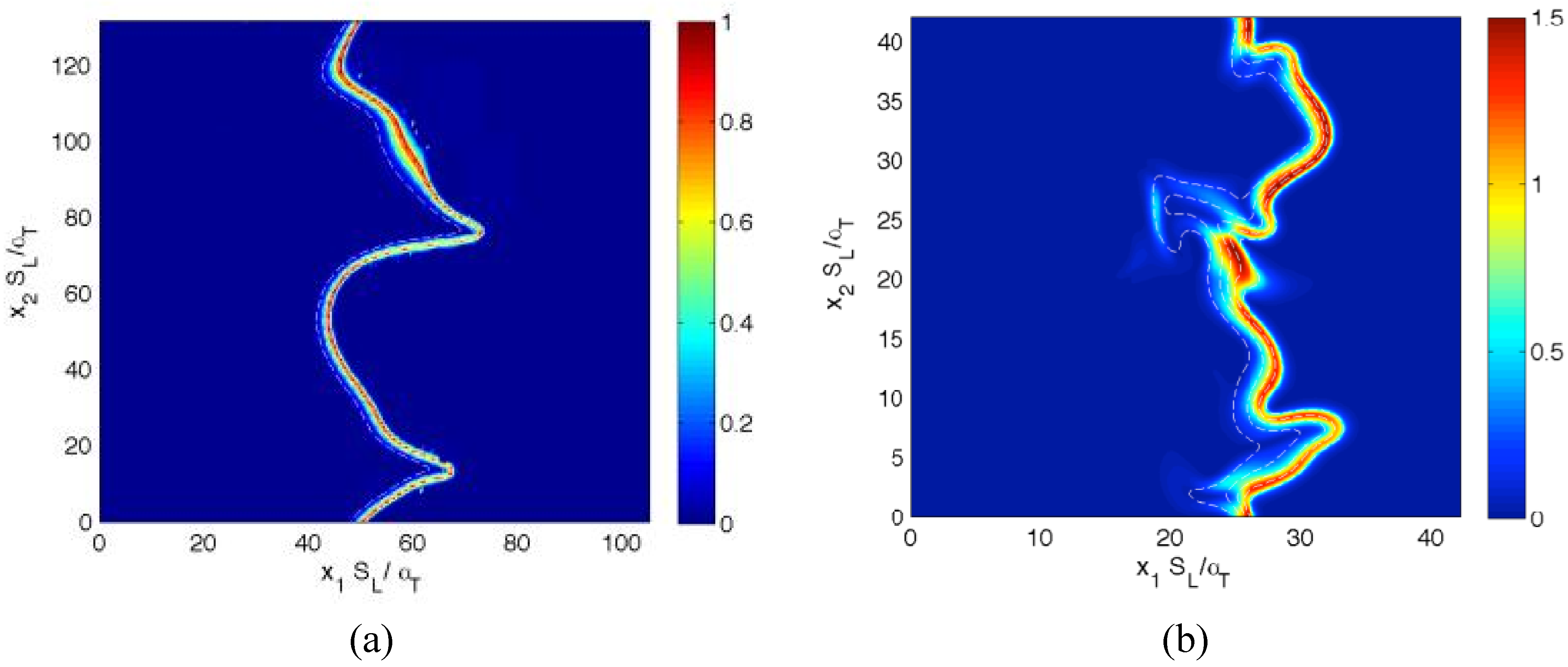
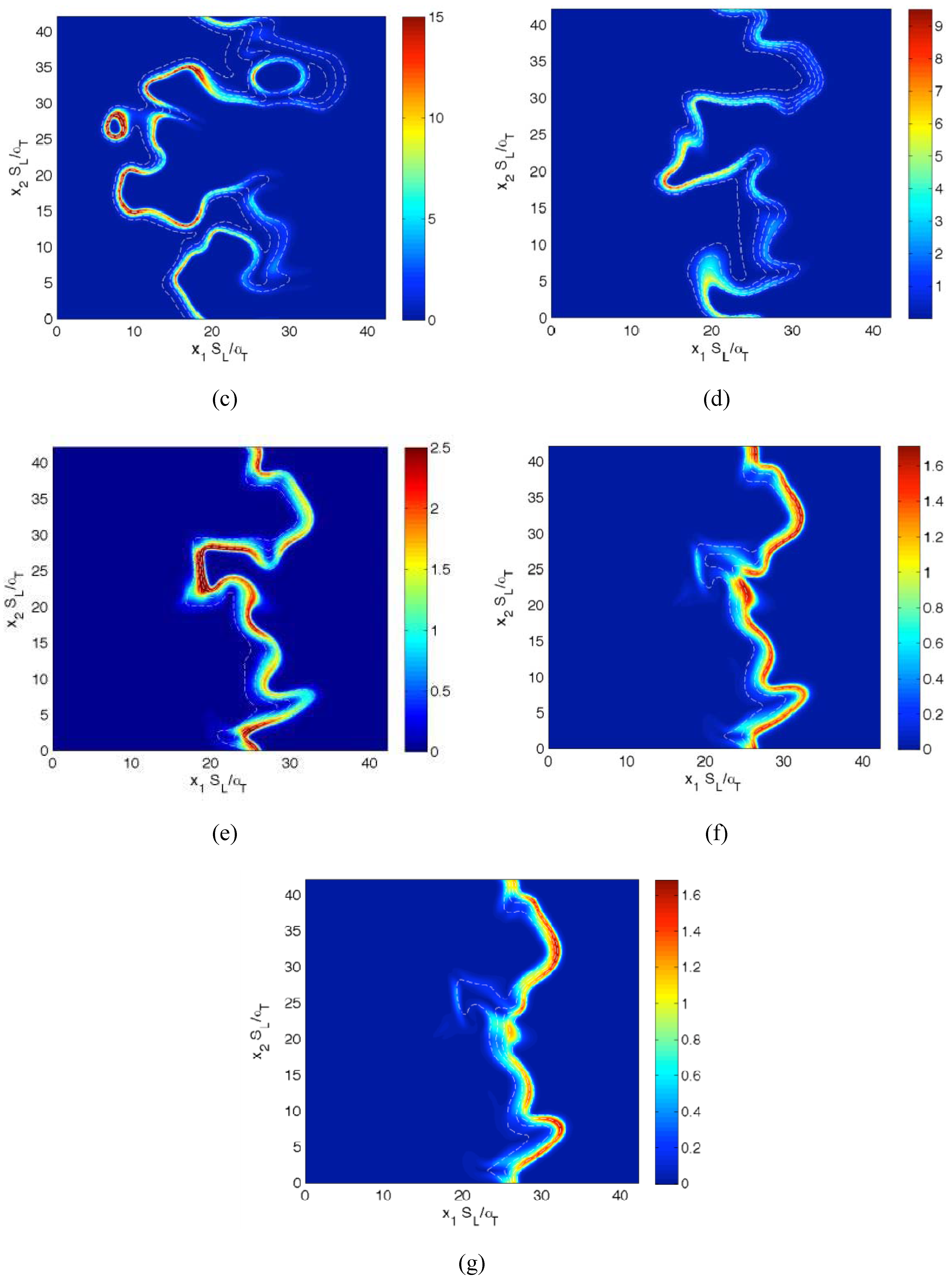
Figure 1.
Distributions of in the central plane for cases (a–g) A–G at the time when the statistics were extracted. The white lines indicate reaction progress variable c contours from c = 0.1 to 0.9, from left to right, in steps of 0.2.
Figure 1.
Distributions of in the central plane for cases (a–g) A–G at the time when the statistics were extracted. The white lines indicate reaction progress variable c contours from c = 0.1 to 0.9, from left to right, in steps of 0.2.
5. Conclusions
Different mechanisms of entropy generation in turbulent premixed flames have been analyzed in detail based on a simple chemistry DNS database with a range of different values of heat release parameter , global Lewis number spanning both the corrugated flamelets and thin reaction zones regimes of combustion. It has been found that the entropy generation increases under turbulent conditions. It has been found that the regime of combustion does not significantly affect the augmentation of entropy generation due to chemical reaction, thermal conduction and mass diffusion in turbulent flames in comparison to the corresponding laminar flames, whereas the entropy generation in turbulent flames due to viscous dissipation in comparison to the corresponding laminar flames is stronger in the thin reaction zones regime than in the corrugated flamelets regime. However, the regime of combustion does not significantly affect , as viscous dissipation plays a marginal role in the overall entropy generation in premixed flames. The global Lewis number has been found have a profound influence on the entropy generation mechanism due to thermal conduction, chemical reaction and mass diffusion and the entropy generation by all the aforementioned mechanisms strengthen with decreasing . By contrast, significantly affects the entropy generation mechanism due to thermal conduction but other entropy generation mechanisms are marginally influenced. The entropy generation mechanism by the viscous dissipation remains negligible in comparison to the entropy generations due to chemical reaction, thermal conduction and mass diffusion for both laminar and turbulent conditions. Detailed physical explanations have been provided for the observed trends of entropy generation mechanisms in response to the changes in and . The enhancement of entropy generation rate under turbulent conditions is superseded by the augmentation of burning rate for flames and thus the second law efficiency for turbulent and 0.6 flames are found to be either greater than (for ) or comparable to () the corresponding laminar flame values. By contrast, enhancement of entropy generation rate overcomes the augmented burning rate under turbulent conditions, which in turn leads to smaller value of for turbulent flames, than in the corresponding laminar flames. Thus, a trade-off between heat release and second-law efficiency will be necessary for choosing an ideal fuel-air composition for a new industrial burner.
It is worth noting that this analysis has been carried out in the context of simplified chemistry and transport. The entropy generation in premixed flames is dependent on the statistical behaviors of reaction rate
and scalar gradients
,
and
, and as the statistics of reaction rate and scalar gradients are adequately captured by single-step chemistry (see comparison between References. [
23] and [
42] for reaction rate statistics between simple and detailed chemistry; comparison between References. [
21,
33] and [
38,
39] for flame propagation statistics between simple and detailed chemistry; comparison between References. [
24,
40,
41] and [
41,
42,
43,
44] for scalar gradient statistics between simple and detailed chemistry) it can be expected that the present findings based on simplified chemistry will be at least qualitatively valid in the context of detailed chemistry based analysis. However, the quantitative prediction of entropy generation for each individual case is likely to be different due to the effects of detailed chemistry and transport on
. Thus, further analysis with detailed chemistry and transport will be necessary for more comprehensive DNS based analysis of entropy generation mechanisms in turbulent premixed combustion.


