Abstract
Persistent misconceptions existing for dozens of years and influencing progress in various fields of science are sometimes encountered in the scientific and especially, the popular-science literature. The present brief review deals with two such interrelated misconceptions (misunderstandings). The first misunderstanding: entropy is a measure of disorder. This is an old and very common opinion. The second misconception is that the entropy production minimizes in the evolution of nonequilibrium systems. However, as it has recently become clear, evolution (progress) in Nature demonstrates the opposite, i.e., maximization of the entropy production. The principal questions connected with this maximization are considered herein. The two misconceptions mentioned above can lead to the apparent contradiction between the conclusions of modern thermodynamics and the basic conceptions of evolution existing in biology. In this regard, the analysis of these issues seems extremely important and timely as it contributes to the deeper understanding of the laws of development of the surrounding World and the place of humans in it.
Keywords:
Prigogine’s principle; Ziegler’s principle; applicability of MEPP; Jaynes’s maximization; biological evolution PACS Codes:
05.70.Ln; 87.23.-n
1. Thermodynamic Entropy and Disorder. Is there a Difference in the Evolution of Animate and Inanimate?
The notion of entropy (S) was introduced into science by R. Clausius (1822–1888) in 1850–1865. According to his studies, the change of entropy can be written as:
where δQ is the heat obtained (given) by the system at the (absolute) temperature T in the quasi-equilibrium process.
The statement of the fact that a macroscopic system has a single-valued function of state (the entropy, S) constitutes the essence of the second law of thermodynamics. It can be shown (see, for example, [,]) that entropy defines irreversible dissipation of energy, and processes in an isolated system always occur with the non-reduction of entropy.
The entropy notion is used primarily for deductive development of an important branch of theoretical physics: thermodynamics. The complexity of this notion consists in the fact that we are unable to immediately feel or perceive entropy (as, for instance, temperature, body coordinates, or pressure). The value of entropy can be defined only indirectly by measuring, for example, the thermal capacity for the isochoric process CV and then calculating it based on the formula:
where TX is the temperature in the state X in which the absolute value of the entropy SX is determined. In order to find the absolute value of entropy, e.g., according to Equation (2), another postulate, the third law of thermodynamics (at T ° 0, the entropy tends to zero), needs to be introduced.
In 1877, L. Boltzmann (1844–1906) first pointed out the possible relationship between the thermodynamic entropy and the microscopic properties of matter:
where k is some constant and Ω is the number of possible microstates (different arrangements of a system) corresponding to the macroscopic state of the system.
The Equation (3) is very important for further discourse. Therefore, we shall show its use based on the simplest example (Figure 1). Let us consider a vessel divided into two sections. We shall place two particles in one section. Thus, the first state has been prepared. Obviously, this state can be created in only one way. So, Ω1 = 1. Let us assume that the particles can move (diffuse) freely in the vessel. Obviously, the system will reach the second macroscopic state. This state can be implemented in three equiprobable ways (see Figure 1), and therefore Ω2 = 3. According to Equation (3), the second state will show higher entropy as compared to the first state. This agrees with the second law: an isolated system changes from some prepared (nonequilibrium) state to the equilibrium state and the entropy increases. Obviously, the second state (Figure 1) is more disordered than the first one as the particles can be located in one part of the vessel or the other at different moments of time.
The examples similar to the one analysed above and Boltzmann’s statistic interpretation of entropy Equation (3) gave rise to an opinion that the notion of entropy is related to the notion of disorder. According to the second law of thermodynamics, the entropy grows in the nonequilibrium isolated system; then, in line with the mentioned relation, the disorder should also grow. In contrast, most theories of the origin and development of life on Earth state that all living organisms (see []) become more complex and organized with time and, consequently, tend to be more and more distant from chaos (become ordered). This contradiction appeared in the beginning of the XXth century and created a barrier between physics, which then dealt mainly with inanimate matter, and the science of animate, i.e., biology. As a consequence, this period is marked by rebirth and development of the vitalism concept, which states a drastic difference between the phenomena of life and the physical and chemical phenomena. The vitalists believe that the development of living organisms is primarily caused by some nonmaterial supernatural power: “vital force” (“entelechy”) according to the German biologist H. Driesch (1867–1941), “vital impulse” according to the French philosopher H. Bergson (1859–1941), and the like.
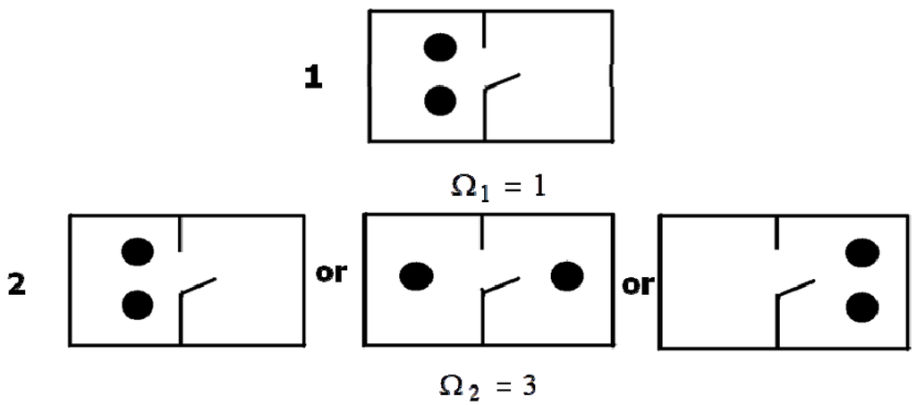
Figure 1.
The simplest model explaining the notion of microstate.
The study by E. Schrödinger (1887–1961) [], the renowned Austrian physicist, is the first, the most interesting and cited (up until now) attempt to solve the formulated problem. Let us comment on his point of view. The change of the entropy S (or, for the unit volume, s) with the time t is the sum of the entropy generation (production) in a body Σ (or, for the unit volume, the entropy production density σ) and the total entropy flux () entering or leaving through the boundary (Π) of the body under consideration:
or, for the unit volume (locally):
According to the second law, Σ (or σ) is always above zero; however, the second summand Equations (4*) and (4**) can have a considerably higher value, and then the total change of entropy dS/dt will be negative. As a consequence, the entropy of the body at hand will decrease. Let us note that the total entropy of the whole isolated system (the body with the surrounding environment) will not go down in complete agreement with the second law of thermodynamics. If entropy is viewed as a measure of disorder, then the body in the above example will mostly give the contained disorder to the environment rather than receive it from the outside or produce it internally. As a result of this exchange, the order inside the body increases. It is important to note that, according to Schrödinger, only the animate can have this property, and the inanimate has no such ability. The proposed mechanism of the entropy reduction and the Equation (4) provoke no objections. However, the division between the animate and inanimate systems based on their ability to “absorb order” from the environment (if it was really true) does not eliminate but, on the contrary, creates a barrier between the animate and the inanimate. Indeed, it is stated that the animate systems have some exclusive properties (qualitative differences), the special physics. Let us quote []: “New laws to be expected in the organism.”
As further experiments and analysis showed, the conclusion that the animate systems have an exclusive nature in terms of the entropy outflow value was premature. Starting from the middle of the twentieth century, an enormous number of examples of the inanimate systems’ self-organization (formation of dissipative structures) was studied (see, for example, [,]). As a result of the research that still continues today, the scientists concluded that the main condition for the emergence of structures from homogeneous (chaotic) environment is: the openness and the sufficient nonequilibrium state of the system. Thus, the conflict between the animate and the inanimate caused by the study [] turns out to be imaginary.
However, is the above question connected with the difference in evolution of the animate and inanimate systems from the perspective of the entropy and disorder behavior finally solved? Obviously, no! Let us adduce two arguments. The first argument: animate systems continuously become more complex over time (e.g., the evolution from protozoans to mammals). This is true both under varying and, what is the more important, under constant external conditions (e.g., in the case of approximately the same chemical composition of the environment and equal energy received from the Sun). Inanimate systems have no such property and quickly finish “generation” of new structures; such systems reach the stationary state and thus end their evolution under invariable external parameters (for instance, the degree of nonequilibrium). Therefore, the question of what forces the life to continuously develop and become more complex remains. The second argument: the study of the self-organization process using Equation (4) is speculative in the majority of cases and not supported by calculations (which are absent, for instance, in [,,] and in multiple other much more recent publications related to the subject). Considering entropy as a measure of disorder, it is believed that the entropy undoubtedly decreases in the case of the emergence of a structure (for example, the Benard cell) or the evolution from unicellular organisms to humans because a less disordered, more highly organized structure appears. The absence of quantitative calculations of the thermodynamic entropy and its change during the self-organization is connected with the extreme complexity of such calculations due to considerable spatial and temporal inhomogeneity and the nonequilibrium state of such systems. This makes it necessary to introduce multiple assumptions, which influences the accuracy and significantly reduces the value of the result.
In view of the latter, we cannot but mention a widely known and cited study by L. Blumenfeld [], where he evaluates the thermodynamic entropy change during of the construction of an organism from cells, the cells from biopolymers, and the biopolymers from monomers. The calculation was performed only for the configuration part of entropy, while the interaction between the constituent “bricks” of the system was neglected. Obviously, the value obtained by such calculation is a very rough estimate of the thermodynamic entropy for which the second law of thermodynamics is formulated and the Equations (1), (2) and (4) are written. In spite of this drawback, Blumenfeld’s conclusion seems correct and very important. Let us quote it []: “All talks about “antientropic tendencies” of the biological evolution, about the exclusive order of the animate matter are based on an evident misunderstanding. According to the thermodynamic criteria, any biological system is ordered no more than a lump of rock of the same weight.”
This conclusion is confirmed by the data given in [] and obtained more rigorously by calculating exactly the thermodynamic entropy. So, under normal conditions, the entropy of one kilogram of wood (pine or oak) was 2.8 kJ/K. If we compare this value to the entropy of the "inanimate bodies" that surround the tree and have the same mass, the calculated entropy can be both higher (for instance, as compared to 0.7 kJ/K, the entropy of quartz SiO2, one of the most common minerals on Earth) and lower (for instance, as compared to 3.9 kJ/K or 6.8 kJ/K, the entropy of water and air, respectively).
Thus, the thermodynamic entropy is very difficult to find for animate systems and it cannot be used for distinguishing between the animate and inanimate matter. The above values suggest that the entropy can hardly be employed for the calculation of the degree of disorder in the real bodies during their self-organization. However, is it just a consequence of the fact that the occurring reduction in entropy during self-organization is negligible as compared with the absolute value of entropy, or is there other reasons?
The answer lies in the fact that the quantity of entropy is in no way related to the quantity of order observed during the self-organization (for instance, in the case of the appearance of the Benard cells) or the structure formation in biology. The immediate connection between the order and the entropy is an evident misunderstanding appeared in the beginning of the twentieth century and still encountered mostly in philosophical, biological and popular-science literature. The fact is that the physicists or chemists studying entropy and non-experts in this subject mean different concepts when speaking about “order”. For non-experts, the “order” of the structure is the systematicness, correctness in the arrangement. This is the “general-use” meaning. For physicists and chemists, the “order” of the structure is evaluated based on the complexity of prediction, which is related specifically to the number of microstates (Ω). The higher Ω (and, correspondingly, the higher the entropy, Equation (3)), the harder it is to predict the real location of the system. For non-experts, the “order” of the structure is estimated only in the real (spatial) three-dimensional space. The interaction between the parts of the structure is not taken into any consideration. For experts, the “order” of the structure and the entropy is calculated in the coordinate-momentum 6N-dimensional phase space. In addition, the interaction is explicitly taken into account in the Hamiltonian used for the calculation of the entropy. The interaction significantly influences the phase volume available to the system (and Ω). The mentioned points were to some extent formulated in the literature before (see, for example, [,,,]); however, they are largely left unheeded by the main addressees, the scientists who use the notion and the properties of the thermodynamic entropy and at the same time consciously and unconsciously identify the entropy with the order in “their” (rather than the conventional physical) understanding.
We also have to make an important remark that has served and still serves as a source of the misunderstanding under discussion. So, as follows from the above, if the evolution of almost non-interacting particles in the three-dimensional space is considered (assuming that the particle velocity distribution has already been established), then the change of order/disorder calculated by a physicist (a chemist) will qualitatively agree with non-experts’ understanding of the order/disorder variation. In a certain sense, this is the case when studying the spatial behaviour of an ideal gas. The ideal gas model was introduced by R. Clausius and used by L. Boltzmann in the discussion of entropy (see Figure 1 as an example). In our opinion, this was a key moment in the confusion (identification of the thermodynamic entropy with the order in the general-use meaning rather than in the specific physical one) that started more than a hundred years ago and can still be encountered today.
As can be seen from the above, the thermodynamic entropy is a more complex notion than a measure of spatial disorder. Consequently, the thermodynamic entropy increase and the order increase during the biological evolution or other self-organization process cannot be compared.
However, the above question still remains: what forces the life to continuously develop and become more complex, and can this question be solved within the scope of thermodynamics? Can it be true that the supporters of Schrödinger and Blumenfeld, who believe that the problems of origin and evolution of biological structures are beyond the scope of physics because its laws are insufficient for understanding thereof, are right? In our opinion, it is not the physics of “animate” that is required but a deeper investigation of the properties of entropy and, first of all, the rate of its change: entropy production.
2. Entropy Production. Direction of the Evolution of Inanimate and Animate Systems
The nonequilibrium processes in nature are very often described using the so-called linear nonequilibrium thermodynamics. The foundation thereof was laid by L. Onsager (1903–1976) in 1931. By theoretically generalizing the empirical laws (of G. Ohm, A. Fick, J. Fourier, and others), he proposed a linear relationship between the thermodynamic fluxes Ji (particularly, the heat flux) and the thermodynamic forces Xi (particularly, the temperature gradient):
and grounded the reciprocal relation for the kinetic coefficients :
These equations form the basis of the linear nonequilibirium thermodynamics. They are used to close and solve the system of energy-, momentum-, and mass-transfer equations. It is important to note that the simplest linear Equations (5) may prove to be incorrect for some nonequilibrium process (e.g., chemical reactions or some mechanical deformations), and the non-linear relations between the thermodynamic fluxes and forces have to be used.
It can be easily shown (see, for example, [,]) that the entropy production density (see Equation (4)) is related to Ji and Xi as follows:
Whereas the entropy is an essential quantity in the equilibrium thermodynamics, the entropy production assumes this role in the nonequilibrium thermodynamics. This was partially caused by two principles connected with the entropy production.
2.1. Prigogine’s and Ziegler’s Principle
The first statement was formulated in 1945–1947 by I. Prigogine (1917–2003). This statement was called a principle (or a theorem) of the minimum entropy production. It is formulated as follows [,]:
Let the main Equations of the linear nonequilibrium thermodynamics (5) and (6) be realized in a system, and a part of the total number of the thermodynamic forces Xi, be maintained constant, then the minimum entropy production density shall be the necessary and sufficient condition for the stationary state of the nonequilibrium system.
Generally, there are two points considered as the main drawbacks of this principle (see, for example, [,]). The first drawback: the principle is valid only for the linear nonequilibrium thermodynamics. The second drawback is more important. The principle is not constructive as the information required for its application should be so complete that the principle does not add anything new; and it is, as a rule, much easier to solve the problem directly using the laws of conservation and Equations (5) and (6) than using Prigogine’s principle. The minimum principle (theorem) was proved as a local (differential) statement. However, there were attempts to use this principle for finding the spatial distribution of physical quantities (i.e., to extend the application of the principle to the so-called integral case) (see, e.g., []). Nevertheless, such an extended understanding of the principle is, for the most part, wrong (see, for example, []).
Despite the mentioned drawbacks, the minimum entropy production principle still attracts a lot of attention among scientists, especially biologists and philosophers. This was contributed, on the one hand, by high reputation of the author and his popularization activity, and, on the other hand, by the above atavism fixated in the minds of many people that “entropy is a measure of disorder”. As a result, there is an erroneous assumption that a nonequilibrium system tends to the minimum disorder production with time, which has something in common with some biological and social evolution ideas. The Prigogine paper [] that assumes the Equations (5) and (6) to be valid for biological systems and concludes that the continuous reduction of entropy production density occurs in the course of the biological development also contributed to rise of interest in the principle among biologists (see, for example, [,,,,]). It is known that the entropy production in the system is directly related to the rate of its heat production. So, the assumption of the decrease of σ can be reduced to the statement that the continuous reduction of specific (referred to the unit of weight) heat production (which is proportional to the intensity of oxygen consumption because oxidation processes are the supplier of energy for all reactions occurring in animate aerobic organisms) should take place during the development, growth, and ageing of animals and humans. The analysis of the existing data [,,] showed the decrease of oxygen consumption rate or specific heat production during the ontogenesis of different animals. However, it turned out to be that (see [,,,,,]) the increase of entropy production density is observed at the initial stages of the ontogenesis. In view of the above as well as the fact that the Equation (5) is too rough for the chemical reactions taking place in the animate systems, the application of the minimum entropy production principle to the study of the evolution of animate beings can be considered unreasonable. Let us also note that if Prigogine’s principle is assumed as the defining principle for the development of the animate, then the main aim of the animate’s individual development would be the soonest death (in this case, the entropy production reaches its minimum value: zero), not to mention the phylogenesis, which would be far too difficult to explain!
The second statement connected with the entropy production was formulated by H. Ziegler (1910–1985) in 1963. This is the maximum entropy production principle, which, at first glance, seems an antipode to the principle considered above. Ziegler’s principle is formulated as follows [,]: if the thermodynamic forces Xi are preset, then the true thermodynamic fluxes Ji satisfying the side condition (7) give the maximum value of the entropy production density σ(J). Mathematically, this principle can be written using the Lagrange multiplier µ in the form:
By varying the entropy production in terms of thermodynamic fluxes with constant forces, the following relationship between the fluxes and forces can be obtained from (8):
As can be seen from Equation (9), the relationship between the thermodynamic fluxes and forces can be both linear and nonlinear. This is an important corollary of Ziegler's principle. For ( is the coefficient matrix), the main Equations of the linear nonequilibrium thermodynamics (5) and (6) can be easily obtained from Equation (9). By introducing additional restrictions, the Prigogine theorem can be derived from Equations (5) and (6). Thus, the range of applicability of the Prigogine principle is much narrower than that of the Ziegler principle.
There is sometimes a misunderstanding of how one and the same entropy production can be both maximum and minimum. The reason lies in the constraints used in the entropy production variation: they are substantially different. The geometrical interpretation of this fact for the case of two fluxes and is given in Figure 2. In Ziegler’s method (Figure 2a), the entropy production density is maximized for the fluxes , at the cross-section of the paraboloid by the plane perpendicular to the vectors with the components (this plane is positioned angle-wise to the ordinate axis). In Prigogine’s method (Figure 2b), the entropy production density is minimized for at the cross-section of the same paraboloid by the plane parallel to the ordinate axis (the plane equation is ). As a result of the extremization, the Ziegler method allows finding a relationship between the thermodynamic fluxes and forces (Equation (9) or Equations (5), (6) for the particular form of considered in Figure 2), whereas the Prigogine method (where Equations (5) and (6) are postulated) allows finding that the equation corresponds to the minimum entropy production density. The Ziegler and Prigogine variations can occur consequently in time for the same system. Indeed, let us assume that the thermodynamic forces are constant during some interval of time τ0. Then, based on Ziegler's principle, the system will adjust its thermodynamic fluxes in order to maximize the entropy production. If the entropy production is a quadratic function, then such an adjustment will result in the linear relationship between the fluxes/forces, and the system will reach its stationary nonequilibrium state. If the behavior of this system is considered for longer (than τ0) times τ, then a number of thermodynamic forces can become free (varying). In this case, the fluxes formed according to Ziegler (Equations (5) and (6)) will start decreasing the thermodynamic forces, which, in turn, will reduce the fluxes and so on. As a result, the minimum entropy production is reached. Thus, some hierarchy of processes can be seen: for small times, the system maximizes the entropy production with the fixed forces and, as a result, the linear relations between the fluxes and forces become valid; for a large scale of time, the system varies the free thermodynamic forces in order to reduce the entropy production [].
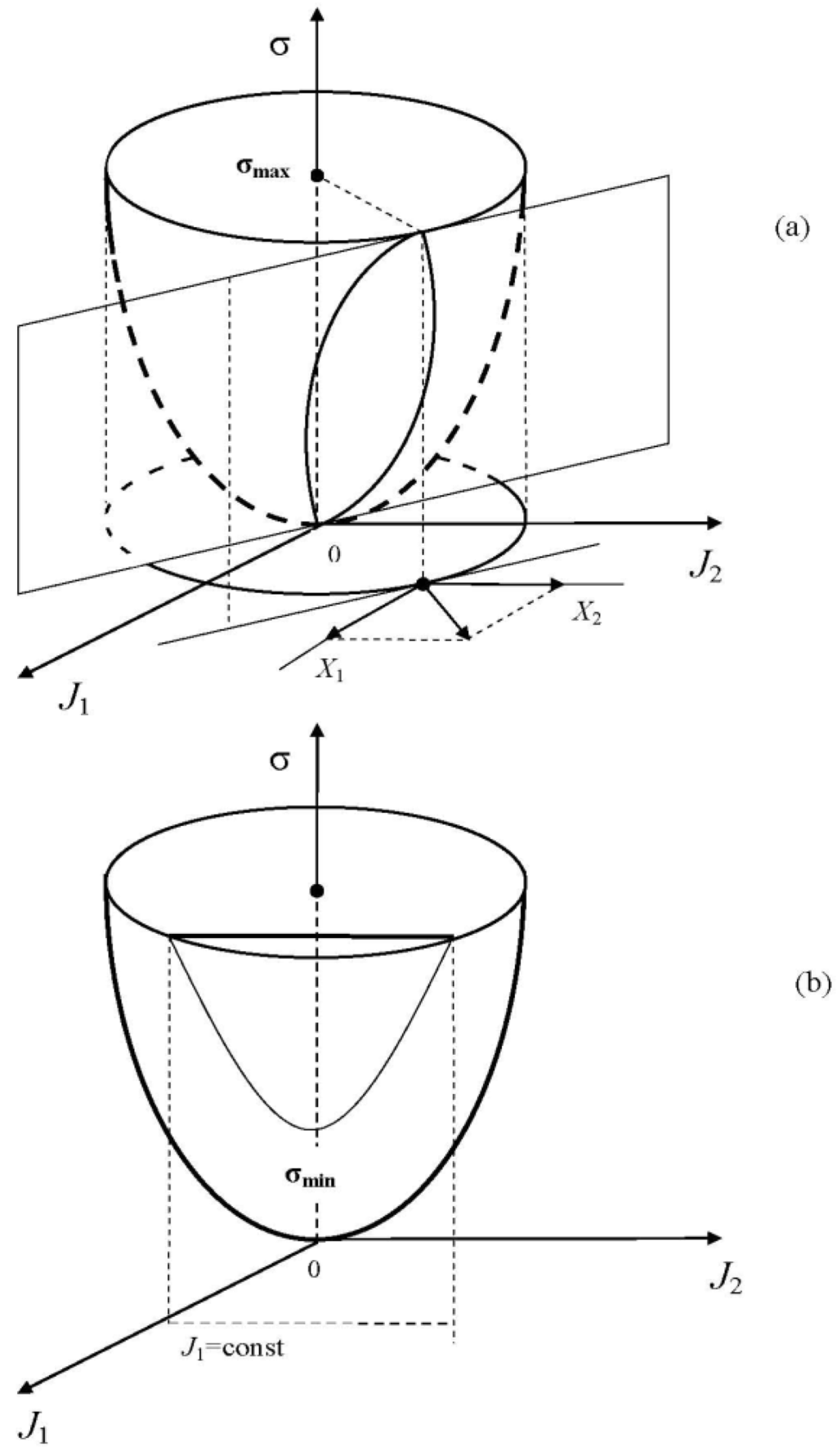
Figure 2.
Geometrical interpretation of the principles of Ziegler (a) and Prigogine (b) for the case of two thermodynamic fluxes (forces) in the system. In the first graph, the maximum entropy production on the plane positioned angle-wise to the ordinate axis is sought for; and in the second graph, the minimum entropy production on the plane parallel to the ordinate axis is sought for.
2.2. Maximum Entropy Production Principle (MEPP)
As can be seen from the above, the maximum entropy production principle is a more common statement than the minimum principle. However, as opposed to Prigogine’s principle, this principle failed to attract much attention. This is connected with the fact that H. Ziegler considered his principle only from the theoretical perspective within the scope of the nonequilibrium thermodynamics, applied it mainly for solving the problems of plasticity, and paid no attention to the popularization of his approach. Since the nonequilibrium thermodynamics theory also has other principles formulated for the nonlinear case, and the theory of plasticity also has other effective methods for solving the problems, Ziegler’s method basically remained unnoticed. However, the fact that statements similar to Ziegler’s principle were independently in different times and in different fields of science introduced by researchers for solving the arising problems (see multiple examples in [,]) places special emphasis on the importance of the Ziegler method. Let us give a number of examples demonstrating it.
- (1)
- There is a well-known variation method of solving the linearized Boltzmann equation used in the study of the transfer in gases, metals, and semiconductors. It is less known that M. Kohler [] and J. Ziman [] showed the identity of this variation method with the following statement: the velocity distribution function for nonequilibrium gas systems is such that the entropy production density is a maximum at preset gradients of the temperature, the concentration and the mean velocity. There are generalizations of this statement that are valid both for the quantum systems and for the relatively dense systems [,].
- (2)
- Based on the analysis of a large amount of empirical data, M. Berthelot [] formulated the following statement: if several chemical reactions can take place in a system without exposure to an external energy, the reaction, which is accompanied by the release of the largest heat, is realized. It can be shown [] that for a very wide range of chemical processes (especially at relatively low temperatures) the amount of heat produced by the reaction per unit of time is directly proportional to the entropy production. Therefore, the observations of Berthelot can be viewed as a kind of experimental confirmation of the maximum entropy production principle.
- (3)
- Based on the Rayleigh-Bernard convection data, W. Malkus [] assumed the statement: if the Rayleigh number is preset, the regime providing the maximum heat transfer (or in this case, the entropy production [,]) is realized among the multitude of possible stationary regimes of the transfer.
- (4)
- By analyzing the experimental and theoretical data of the nonequilibrium crystallization, D. Temkin [], J. Kirkaldy [], E. Ben-Jacob [], etc. assumed that, in the case of the fixed supersaturation/supercooling, the growing dendrite will select the maximum possible rate. As is known (see, for example, [,]), the entropy production density of the system under consideration is proportional to the squared growth rate of the crystal. Therefore, the presented data is indicative of the maximum entropy production principle.
There are other similar examples [,]. It is important that all statements were introduced: (1) independently; (2) for different systems and different scales (and levels) of description; (3) are reduced to the maximum entropy production principle; (4) demonstrate effectiveness in the solution of problems. All of the above made it possible for us to propose a generalized formulation of the maximum entropy production principle (MEPP) applicable to different scales of description [,]: at each level of description, with preset external constraints, the relationship between the cause and the response of a nonequilibrium system is established in order to maximize the entropy production density.
The maximum entropy production principle can be used in a variety of fields. Let us enumerate only some of them. In physics, G.P. Beretta [] and S. Gheorghiu-Svirschevski [] derive a nonlinear extension of the nonrelativistic Liouville-von Neumann dynamics on the basis of the maximum entropy production (steepest entropy ascent); P. Chavanis, et al. [] obtained a generalized relaxation equation of the Fokker-Planck type for modeling the movement of the galaxies; and, for instance, T. Christen [] modeled an electrical discharge in the gas far from equilibrium and obtained good estimates for the parameters of the system taking into account a number of nonlinear effects. In geophysics, G. Paltridge [,,] obtained the average annual distribution of temperature, heat fluxes, and cloudiness on Earth, which agreed well with the observations; and, for example, R. Lorenz et al. [] used MEPP to explain the anomalies of weather on Mars and Titan. In biology and ecology, A. Kleidon [] successfully applied the principle to study the role of biota in the exchange of carbon dioxide near the Earth surface; and, for instance, D. Juretić, et al. [] modeled the stationary photosynthesis of bacteria.
The accumulated experience of the use of MEPP in various fields of science allows us to make some very important remarks.
2.3. The Range of MEPP Applicability
This is a local (not integral) principle []. It is valid for some small element of the system volume and a relatively small time interval. Obviously, the scale of the mentioned quantities can be different for each problem and is directly connected with the level of description. As a consequence, the principle may be invalid in the non-local case, i.e. if the entropy production is obtained as an integral of the entropy production density over the system volume and/or a relatively long interval of time. This remark apparently also applies to the problems connected with the calculation: electrical circuits [,], energy networks in biology [], compounded and multistage chemical reactions [,,,], and the like. Here the entropy production is also the sum (integral) of the entropy production of different parts (and/or processes) of the system.
In spite of the fact that locality problem was repeatedly emphasized (see, for example, [,,,]), some scientists erroneously consider the results of calculations for such systems as examples refuting MEPP. For these systems, MEPP can be valid only in some special cases (e.g., for linear relationships between the fluxes and forces) []. However, this is an exception rather than a rule. The possible reason of the principle locality can be understood from the following point.
Let us assume that there is a phenomenon requiring theoretical investigation with a certain degree of detail. This dictates the level of description: subatomic, molecular, hydrodynamic, etc. At the chosen level of description, the system has a hierarchy of relaxation times from the smallest time to the times comparable with the life time of the system at hand. The range of possible time scales restricts the range of spatial scales. The processes occurring at the smallest time scales are the most independent of the specific restrictions imposed by the problem under study (its boundary and initial conditions, known external and internal relationships between the variables, etc.). This follows from: (1) the causality principle: the past influences the future but not vice versa; (2) the model is usually formulated (including the writing of restrictions) for intermediate and upper scales at the chosen level of description. The phenomena occurring at the minimum possible scales at the chosen level of description are the most difficult for description. This is caused by the fact that they are directly connected with the man-made integration (inclusion) of all the phenomena of the lower levels of description into some nondivisible unit (black box, the smallest scale of the level under consideration) []. At the same time, this smallest scale (unit) is the most important for the chosen levels of description as this scale lays its foundation. This is where MEPP is valid and where its application is most effective and correct. Using MEPP at this smallest scale, linear and non-linear relationships between the cause and the response in the system can be derived and then the higher scales can be considered with due account taken of the system constraints, boundary conditions, and balance relations. At these scales, the entropy production can be different depending on the specifics of this or that problem. For example, for the study of the heat transfer in the rod, we use MEPP to define the local linear relationship between the heat flux and the temperature gradient (the Fourier law). Then, by involving the heat balance equation, we can calculate temporal and spatial distributions of the temperature in the rod subject to imposed constraints. There can be a lot of constraints, so, in principle, any behavior of the entropy production can be obtained as early as at this second stage []. Another example is from chemistry. MEPP is used to define the nonlinear relationships between the chemical reaction rate and the component concentrations (the Guldberg-Waage law) for elementary reactions. Then, at the second stage, depending on the problem solved, these reactions are compounded into different sequential and parallel schemes (for example, Schlögl reaction) and some additional constraints are imposed. As a result, every possible temporal and/or spatial distribution of the concentration and every entropy production can be obtained [,,,]. Here, we have given the simplest examples. Of course, more complex “elementary” processes are possible if there are several causes of nonequilibrium (for example, simultaneous gradients of concentration and temperature) at the “lowest” spatial and time scale of the system under study. The given illustration of the MEPP applicability is similar to the interrelation between the Ziegler and Prigogine principles discussed above.
2.4. МЕРР and Metastability
Based on the above, the role of the noise (uncontrolled disturbances) becomes especially clear. It is obvious that the noise influences the imposed external constraints and weakens their effect on the system. As a consequence, the system behavior (especially relationships between the cause and the response) is established in accordance with MEPP both at the smallest scale and at a number of the scales following. The domain of the MEPP applicability for the considered level of description expands. The domain is directly connected both with the properties of the considered nonequilibrium system and with the level (energy) of disturbances. The absence of noise or its insufficient level can lead, for the spatial and temporal scale under study, to the cause-and-effect relationship not conforming to the maximum entropy production. It is logical to call such a relationship (state) metastable. The increase of the noise level takes the system to the stable state in which the cause-and-effect relationships conform to the maximum entropy production.
Our studies on using the maximum entropy production principle for the description of nonequilibrium (kinetic) transitions are closely related to this issue. We have advanced a hypothesis [,,,]: the increase of the entropy production is a necessary condition [] for a nonequilibrium (kinetic) transition between two nonequilibrium regimes (phases) of a process [] and the equality of the entropy production of two phases determines the kinetic binodal of the transition []. The development of this hypothesis has yielded the following results: (1) a complete morphological diagram (with stable, unstable and metastable regions) was calculated for different regimes of nonequilibrium growth of the initially spherical and cylindrical nucleus [,]. The obtained results were confirmed in the numerical calculations [,]. (2) The sequence of possible hydrodynamic structures was theoretically predicted for the fluid displacement in the Hele-Shaw cell as a function of the flow rate, cell parameters, and viscosities [,]. We saw the first confirmations of these results in our experiments on the radial displacement of silicone oil by air []. (3) The smallest Reynolds number of 1,200 was predicted at which the transition from a laminar flow to a turbulent flow in the round pipe is possible in the presence of arbitrary perturbations. The independent experimental facts and calculated values in support of this result are presented [].
2.5. On the MEPP Falsifiability, the Jaynes Maximization, and the MEPP Justification
Studies in this area sometimes give rise to an idea that MEPP is more or less a simple consequence of the Jaynes information entropy maximization and, therefore, MEPP is not an important physical law/principle but only “an inference algorithm that translates physical assumptions into macroscopic predictions” [,]. We disagree with such interpretation of MEPP. Indeed, Jaynes’ method is a procedure (often an effective one) of searching for the relations in the case of known or supposed constraints. If the result disagrees with the reality, then the constraints are replaced (or the priorities of the constraints are changed). The procedure itself (explicit form and properties of the informational entropy, existence and uniqueness of the solution, and the like) is postulated. As a result, this approach is useful as a simple algorithm for obtaining the known (generally accepted) solution. If the solution is, however, unknown (or there are different opinions on the solution), then any sufficiently experienced scientist can use this method to obtain any desired result depending on his/her preference []. In this regard, the use of a procedure (such as the informational one) rather than a physical law (objective by definition) for justifying MEPP (which is at the stage of its final formulation and understanding so far) provokes our objections. In other words, Jaynes’ mathematical procedure can be used for obtaining, depending on the selected physical and mathematical constraints, multiple other procedures (the value of such mathematical exercises becomes, nevertheless, rather doubtful for physics). However, if the maximum entropy production is considered as a physical principle, then it will be fundamentally unachievable with the use of Jaynes’ inference algorithm because MEPP itself will the key physical constraint (like the first/second law of thermodynamics or the charge conservation law).
Our opinion on this issue is as follows. MEPP is a relatively new principle. Therefore, the range of its applicability is not fully understood. The constraints of the principle should be searched for based primarily on the experiment. The experiment can also falsify both MEPP itself and its direct corollaries (this allows considering MEPP as a physical principle rather than an inference algorithm). Mathematical models are absolutely unsuitable for falsification. So, a model is only some more or less crude and often one-sided reflection of some part of a phenomenon, whereas MEPP is the principle reflecting the dissipative properties that are observed in nature rather than in the model thereof. MEPP is to be tested using unambiguously interpreted, well-studied and fairly simple (not compounded) experimental systems. We consider the investigation of nonequilibrium phase transitions in such systems in the presence of controlled disturbances to be a possible way of the MEPP falsification. For example, if the regime with the smallest entropy production (particularly, with the smallest generated heat of dissipation) proves to be the most probable (in the statistical sense) in the case of the fixed thermodynamic force (for example, the pressure or temperature gradient) and several possible existing nonequilibrium phases (regimes), then we can disprove MEPP (or at least considerably narrow the range of its applicability).
According to H. Poincaré (1854–1912), principles are derived from experimental laws followed by their absolutization that results from the agreement between scientists. Theoretical justification of the principle means its connection with other principles and laws. In this field, the studies by R. Dewar are the most cited in the literature [,]. He used the Jaynes informational approach in his research. We have already criticized this approach above. The papers [,,] enumerate specific physical and mathematical problems and drawbacks of Dewar’s justifications of MEPP. Our studies also suggest two possible directions of the MEPP justification. The first paper [] (see p.17) considers the nonequilibrium condition as some fluctuation (following the hypothesis by L. Onsager, []) and, using the connection between the fluctuation probability and the entropy change relative to its equilibrium value, the evolution of the system is viewed as a transition from one fluctuation to another. The second paper [] connects the MEPP justification with the hypothesis on the independence of entropy production sign in the transformation of the reference system for the thermodynamic fluxes.
2.6. MEPP and the Biological Evolution
In conclusion, let us turn back to the question raised in the first part hereof regarding the usefulness and the prospects of thermodynamics for the description of the biological evolution. In our opinion, the maximum entropy production principle “governs” not only the evolution of nonequilibrium physical and chemical systems but also “guides” the biological evolution. Indeed, this principle is closely connected with multiple hypotheses existing in the evolutionary biology. For example, in 1922, A. Lotka [] asserted that the evolution occurs in such a direction as to make the total energy flux through the system maximum among all the systems compatible with the existing constraints; and in 1978, H. Odum [] wrote that the system using the greatest amount of energy and consuming it in the most efficient way survives in the competition with other systems. Other examples can be found in the studies [,,,,].
According to the generalized formulation of MEPP: at each hierarchical level, the system will choose the state with the maximum entropy production density (specific heat production). As a consequence:
- (1)
- The appearance of biological creatures can be seen as consistent; according to the results [,], animate beings increase the entropy production as compared to what would be in their absence.
- (2)
- The connection between the direction of the biological evolution and the heat produced by an organism is perfectly consistent. The analysis of the heat production data [,,] shows the increase of specific heat production during the evolution from protozoans to mammals.
- (3)
- The appearance of humans and their development (from learning to use fire to wide application of oil and atomic energy) with the ever-growing heat production is perfectly consistent [,,].
Thus, the maximum entropy production principle existing in the modern nonequilibrium thermodynamics is a critical link in the explanation of the direction (progressiveness) of the biological and social evolution. So, the continuous evolutionary complication of systems (cells, organs, organisms, communities, etc.) occurs in order to maximize the entropy production [] density under the imposed constraints of the surrounding world. Specifically these systems, as is shown in the nonequilibrium thermodynamics (see, for example, [,,,,]), are the most stable to various external influences (disturbances). The systems with a smaller entropy production are generally less stable and less viable []. Such complications in the course of evolution (usually referred to as progressive) is quite a rare evolutionary phenomenon []. The frequency of these transitions (complications) is considerably lower than the frequency of improvements occurring on the same reached level of complexity. The transition to the next evolutionary level (establishment of new relationships between the moving forces and the emerging functions) occurs in line with MEPP but it is possible that the long-term optimization (using competition and selection) including the reduction of the entropy production will take place at the given (reached) level of the system development []. The following example can be given. The humanity is evolving, adopting the mass use of cars, planes, etc. This process led to a jump in the heat production. However, the operations to provide more efficient (saving) fuel-to-heat conversion and to increase of the motor efficiencies began immediately. Obviously, this will not bring the humanity back to the previous level of heat production and is just a small stop of the civilization before a new breakthrough.
The maximum entropy production principle allows us to see the surrounding world from the same perspective without dividing it into the animate and inanimate. There are the simplest and relatively well-studied physical and chemical processes satisfying the principle at the lowest levels of this world. The formation of the higher levels, the construction of which we witness and are a part, also takes place according to this principle of the nonequilibrium thermodynamics. As a result, the simple and the primitive continuously gives rise to the more and more complex and highly organized. This happens again and again. How many floors (levels) the surrounding world will have, and whether its construction will ever end is another, very intriguing question.
References and Notes
- Bazarov, I.P. Thermodynamics; Pergamon Press: New York, NY, USA, 1964. [Google Scholar]
- Kondepudi, D.; Prigogine, I. Modern Thermodynamics: From Heat Engines to Dissipative Structures; Wiley: New York, NY, USA, 1998. [Google Scholar]
- These are nonequilibrium and isolated systems from the thermodynamic viewpoint—If not on our planet, then certainly in our solar system.
- Schrödinger, E. What is Life? The Physical Aspect of the Living Cell; University Press: Cambridge, MA, USA, 1944. [Google Scholar]
- Haken, H. Synergetics, an Introduction: Nonequilibrium. Phase Transitions and Self-Organization in Physics, Chemistry, and Biology; Springer-Verlag: New York, NY, USA, 1983. [Google Scholar]
- Blumenfeld, L.A. Problems of Biological Physics; Springer-Verlag: Berlin, Germany, 1981. [Google Scholar]
- Martyushev, L.M.; Salnikova, E.M. Ecosystem Development and Modern Thermodynamics; (in Russian). IKI: Moscow/Izhevsk, Russia, 2004. [Google Scholar]
- Petrov, Y.P. Entropy and disorder. (in Russian). Priroda 1970, 2, 71–74. [Google Scholar]
- Denbigh, K.G. Note on entropy, disorder and disorganization. Brit. J. Phil. Sci. 1989, 40, 323–332. [Google Scholar] [CrossRef]
- Landsberg, P.T. Can entropy and “order” increase together? Phys. Lett. A 1984, 102, 171–173. [Google Scholar] [CrossRef]
- Klein, M.J. The Principle of Minimum Entropy Production. In Termodinamica Dei Processi Irreversibiliti; De Groot, S.R., Ed.; N. Zanichelli: Bologna, Italy, 1960. [Google Scholar]
- Jaynes, E.T. The minimum entropy production principle. Ann. Rev. Phys. Chem. 1980, 31, 579–601. [Google Scholar] [CrossRef]
- Martyushev, L.M.; Nazarova, A.S.; Seleznev, V.D. On the problem of the minimum entropy production in the nonequilibrium state. J. Phys. A: Math. Theor. 2007, 40, 371–380. [Google Scholar] [CrossRef]
- Prigogine, I.; Wiame, J.-M. Biologie et thermodynamique des phenomenes irreversibles. Experientia. 1946, 2, 451–453. [Google Scholar] [CrossRef] [PubMed]
- Zotin, A.I.; Zotina, R.S. Thermodynamic aspects of developmental biology. J. Theor. Biology 1967, 17, 57–75. [Google Scholar] [CrossRef]
- Zotin, A.I. Thermodynamic Bases of Biological Processes: Physiological Reactions and Adaptations; Walter de Gruyter: Berlin, Germany, 1990. [Google Scholar]
- Zotin, A.I.; Zotina, R.S. Phenomenological Theory of Development,Growth and Aging; (in Russian). Nauka: Moscow, Russia, 1993. [Google Scholar]
- Zotin, A.A.; Zotin, A.I. Thermodynamic bases of developmental processes. J. Non-Equilibrium Therm. 1996, 21, 307–320. [Google Scholar] [CrossRef]
- Zotin, A.I.; Zotin, A.A. Direction,rate and mechanism of progressive evolution; (in Russian). Nauka: Moscow, Russia, 1999. [Google Scholar]
- Zotin, A.I.; Lamprecht, I. Aspects of Bioenergetics and Civilization. J. Theor. Biol. 1996, 180, 207–214. [Google Scholar] [CrossRef] [PubMed]
- Ziegler, H. Some extremum principles in irreversible thermodynamics with application to continuum mechanics. In Progress in Solid Mechanics; Sneddon, I.N., Hill, R., Eds.; North-Holland: Amsterdam, Holland, 1963; Volume 4, Chapter 2. [Google Scholar]
- Ziegler, H. An Introduction to Thermomechanics; North-Holland: Amsterdam, Holland, 1983. [Google Scholar]
- Let us consider a local element of the size L as an example. Let us assume that the diffusive and thermal processes can occur in it. As is known, their transfer coefficients are proportional to the product of the length of the free path of molecules λ by their average velocity υ. Then the characteristic time of the adjustment of the fluxes in accordance with the forces shall be τ0 ∝ λ/ υ and the characteristic time of the thermodynamic forces variation shall be τ ∝ L2/ λ υ = τ0 L2/ λ2. If L/λ >>1, then τ >> τ0. Thus, there are, indeed, two essentially different characteristic times in the system.
- Martyushev, L.M.; Seleznev, V.D. Maximum entropy production principle in physics, chemistry and biology. Phys. Rep. 2006, 426, 1–45. [Google Scholar] [CrossRef]
- Ozawa, H.; Ohmura, A.; Lorenz, R.D.; Pujol, T. The second law of thermodynamics and the global climate system: A review of the maximum entropy production principle. Rev. Geophys. 2003, 41, 1018–1042. [Google Scholar] [CrossRef]
- Kohler, M. Behandlung von Nichtgleichgewichtsvorgängen mit Hilfe eines Extremalprinzips. Zeitschrift für Physik 1948, Bd.124, H7/12. [Google Scholar] [CrossRef]
- Ziman, J.M. The General Variational Principle of Transport Theory. Can. J. Phys. 1956, 34, 1256–1263. [Google Scholar] [CrossRef]
- Nakano, H. A variation principle in the theory of transport phenomena. Prog. Theor. Phys. 1960, 23, 180–182. [Google Scholar] [CrossRef]
- Nakano, H. On the extremum property in the variation principle in the theory of transport processes. Prog. Theor. Phys. 1960, 23, 526–527. [Google Scholar] [CrossRef]
- Berthelot, M. Sur les principes généraux de la thermochimie. Ann. Chim. Phys. 1875, 5, 5–55. [Google Scholar]
- Malkus, W.V.R.; Veronis, G. Finite amplitude cellular convection. J. Fluid Mech. 1958, 4, 225–260. [Google Scholar] [CrossRef]
- Temkin, D.E. About growth rate of the crystal needle in a supercooled melt. Dokl. Akad. Nauk SSSR. 1960, 132, 1307–1309. [Google Scholar]
- Kirkaldy, J.S. Predicting the patterns in lamellar growth. Phys. Rev. B. 1984, 30, 6889–6895. [Google Scholar] [CrossRef]
- Ben-Jacob, E.; Garik, P.; Mueller, T.; Grier, D. Characterization of morphology transitions in diffusion-controlled systems. Phys. Rev. A 1989, 38, 1370–1380. [Google Scholar] [CrossRef]
- Martyushev (Martiouchev), L.M.; Seleznev, V.D.; Kuznetsova, I.E. Application of the principle of maximum entropy production to the analysis of the morphological stability of a growing crystal. J. Exper. Theor. Phys. 2000, 91, 132–143. [Google Scholar] [CrossRef]
- Martyushev, L.M.; Kuznetsova, I.E.; Seleznev, V.D. Calculation of the complete morphological phase diagram for nonequilibrium growth of a spherical crystal under arbitrary surface kinetics. J. Exper. Theor. Phys. 2002, 94, 307–314. [Google Scholar] [CrossRef]
- Martyushev, L.M. Entropy Production and Morphological Transitions in Nonequilibrium Processes. 2010. [Google Scholar]
- Martyushev, L.M.; Konovalov, M.S. Thermodynamic model of nonequilibrium phase transitions. Phys. Rev. E 2011, 84, 011113:1–011113:7. [Google Scholar] [CrossRef]
- Beretta, G.P. Maximum entropy production rate in quantum thermodynamics. Journal of Physics: Conf. Ser. 2010, 237, 012004:1–012004:32. [Google Scholar] [CrossRef]
- Gheorghiu-Svirschevski, S. Nonlinear quantum evolution with maximal entropy production. Phys. Rev. A 2001, 63, 022105:1–022105:15. [Google Scholar]
- Chavanis, P.H.; Sommeria, J.; Robert, R. Statistical mechanics of two-dimensional vortices and collisionless stellar systems. Astrophys. J. 1996, 471, 385–399. [Google Scholar] [CrossRef]
- Christen, T. Modeling Electric Discharges with Entropy Production Rate Principles. Entropy 2009, 11, 1042–1054. [Google Scholar] [CrossRef]
- Paltridge, G.W. Climate and thermodynamic systems of maximum dissipation. Nature 1979, 279, 630–631. [Google Scholar] [CrossRef]
- Paltridge, G.W. Thermodynamic dissipation and the global climate system. Q. J. R. Meteorol. Soc. 1981, 107, 531–547. [Google Scholar] [CrossRef]
- Lorenz, R.D.; Lunine, J.I.; McKay, C.P.; Withers, PG. Entropy Production by Latitudinal Heat Flow on Titan, Mars and Earth. Geophys. Res. Lett. 2001, 28, 415–418. [Google Scholar] [CrossRef]
- Kleidon, A. Beyond Gaia: Thermodynamics of life and Earth system functioning. Climatic Change 2004, 66, 271–319. [Google Scholar] [CrossRef]
- Juretić, D.; Županović, P. Photosynthetic models with maximum entropy production in irreversible charge transfer steps. Comp. Biology Chem. 2003, 27, 541–553. [Google Scholar] [CrossRef]
- Our opinion is based on our experience of using MEPP in the non-equilibrium crystallization problems [,] as well as on the fact that this principle is considered to be only local in some deep studies connected with MEPP [,,].
- Županović, P.; Juretić, D.; Botrić, S. Kirchhoff’s loop law and the maximum entropy production principle. Phys. Rev. E 2004, 70, 056108:1–056108:5. [Google Scholar] [CrossRef]
- Bruers, S.; Maes, C.; Netočný, K. On the validity of entropy production principles for linear electrical circuits. J. Stat. Phys. 2007, 129, 725–740. [Google Scholar] [CrossRef]
- Meysman, F.R.; Bruers, S. Ecosystem functioning and maximum entropy production: A quantitative test of hypotheses. Phil. Trans. R. Soc. B 2010, 365, 1405–1416. [Google Scholar] [CrossRef] [PubMed]
- Andersen, B.; Zimmerman, E.C.; Ross, J. Objections to a proposal on the rate of entropy production in systems far from equilibrium. J. Chem. Phys. 1984, 81, 4676–4677. [Google Scholar] [CrossRef]
- Ross, J.; Corlan, A.D.; Müller, S. Proposed principle of maximum local entropy production. J. Phys. Chem. B 2012, 116, 7858–7865. [Google Scholar] [CrossRef] [PubMed]
- Nicolis, C.; Nicolis, G. Stability, complexity and the maximum dissipation conjecture. Q. J. R. Meteorol. Soc. 2010, 136, 1161–1169. [Google Scholar] [CrossRef]
- Vellela, M.; Qian, H. Stochastic dynamics and non-equilibrium thermodynamics of a bistable chemical system: the Schlögl model revisited. J. R. Soc. Interf. 2009, 6, 925–940. [Google Scholar] [CrossRef] [PubMed]
- Thus, the phenomena connected with the elementary particles are not considered at the molecular level, and the molecular-level phenomena are excluded at the hydrodynamic level.
- The presence of noise (fluctuations, disturbances) in system is a sufficient condition.
- Нere, only transitions with discontinuous change in thermodynamical fluxes or forces are meant; for transitions with continuous change of these quantities (second order transitions), there is no region where different nonequilibrium regimes coexist. As a consequence, in the case of such continuous transitions, the entropy production always has a single value, there is no problem of choice and no need for selection hypothesis.
- The binodal (coexistence curve) conventionally means the boundary separating the stable region of the phase existence from the metastable and unstable regions.
- Martyushev, L.M.; Chervontseva, E.A. On the problem of the metastable region at morphological instability. Phys. Lett. A 2009, 373, 4206–4213. [Google Scholar] [CrossRef]
- Martyushev, L.M.; Chervontseva, E.A. Coexistence of axially disturbed spherical particle during their nonequilibrium growth. EPL 2010, 90, 10012:1–10012:6. [Google Scholar] [CrossRef]
- Martyushev, L.M.; Birzina, A.I. Specific features of the loss of stability during radial displacement of fluid in the Hele-Shaw cell. J. Phys.: Cond. Matter 2008, 20, 045201:1–045201:8. [Google Scholar] [CrossRef]
- Martyushev, L.M.; Birzina, A.I. Entropy production and stability during radial displacement of fluid in Hele-Shaw cell. J. Phys.: Cond. Matter 2008, 20, 465102:1–465102:8. [Google Scholar] [CrossRef] [PubMed]
- Martyushev, L.M.; Birzina, A.I.; Konovalov, M.S.; Sergeev, A.P. Experimental investigation of the onset of instability in a radial Hele-Shaw cell. Phys. Rev. E 2009, 80, 066306:1–066306:9. [Google Scholar] [CrossRef]
- Martyushev, L.M. Some interesting consequences of the maximum entropy production principle. J. Exper. Theor. Phys. 2007, 104, 651–654. [Google Scholar] [CrossRef]
- Dewar, R.C. Maximum entropy production as an inference algorithm that translates physical assumptions into macroscopic predictions: Don’t shoot the messenger. Entropy 2009, 11, 931–944. [Google Scholar] [CrossRef]
- Dyke, J.; Kleidon, A. The maximum entropy production principle: Its Theoretical foundations and applications to the earth system. Entropy 2010, 12, 613–630. [Google Scholar] [CrossRef]
- If this cannot be achieved by selecting the restrictions, then other kinds of informational entropy can always be used, for example, the entropies of Tsallis, Abe, Kullback, and many, many others.
- Dewar, R. Information theory explanation of the fluctuation theorem, maximum entropy production and self-organized criticality in non-equilibrium stationary state. J. Phys. A: Math. Gen. 2003, 36, 631–641. [Google Scholar] [CrossRef]
- Dewar, R. Maximum entropy production and the fluctuation theorem. J. Phys. A: Math. Gen. 2005, 38, L371–L381. [Google Scholar] [CrossRef]
- Bruers, S. A discussion on maximum entropy production and information theory. J. Phys. A: Math. Theor. 2007, 40, 7441–7450. [Google Scholar] [CrossRef]
- Grinstein, G.; Linsker, R. Comments on a derivation and application of the “maximum entropy production” principle. J. Phys. A 2007, 40, 9717–9720. [Google Scholar] [CrossRef]
- Onsager, L. Reciprocal Relations in irreversible processes II. Phys. Rev. 1931, 38, 2265–2279. [Google Scholar] [CrossRef]
- Martyushev, L.M. The maximum entropy production: two basic questions. Phil. Trans. R. Soc. B 2010, 365, 1333–1334. [Google Scholar] [CrossRef] [PubMed]
- Lotka, A.J. Contribution to the energetics of evolytion. Proc. Natl. Acad. Sci. USA. 1922, 8, 147–151. [Google Scholar] [CrossRef] [PubMed]
- Odum, H.T.; Odum, E.C. Energy Basis for Man and Nature; McGraw-Hill Book Company: New York, NY, USA, 1976. [Google Scholar]
- Sciubba, E. What did Lotka really say? A critical reassessment of the “maximum power principle”. Ecol. Modell. 2011, 222, 1347–1357. [Google Scholar] [CrossRef]
- Ulanowicz, R.E. Growth and Development: Ecosystems Phenomenology; Springer: New York, NY, USA, 1986. [Google Scholar]
- Ulanowicz, R.E.; Hannon, B.M. Life and the Production of Entropy. Proc. R. Soc. Lond. 1987, 232, 181–192. [Google Scholar] [CrossRef]
- In the particular somewhat simplified form, the heat production.
- The maximization of the entropy production evidently may be both the supplier of “biological material” for the natural selection and the basis of this selection.
- In physics, such phenomena are called nonequilibrium (kinetic) phase transitions.
- Here, it would be appropriate to recall Prigogine’s principle and its connection with Ziegler’s principle.
© 2013 by the authors; licensee MDPI, Basel, Switzerland. This article is an open access article distributed under the terms and conditions of the Creative Commons Attribution license (http://creativecommons.org/licenses/by/3.0/).