Article

Development of Metrics and a Complexity Scale for the Topology of Assembly Supply Chains

Department of Manufacturing Management, Faculty of Manufacturing Technologies in Presov, Technical University of Kosice, Bayerova 1, Presov 08001, Slovakia
*
Author to whom correspondence should be addressed.
Entropy 2013, 15(10), 4285-4299; https://doi.org/10.3390/e15104285
Submission received: 29 August 2013 / Revised: 30 September 2013 / Accepted: 30 September 2013 / Published: 10 October 2013
(This article belongs to the Special Issue Dynamical Systems)

Abstract

:
In this paper, we present a methodological framework for conceptual modeling of assembly supply chain (ASC) networks. Models of such ASC networks are divided into classes on the basis of the numbers of initial suppliers. We provide a brief overview of select literature on the topic of structural complexity in assembly systems. Subsequently, the so called Vertex degree index for measuring a structural complexity of ASC networks is applied. This measure, which is based on the Shannon entropy, is well suited for the given purpose. Finally, we outline a generic model of quantitative complexity scale for ASC Networks.

1. Introduction

Assembly supply chain (ASC) systems are becoming increasingly complex due to technological advancements and the use of geographically diverse sources of parts and components. One of the major challenges at the early configuration design stage is to make a decision about a suitable networked manufacturing structure that will satisfy the production functional requirements and will make managerial tasks simpler and more cost effective. In this context any reduction of redundant complexity of ASC is considered as a way to increase organizational performance and reduce operational inefficiencies. Furthermore, it is known that higher complexity degree of ASC systems makes it difficult to manage material and information flows from suppliers to end-users, because a small changes may lead to a massive reaction. Nonlinear systems that are unpredictable cannot be solved exactly and need to be approximated. One way to approximate complex dynamic systems is to transform them into static structural models that could be evaluated with graph-based methods. Thus, structural complexity approaches that assess topological properties of networks are addressed in this paper.
Structural complexity theory is a branch of computational complexity theory that aims to evaluate systems’ characteristics by analyzing their structural design. In structural complexity the main focus is on complexity classes, as opposed to the study of systems behavior to be conducted more efficiently. According to Hartmanis [1]: “structural complexity investigates both internal structures of complexity classes, and relations that hold between different complexity classes”. In this study our main intent is to identify topological classes of assembly supply chains (ASC). Our approach to generate classes of ASCs is based on some specific rules and logical restrictions described in Section 3. Subsequently, in Section 4, we present a method to compute the structural complexity of such networks. Finally, in the Conclusions section, the main contributions of our paper are mentioned.

2. Related Works

Complexity theory has captured the attention of the scientific community across the World and its proponents tout it as a dominant scientific trend [2]. According to ElMaraghy et al. [3], increasing complexity is one of the main challenges facing production companies. Complexity of systems has been defined in several ways because it has many aspects depending and on the viewpoint and context in which a system is analysed. For example, Kolmogorov complexity [4,5] is based on algorithmic information theory, which is related to Shannon entropy [6]. Both theories use the same unit—the bit— for measuring information. Shannon’s entropy has been generalized in different directions. For example, it has been widely used in biological and ecological networks [7,8,9].
Information theories consider information complexity as the minimum description size of a system [10,11,12]. Related pertinent findings with regards to the impact of organization size on increasing differentiation have been expressed in the literature [13,14,15]. These authors maintain that increasing the differentiation of networks creates a control problem of integrating the differentiated subunits. According to Strogatz [16], the most basic issues in the study of complex networks are structural properties because structure always affects function. Moreover, he adds that there are missing unifying principles underlying their topology. The lack of such principles makes it difficult to evaluate of certain topological aspects of networks, including complexity. Structural or static complexity characteristics [17,18] are related to the fixed nature of products, hierarchical structures, processes and intensity of interactions between functionally differentiated subunits. So-called ‘layout complexity’ in this context is studied that has a significant impact on the operation and performance of manufacturing systems [19]. Hasan et al. [20] argue that “a good layout contributes to the overall efficiency of operations and can reduce by up to 50% the total operating expenses”. On the other hand, experiences show that managers prefer to continue with the inefficiencies of existing layouts rather than undergo expensive and time consuming layout redesign.
The relationship between product variety and manufacturing complexity in assembly systems and supply chains has been investigated by several authors [21,22,23]. Morse and You [24] developed the method called GapSpace to analyze assembly success in terms of non/interference of components. Zhu et al. [25] proposed a complexity measure based on quantifying human performance in manual mixed-model assembly lines where operators have to make choices for various assembly activities. An original approach to assessment of overall layout complexity was developed by Samy [26]. He proposed an overall Layout Complexity Index (LCI) which combines several indices. Obviously, there are many other research articles related to the topic of our paper. Based on a previous analysis of the literature sources it is possible to say that there are several aspects by which one could examine assembly supply chain complexity. In this paper, we propose to compute structural complexity with reduced effort using standardized classes of supply chain networks.

3. Generating of Assembly Supply Chain Classes

An assembly-type supply chains is one in which each node in the chain has at most one successor, but may have any number of predecessors. Such supply chain structures are convergent and can be divided into two types, modular and non-modular. In the modular structure, the intermediate sub-assemblers are understood as assembly modules, while the non-modular structure consists only from suppliers (initial nodes) and a final assembler (end node). The framework for creating topological classes of ASC networks follows the work of Hu et al. [27] who outlined the way forward to model possible supply chain structures, for example, with four original suppliers as shown in Figure 1.
Figure 1. Possible ASC network with four initial suppliers (adopted from [27]).
Entropy 15 04285 g001
Generating all possible combinations of structures creates enormous combinatorial difficulties. Thus, it is proposed here to establish a framework for creating topological classes of assembly supply chains for non-modular and modular ASC networks based on number of initial nodes “i” respecting the following rules:
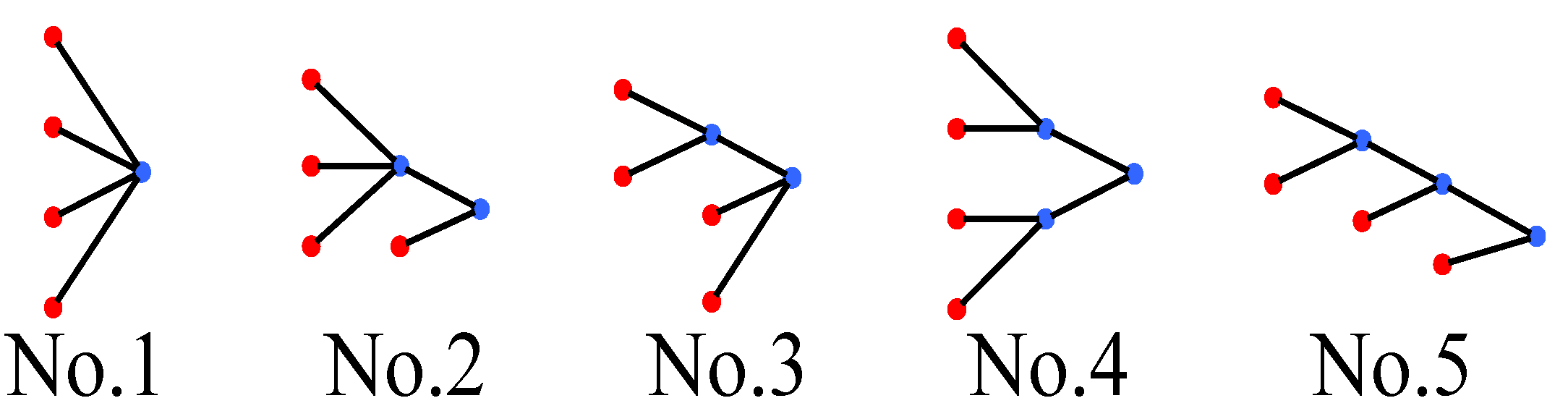
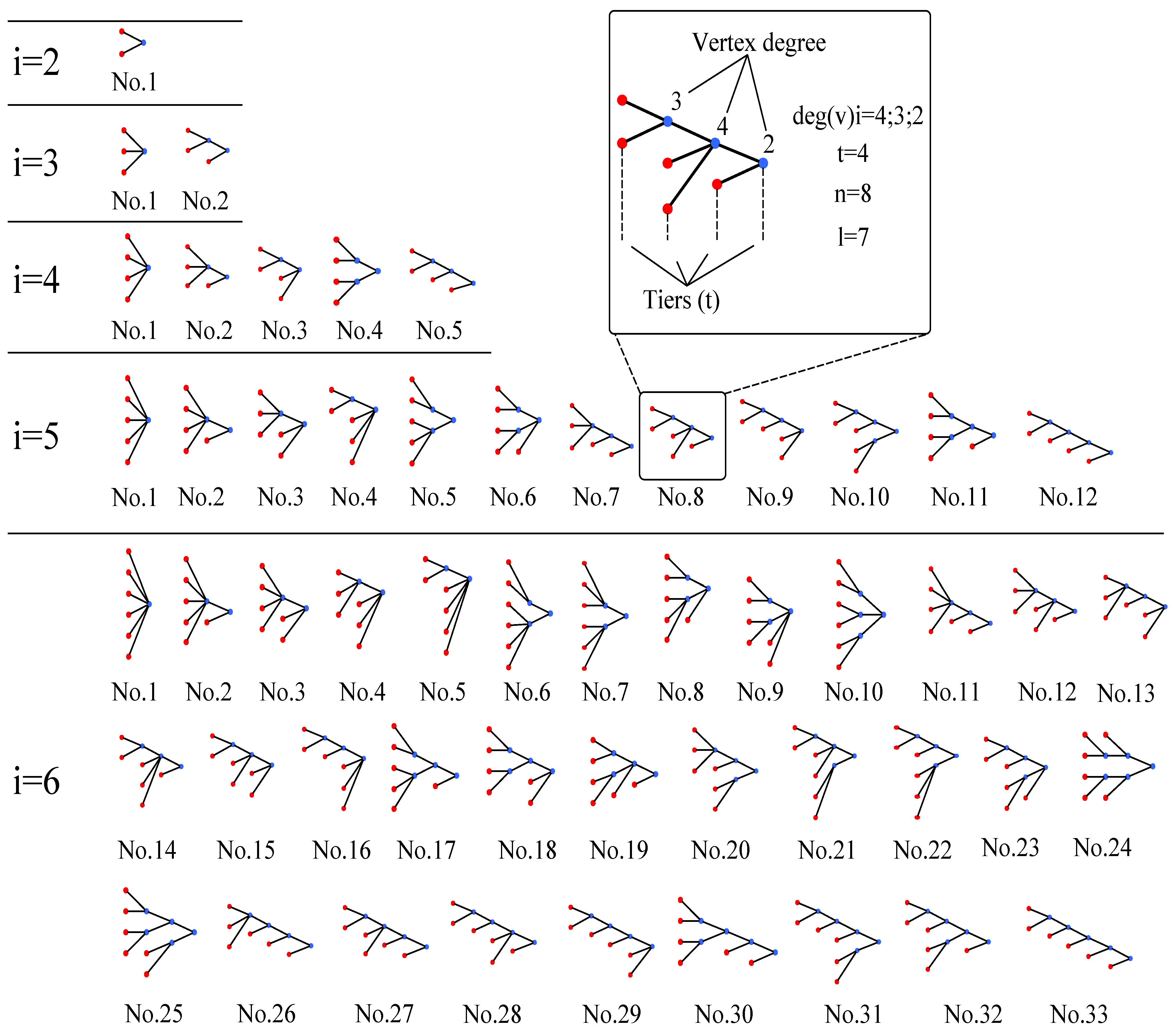
  • The initial nodes “i” in topological alternatives are allocated to possible tiers tl (l = 1,...,m), ordered from left to right, except the tier tm, in which a final assembler is situated. We assume to model ASCs only with one final assembler. In a case when a real assembly process consists of more than one final assembler (for example 3) then it is advisable, for the purpose of the complexity measuring, to split the assembly network into three independent networks.
  • The minimal number of initial nodes “i” in the first tier tl equals 2.
  • In case of non-modular assembly supply chain structure, the number of initial nodes “i” in the most upstream echelon is equal to the number of individual assembly parts or inputs (in = 1,..., r).
Then, all possible structures for given number of initial nodes “i” can be created. An example of generating the sets of structures for the classes with numbers of initial nodes from 2 to 6 is shown in Figure 2.
The numbers of all possible ASC structures for arbitrary class of a network can be determined by the following manner. We first need to calculate the sum of non-repeated combinations for each class of ASC structures through the so called the Cardinal Number [28]. The individual classes are determined by number of initial nodes “i. Then, for any integer v ≥ 2, we denote Cardinal Number by S(v) the finite set consisting of all q-tuples (v1, . . . , vq) of integers v1, . . . , vq ≥ 2 with v1 + · · · + vq ≤ v, where q is a non-negative integer.
Figure 2. Graphical models of the selected classes of ASC structures.
Entropy 15 04285 g002
The Cardinal Number #S(v) of S(v) is equal to p(v) − 1, where p(v) denotes the number of partition of “v, which increases quite rapidly with the number of initial nodes “i. For instance, for i = 2, 3, 4, 5, 6, 7, 8, 9, 10, the cardinal numbers #S(v) are given by 1, 2, 4, 6, 10, 14, 21, 29, 41 (A000065 sequence), respectively [29]. Subsequently, for each non-repeated combination “K”, a multiplication coefficient “M(K)” has to be assigned. The combination “K” is established based on the number of inputs to the final assembler “in” which is situated in tier tm (see Figure 3).
Figure 3. The transition of graphical ASC networks to the numerical combinations for i = 5.
Entropy 15 04285 g003
Then, ∑M(i)—the number for all possible combinations of ASC structures for a given class can be obtained. This number is applied in Figure 4.
Figure 4. Determination of total combinations of ASC networks related to the given classes.
Entropy 15 04285 g004
A critical step in determining all possible combinations of ASC structures for a given class (starting with a class for i = 2) are rules by which we can prescribe a multiplication coefficient “M(K)”.
In the case when we consider the number of initial nodes equals 2, there is only one numerical combination K = (1;1) corresponding with appropriate graphical model of assembly supply chain structure, and thus M(1;1) = 1. Similarly, for each non-repeated numerical combination “K” an exact logic rule has to be found. Accordingly we can formulate the following rules:
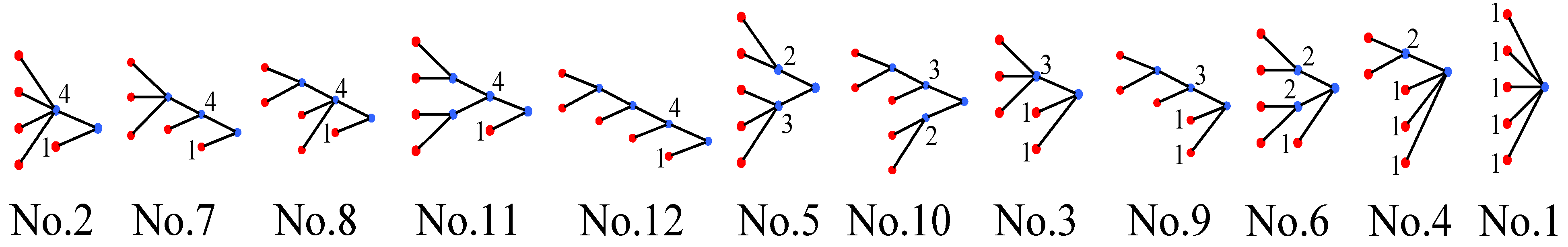
  • R1: If the numerical combination “K” consists only of numeric characters (digits), assigned by symbol “n”, n ≤ 2, e.g. K = (2;1) or K = (2;2;1) then M(2;1) or M(2;2;1) = 1.
  • R2: If the numerical combination “K” consists just of one digit “3” and other digits are < 3, e.g., K = (3;1) or (3;2;2), then M(3;1) or M(3;2;2) = 2.
  • R3: If the numerical combination “K” consists just of one digit “4” and other digits are < 3, e.g., K = (4;2), then M(4;2) = 5.
Equally, we could continue to determine multiplication coefficients “M(K)” for similar cases when numerical combinations “K” consist just of one digit ≥ 5 and other digits are < 3 or do not appear respectively. Then we would obtain the following multiplication coefficients: M(5;1) = 12; M(6;1) = 33; M(7;1) = 90; M(8;1) = 261; etc.. The multiplication coefficients for the given classes ∑M(i) in such case, follow the Sloane Integer sequence 1, 2, 5,…, 261, 766, 2312, 7068,… (A000669 sequence) [30], and are depicted in Table 1.
Table 1. Determination of all relevant alternatives for structural combinations of ASC networks.
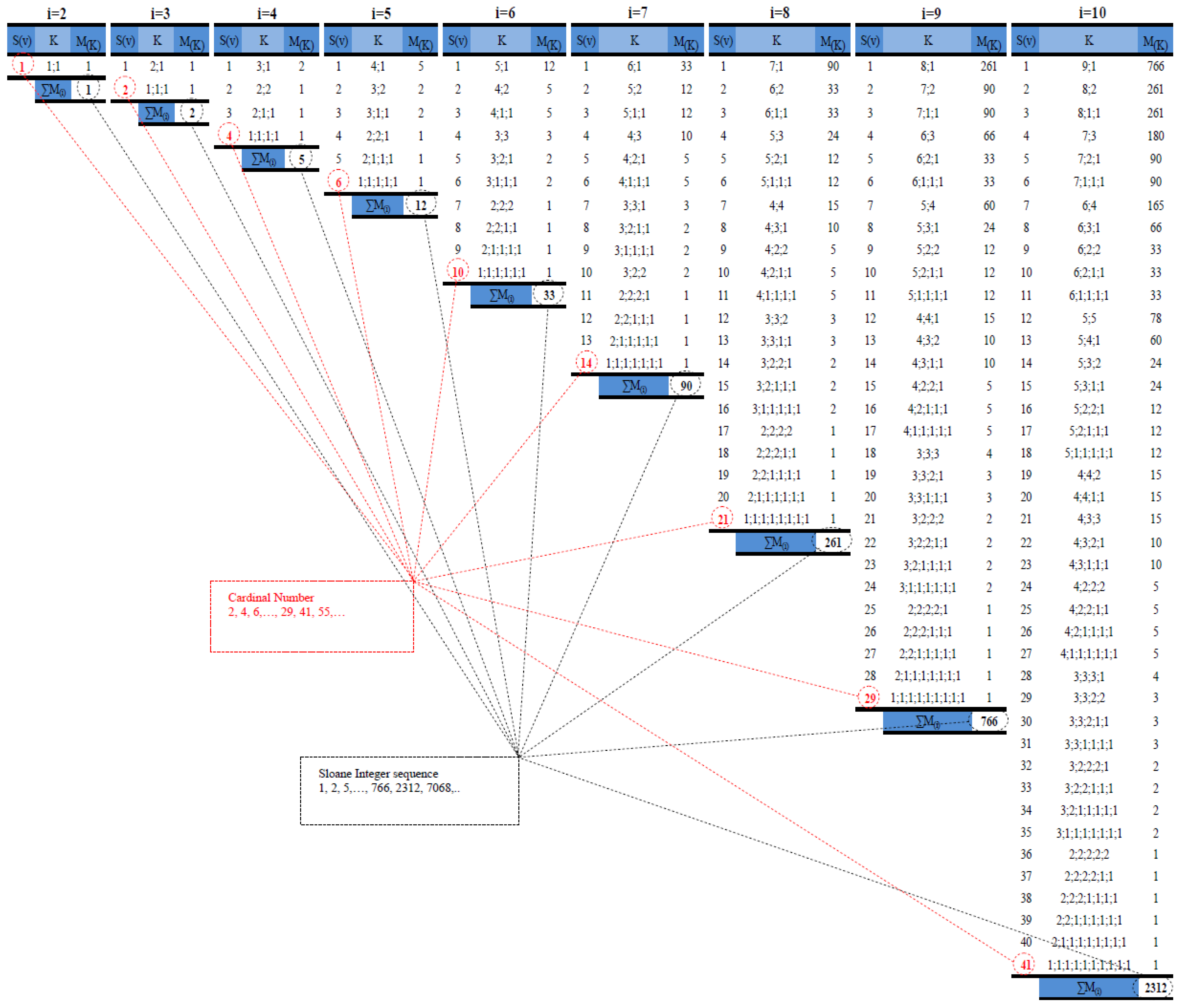
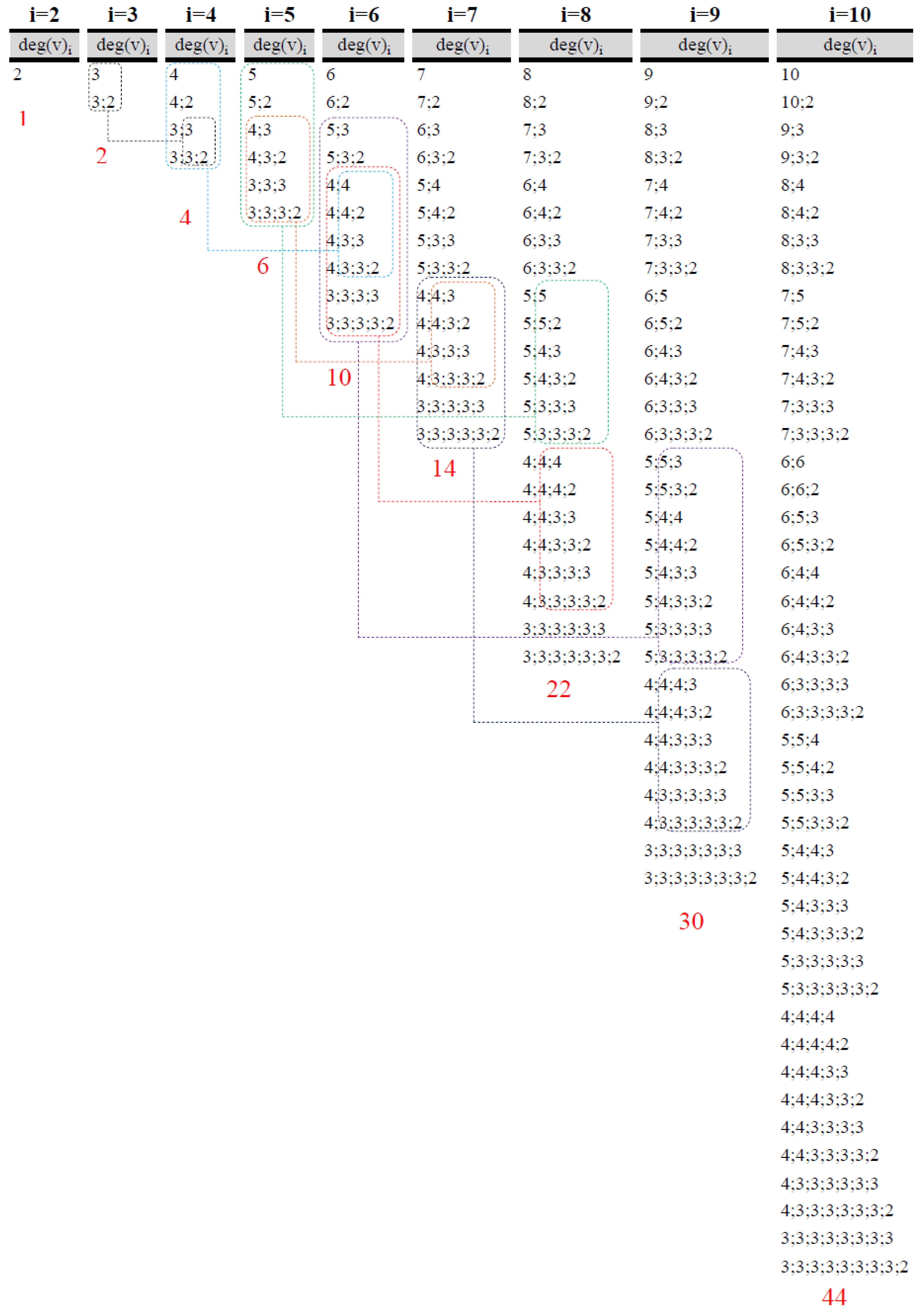
The highest digit of combination set under condition that other digits are < 3Number of alternatives for the given combinations
21
32
45
8261
9766
177,305,788
For other cases the following rules can be applied:
R4: If the numerical combination “K” consists of arbitrary number of non-repeated digits assigned as “j,k,l,…, z” that are ≥ 3 and other digits in the combination are < 3 or do not appear respectively, then the following calculation method can be used:
M ( j , k , , l , ... , z ) = M j × M k × M l × , ... , × M z
In order to apply this general rule under conditions specified in R4 the following examples can be shown:
M ( 4 ; 3 ) = M ( 4 ) × M ( 3 ) = 5 × 2 = 10
M ( 5 ; 4 ; 3 ) = M ( 5 ) × M ( 4 ) × M ( 3 ) = 12 × 5 × 2 = 120
M ( 6 ; 3 ; 2 ; 1 ) = M ( 6 ) × M ( 3 ) × M ( 2 ) × M ( 1 ) = 33 × 2 × 1 × 1 = 66
R5: If the numerical combination “K” consists just of two digits “3” and other digits in the combination are < 3 or do not appear respectively, then M(3;3) = 3. Calculation of this multiplication coefficient can be formally expressed in this manner:
M ( 3 ; 3 ) = M ( 3 ) + ( M ( 3 ) 1 ) M ( 3 , 3 ) = 2 + 1 = 3
R6: If the numerical combination “K” consists just of two digits “4” and other digits in the combination are < 3 or do not appear respectively, then M(4;4) = 15. Thus, M(4;4) is computed similarly to Equation (5):
M ( 4 ; 4 ) = M ( 4 ) + ( M ( 4 ) 1 ) + ( M ( 4 ) 2 ) + ( M ( 4 ) 3 ) + ( M ( 4 ) 4 ) M ( 4 ; 4 ) = 5 + 4 + 3 + 2 + 1 = 15
R7: If the numerical combination “K” consists just of two digits “5” and other digits in the combination are < 3 or do not appear respectively, then M(5;5) = 78 and the multiplication coefficient is computed similarly as Equations (5) and (6):
M ( 5 , 5 ) = M ( 5 ) + ( M ( 5 ) 1 ) + ( M ( 5 ) 2 ) + ( M ( 5 ) 3 ) + ( M ( 5 ) 4 ) + ( M ( 5 ) 5 ) + ( M ( 5 ) 6 ) + + ( M ( 5 ) 7 ) + ( M ( 5 ) 8 ) + ( M ( 5 ) 9 ) + ( M ( 5 ) 10 ) + ( M ( 5 ) 11 ) M ( 5 , 5 ) = 12 + 11 + 10 + 9 + 8 + 7 + 6 + 5 + 4 + 3 + 2 + 1 = 78
Analogously, we can calculate multiplication coefficients “M(K)” for arbitrary cases when numerical combinations “K” consist just of two digits n≥3 and other digits in the combination are < 3 or do not appear respectively. For such cases we can calculate the multiplication coefficients by this equation:
M ( n ; n ) = M ( n ) + ( M ( n ) 1 ) + ( M ( n ) 2 ) + , ... , + [ M ( n ) ( M ( n ) 1 ) ]
R8: If the numerical combination “K” consists just of three digits “3” and other digits in the combination are < 3 or do not appear respectively, then M(3;3;3) = 4. Calculation of this multiplication coefficient can be formally expressed in this manner:
M ( 3 ; 3 ; 3 ) = M ( 3 ; 3 ) + ( M ( 3 ; 3 ) M ( 3 ) ) + [ M ( 3 ; 3 ) M ( 3 ) ( M ( 3 ) 1 ) ] M ( 3 ; 3 ; 3 ) = 3 + ( 3 2 ) + [ 3 2 ( 2 1 ) ] = 4
R9: If the numerical combination “K” consists just of three digits “4” and other digits are < 3 or do not appear respectively, then M(4;4;4) = 15. Calculation of this multiplication coefficient can be formally expressed in this manner:
M ( 4 ; 4 ; 4 ) = M ( 4 ; 4 ) + ( M ( 4 ; 4 ) M ( 4 ) ) + + [ M ( 4 ; 4 ) M ( 4 ) ( M ( 4 ) 1 ) ] + + [ M ( 4 ; 4 ) M ( 4 ) ( M ( 4 ) 1 ) ( M ( 4 ) 2 ) ] + + [ M ( 4 ; 4 ) M ( 4 ) ( M ( 4 ) 1 ) ( M ( 4 ) 2 ) ( M ( 4 ) 3 ) ] + + [ M ( 4 ; 4 ) M ( 4 ) ( M ( 4 ) 1 ) ( M ( 4 ) 2 ) ( M ( 4 ) 3 ) ( M ( 4 ) 4 ) ] M ( 4 ; 4 ; 4 ) = 15 + ( 15 5 ) + [ 15 5 ( 5 1 ) ] + [ 15 5 ( 5 1 ) ( 5 2 ) ] + + [ 15 5 ( 5 1 ) ( 5 2 ) ( 5 3 ) ] + [ 15 5 ( 5 1 ) ( 5 2 ) ( 5 3 ) ( 5 4 ) ] = 35
R10: If the numerical combination “K” consists just of three digits “5” and other digits in the combination are < 3 or do not appear respectively, then M(5;5;5) = 78. Calculation of this multiplication coefficient can be formally expressed in this manner:
M ( 5 ; 5 ; 5 ) = M ( 5 ; 5 ) + ( M ( 5 ; 5 ) M ( 5 ) ) + + [ M ( 5 ; 5 ) M ( 5 ) ( M ( 5 ) 1 ) ] + + [ M ( 5 ; 5 ) M ( 5 ) ( M ( 5 ) 1 ) ( M ( 5 ) 2 ) ] + + [ M ( 5 ; 5 ) M ( 5 ) ( M ( 5 ) 1 ) ( M ( 5 ) 2 ) ( M ( 5 ) 3 ) ] + + [ M ( 5 ; 5 ) M ( 5 ) ( M ( 5 ) 1 ) ( M ( 5 ) 2 ) ( M ( 5 ) 3 ) ( M ( 5 ) 4 ) ] + + [ M ( 5 ; 5 ) M ( 5 ) ( M ( 5 ) 1 ) ( M ( 5 ) 2 ) ( M ( 5 ) 3 ) ( M ( 5 ) 4 ) ( M ( 5 ) 5 ) ] + + [ M ( 5 ; 5 ) M ( 5 ) ( M ( 5 ) 1 ) ( M ( 5 ) 2 ) ( M ( 5 ) 3 ) ( M ( 5 ) 4 ) ( M ( 5 ) 5 ) ( M ( 5 ) 6 ) ] + + [ M ( 5 ; 5 ) M ( 5 ) ( M ( 5 ) 1 ) ( M ( 5 ) 2 ) ( M ( 5 ) 3 ) ( M ( 5 ) 4 ) ( M ( 5 ) 5 ) ( M ( 5 ) 6 ) , ... , ( M ( 5 ) 11 ) ] M ( 5 ; 5 ; 5 ) = 78 + 66 + 55 + 45 + 36 + 28 + 21 + 15 + 10 + 6 + 3 + 1 = 364
A general rule to calculate the multiplication coefficients “M(K)” for arbitrary cases (when numerical combinations “K” consist just of three digits n ≥ 3 and other digits in the combination are < 3 or do not appear respectively) can be derived using the previous rules R8, R9 and R10 a formally can be expressed as:
M ( n ; n ; n ) = M ( n ; n ) + ( M ( n ; n ) M ( n ) ) + + [ M ( n ; n ) M ( n ) ( M ( n ) 1 ) ] + + [ M ( n ; n ) M ( n ) ( M ( n ) 1 ) ( M ( n ) 2 ) ] + , ... , + + { M ( n ; n ) M ( n ) ( M ( n ) 1 ) ( M ( n ) 2 ) , ... , [ M ( n ) ( M ( n ) 1 ) ] }
Obviously, there are other specific cases of numerical combinations for which multiplication coefficients can be formulated in exact terms.

4. Static Structural Complexity Metrics for ASC Structures

4.1. Some Terminology and Definitions

The following section consists of theoretical concepts and working definitions for the given research domain. General networks can be properly defined as well as effectively recognized as structural patterns by graph theory (GT). GT deals with the mathematical properties of structures as well as with problems of a general nature. In this context, a graph is a network of nodes (vertices) and links (edges) from some nodes to others or to themselves. Graph G consists of a set of V vertices, {V}≡{v1, v2, … , vV}, and the set of E edges, {E}≡{e1, e2, … , eE}. The edge {e1} is the path from vertex v1 and ends in vertex vV. The number of the nearest-neighbors of a vertex v1 is termed vertex degree and denoted deg(v). The maximum degree of a graph G, denoted by Δ(G), and the minimum degree of a graph, denoted by δ(G), are the maximum and minimum degree of its vertices. For a vertex, the number of head endpoints adjacent to a vertex is called the in-degree of the vertex and the number of tail endpoints is its out-degree. For a directed graph, the sum of the vertex in-degree and out-degree is the vertex degree [31].
deg ( v ) = deg + ( v ) i + deg ( v ) i

4.2. Specifications of ASC Networks Complexity Measure

According to Shannon’s information theory, the entropy of information H(α) in describing a message of N system elements (or symbols), distributed according to some equivalence criterion α into k groups of N1, N2,…, Nk elements, is calculated by the formula:
H ( α ) = i = 1 k p i log 2 p i = i = 1 k N i N log 2 N i N ,
where pi specifies the probability of occurrence of the elements of the ith group.
Since it is of interest to characterize entropy of information of a network according to (14), we can to substitute symbols or system elements for the vertices. In order to define the probability for a randomly chosen system element “i” it is possible to formulate general weight function as pi = wi / Σwi, assuming that Σpi = 1. Considering the system elements, the vertices, and supposing the weights assigned to each vertex to be the corresponding vertex degrees, one easily distinguishes the null complexity of the totally disconnected graph from the high complexity of the complete graph [32]. Then, the probability for a randomly chosen vertex i in the complete graph of V vertices to have a certain degree deg(v)i can be expressed by formula:
p i = deg ( v ) i i = 1 V deg ( v ) i
Shannon defines information as:
I = H max H ,
where Hmax is maximum entropy that can exist in a system with the same number of elements.
Subsequently, the information entropy of a graph with a total weight W and vertex weights wi can be expressed in the form of the equation:
H ( W ) = W log 2 W i = 1 V w i log 2 w i
Since the maximum entropy is when all wi = 1, then
H max = W log 2 W
By substituting W = deg(v)i and wi = deg(v)i, the information content of the vertex degree distribution of a network called as Vertex degree index (Ivd) is derived by Bonchev and Buck [32] that is expressed as follows:
I v d = i = 1 V deg ( v ) i log 2 deg ( v ) i
Based on our previous comparison [33,34] of Vertex degree index with another complexity measures we can confirm that Ivd meet given criteria for a complexity assessment of networks in the best way. For the evaluation of complexity indicators the correlation based on Spearman's rank correlation coefficient between different methods of complexity measures was used.
Figure 5. The graphical principle of generating non-repeated structures based on vertex degree parameter.
Entropy 15 04285 g005

4.3. Selection of ASC Networks with Non-repeated Sets of Vertex Degrees

For the next step it is useful to assign values of vertex degrees to each node of the networks excluding a case when the value = 1 (as it can be seen in Figure 2). However, we have to take into consideration the existence of graphs of the same class with a repeated set of vertex degrees. In order to omit such superfluous structures it is purposeful to select from the classes of ASC structures only the graphs with a non-repeated set of vertex degrees and to order them in systematic way. Then we obtain the exact sums of such graphs, as it shown in Figure 5. For instance, when number of initial nodes i = 6, then sum of graphs equals 10. Figure 5 also provides graphical principle of generating non-repeated structures.
When applying the Vertex degree index to assess the configuration complexity of clustered ASC networks with the non-repeated set of vertex degrees we gain values of complexity depicted in Figure 6. Then, we can compare complexity of optional assembly supply chain networks. From this figure we can see that complexity values of ASC structures for ascending ordered classes grow smaller and smaller.
Figure 6. Computational results of the Ivd for selected classes “i” of ASC structures.
Entropy 15 04285 g006

5. The Concept of Quantitative Complexity Scale for ASC Networks

Basically, the comparison of complexity is of a relative and subjective nature. It is also clear that through a relative complexity metric we can compare the complexity of the existing configuration against the simplest or/and the most complex one from the same class of ASC network. Perhaps, the most important feature of the relative complexity metric is that we can generalize it to other areas [35]. Accordingly, when we apply this complexity measure for the complete graphs with v(v−1)/2 edges we can get upper bounds for configuration complexity of any ASC structure with a given number of vertices. Obtained upper bounds derived from complexity values of selected complete graphs are shown in Figure 7.
Figure 7. Graph of the complexity measures for the selected complete graphs.
Entropy 15 04285 g007
When considering the fact that obtained complexity values for the complete graphs grow larger and larger, while complexity values of ASC structures for ascending ordered classes grow smaller and smaller it gives a realistic chance to establish quantitative complexity degrees of ASC networks. Under this assumption, arbitrary ASC networks can be categorize into quantitative configuration complexity degrees that are shown in Figure 8. In such case, the actual question arises regarding how many degrees of structural complexity are really needed to comprise all ASCs that we know exists. The seven-degree scale of structural complexity is based on inductive reasoning. For example, upper bound for configuration complexity of ASC networks with i = 10 equals 40.04. Indeed, it is very presumable that practically all realistic ASC networks wouldn’t reach higher structural complexity than 216 what presents structural complexity for K9. However, in this context, it is necessary to take under consideration a relation between complexity and usability [36]. In this case it would be needed to estimate an optimal degree of structural complexity under when the usability of ASC networks is critical for its success.
Figure 8. Proposed quantitative complexity degrees.
Entropy 15 04285 g008

6. Conclusions

The main contributions of this paper consist of the following four aspects:
(1)
A new exact framework for creating topological classes of ASC networks is developed. This methodological framework enables one to determine all relevant topological graphs for any class of ASC structure. The usefulness of such a framework is especially notable in cases when it is necessary to apply relative complexity metrics to compare the complexity of the existing configuration against the simplest or/and the most complex one.
(2)
In order to parameterize properties of vertices of the ASC networks, an efficient method to identify total number of the graphs with non-repeated sets of vertex degrees structure is presented. The determination of the non-repeated sets of vertex degrees structure (for selected classes of ASC networks are described in Figure 5) shows that the total numbers of such graphs follows the Omar integer sequence [37], with the first number omitted.
(3)
The Vertex degree index was applied to a new area of configuration complexity.
(4)
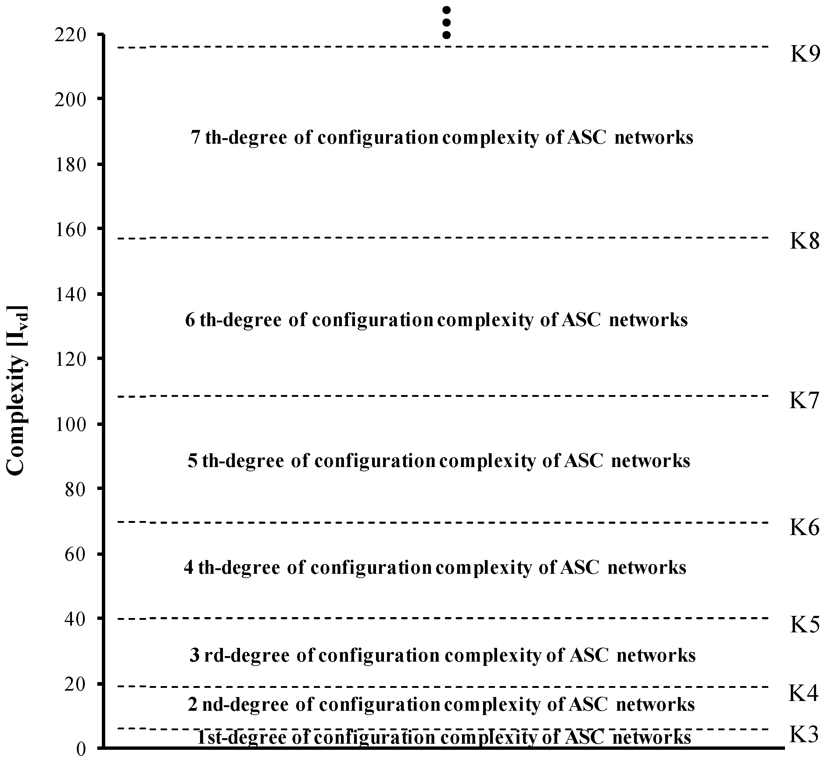
The quantitative object-oriented model for defining degrees of configuration complexity of ASC networks was outlined.
The proposed approach to relative complexity assessment may easily be applied at the initial design stages as well as in decision-making process along with other important considerations such as operational complexity issues. However, this research path requires further independent research to confirm this preliminary results and proposals.

Acknowledgments

This work has been supported by the financing from KEGA grant - Cultural and Education Grant Agency of Ministry of School, Science, Research and Sport of Slovak Republic.

Conflicts of Interest

The authors declare no conflict of interest.

References

  1. Hartmanis, J. New developments in structural complexity theory. Theor. Comput. Sci. 1990, 71, 79–93. [Google Scholar] [CrossRef]
  2. Manson, S.M. Simplifying complexity: a review of complexity theory. Geoforum 2001, 32, 405–414. [Google Scholar] [CrossRef]
  3. ElMaraghy, W.; ElMaraghy, H.; Tomiyama, T.; Monostori, L. Complexity in engineering design and manufacturing. CIRP Ann. Manuf. Technol. 2012, 61, 793–814. [Google Scholar] [CrossRef]
  4. Kolmogorov, A.N. Three Approaches to the Quantitative definition of information. Probl. Inf. Transm. 1965, 1, 1–7. [Google Scholar] [CrossRef]
  5. Chaitin, G. On the Length of programs for computing finite binary sequences. J. ACM. 1966, 13, 547–569. [Google Scholar] [CrossRef]
  6. Shannon, C.E. A mathematical theory of communication. Bell Syst. Technol. J. 1948, 27, 379–423. [Google Scholar] [CrossRef]
  7. Bonchev, D.; Trinajstic, N. Information theory, distance matrix and molecular branching. J. Chem. Phys. 1977, 67, 4517–4533. [Google Scholar] [CrossRef]
  8. Bonchev, D.; Kamenska, V. Information theory in describing the electrionic structure of atoms. Croat. Chem. Acta 1978, 51, 19–27. [Google Scholar]
  9. Bochnev, D. Information indices for atoms and molecules. MATCH-Commun. Math. Co. 1979, 7, 65–113. [Google Scholar]
  10. Grassberger, P. Information and complexity measures in dynamical systems. In Information Dynamics; Atmanspacher, H., Scheingraber, H., Eds.; Plenum Press: New York, NY, USA, 1991; Volume 1, pp. 15–33. [Google Scholar]
  11. Crutchfield, J.P.; Young, K. Inferring statistical complexity. Phys. Rev. Lett. 1989, 63, 105–108. [Google Scholar] [CrossRef] [PubMed]
  12. Bucki, R.; Chramcov, B. Information support for logistics of manufacturing tasks. Int. J. Math. Mod. Meth. App. Sci. 2013, 7, 193–203. [Google Scholar]
  13. Ouchi, W.G. The relationship between organizational structure and organizational control. Admin. Sci. Q. 1977, 22, 95–113. [Google Scholar] [CrossRef]
  14. Blau, P.M.; Schoenherr, R.A. The Structure of Organizations; Basic Books: New York, NY, USA, 1971; pp. 1–445. [Google Scholar]
  15. Blau, P.M.; Scott, W.R. Formal Organizations; Chandler Publishing Co.: San Francisco, CA, USA, 1962; pp. 1–312. [Google Scholar]
  16. Strogatz, S.H. Exploring complex networks. Nature 2001, 410, 268–276. [Google Scholar] [CrossRef] [PubMed]
  17. Blecker, T.; Kersten, W.; Meyer, C. Development of an approach for analyzing supply chain complexity. In Mass Customization. Concepts – Tools – Realization; Blecker, T., Friedrich, G., Eds.; Gito Verlag: Klagenfurt, Austria, 2005; Volume 1, pp. 47–59. [Google Scholar]
  18. Frizelle, G.; Suhov, Y.M. An entropic measurement of queueing behaviour in a class of manufacturing operations. Proc. Royal Soc. London Series. 2001, 457, 1579–1601. [Google Scholar] [CrossRef]
  19. AlGeddawy, T.; Samy, S.N.; Espinoza, V. A model for assessing the layout structural complexity of manufacturing systems. J. Manuf. Sys. in press.
  20. Hasan, M.A.; Sarkis, J.; Shankar, R. Agility and production flow layouts: An analytical decision analysis. Comput. Ind. Eng. 2012, 62, 898–907. [Google Scholar] [CrossRef]
  21. MacDuffie, J.P.; Sethurman, K.; Fisher, M.L. Product variety and manufacturing performance: Evidence from the international automotive assembly plant study. Manag. Sci. 1996, 42, 350–369. [Google Scholar] [CrossRef]
  22. Schleich, H.; Schaffer, L.; Scavarda, F. Managing complexity in automotive production. In Proceedings of the 19th international conference on production research, Valparaiso, Chile, 29 July–2 August 2007.
  23. Fast-Berglund, A.; Fässberg, T.; Hellman, F.; Davidsson, A.; Stahrea, J. Relations between complexity, quality and cognitive automation in mixed-model assembly. J. Manuf. Sys. 2013, 32, 449–455. [Google Scholar]
  24. Zou, Z.H.; Morse, E.P. Statistical tolerance analysis using GapSpace. In Proceedings of the 7th CIRP Seminar, Cachan, France, 24–25 April 2001.
  25. Zhu, X.; Hu, S.J.; Koren, Y.; Huang, N. A complexity model for sequence planning in mixed-model assembly lines. J. Manuf. Sys. 2012, 31, 121–130. [Google Scholar] [CrossRef]
  26. Samy, S.N. Complexity of products and their assembly systems. Ph.D. Thesis, University of Windsor, Ontario, Canada, June 2011. [Google Scholar]
  27. Hu, S.J.; Zhu, X.W.; Wang, H.; Koren, Y. Product variety and manufacturing complexity in assembly systems and supply chains. CIRP Ann. Manuf. Technol. 2008, 57, 45–48. [Google Scholar] [CrossRef]
  28. Deiser, O. On the development of the notion of a cardinal number. Hist. Philos. Logic 2010, 2, 123–143. [Google Scholar] [CrossRef]
  29. Sloane, N.J.A.; Plouffe, S. The Encyclopedia of Integer Sequences; Academic Press: San Diego, CA, USA, 1995; pp. 1–587. [Google Scholar]
  30. Sloane, N.A.J. A Handbook of Integer Sequences; Academic Press: Boston, MA, USA, 1973; pp. 1–206. [Google Scholar]
  31. Barrat, A.; Barthelemy, M.; Vespignani, A. Dynamical Processes on Complex Networks; Cambridge University Press: Cambridge, UK, 2008; pp. 1–368. [Google Scholar]
  32. Bonchev, D.; Buck, G.A. Quantitative measures of network complexity. In Complexity in Chemistry, Biology and Ecology; Bonchev, D., Rouvray, D.H., Eds.; Springer: New York, NY, USA, 2005; pp. 191–235. [Google Scholar]
  33. Modrak, V.; Marton, D. Complexity metrics for assembly supply chains: A comparative study. Adv. Mat. Res. 2013, 629, 757–762. [Google Scholar] [CrossRef]
  34. Modrak, V.; Marton, D.; Kulpa, W.; Hricova, R. Unraveling complexity in assembly supply chain networks. In Proceedings of the LINDI 2012—4th IEEE International Symposium on Logistics and Industrial Informatics, Smolenice, Slovakia, 5–7 September 2012; pp. 151–156.
  35. Munson, J.C.; Khoshgoftaar, T.M. Applications of a relative complexity metric for software project management. J. Syst. Soft. 1990, 12, 283–291. [Google Scholar] [CrossRef]
  36. Comber, T.; Maltby, J. Investigating layout complexity. In Computer-Aided Design of User Interfaces; Vanderdonckt, J., Ed.; Press Universitaires de Namur: Namur, country, 1996; pp. 209–227. [Google Scholar]
  37. The on-line encyclopedia of integer sequences (OEIS). http://oeis.org/A139582 (accessed on 6 February 2013).

