Analogue Realization of Fractional-Order Dynamical Systems


 and
and 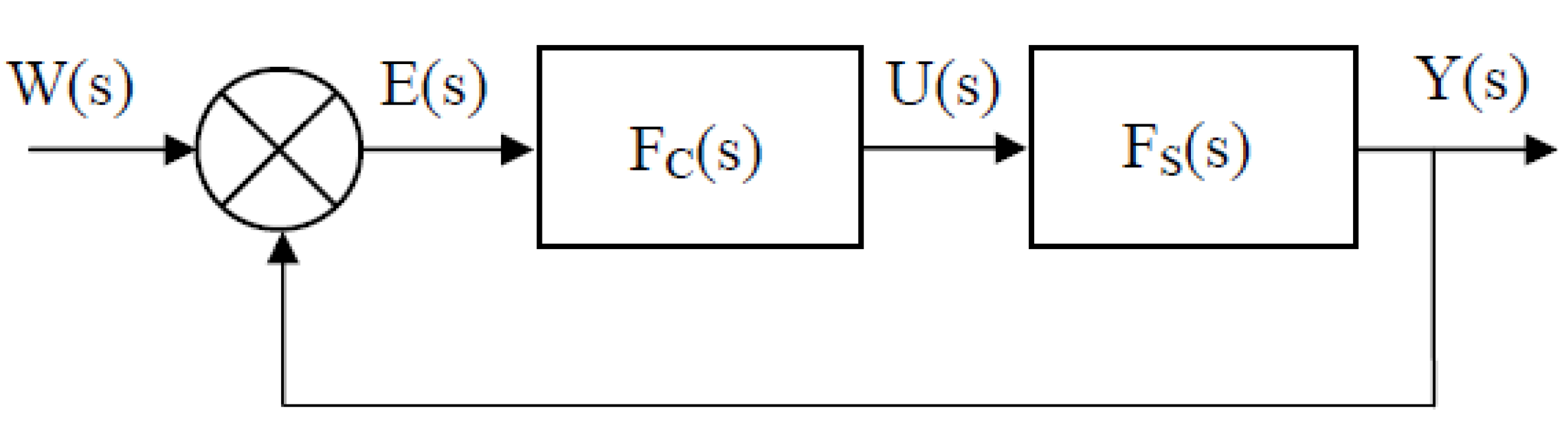
Abstract
:1. Introduction
2. Definition of the Fractional Order Control System and Its Model

2.1. Fractional-Order Differential Equation
2.2. Fractional-Order Laplace Transfer Function
3. Principles of Electronic Realization of the FO Dynamical System
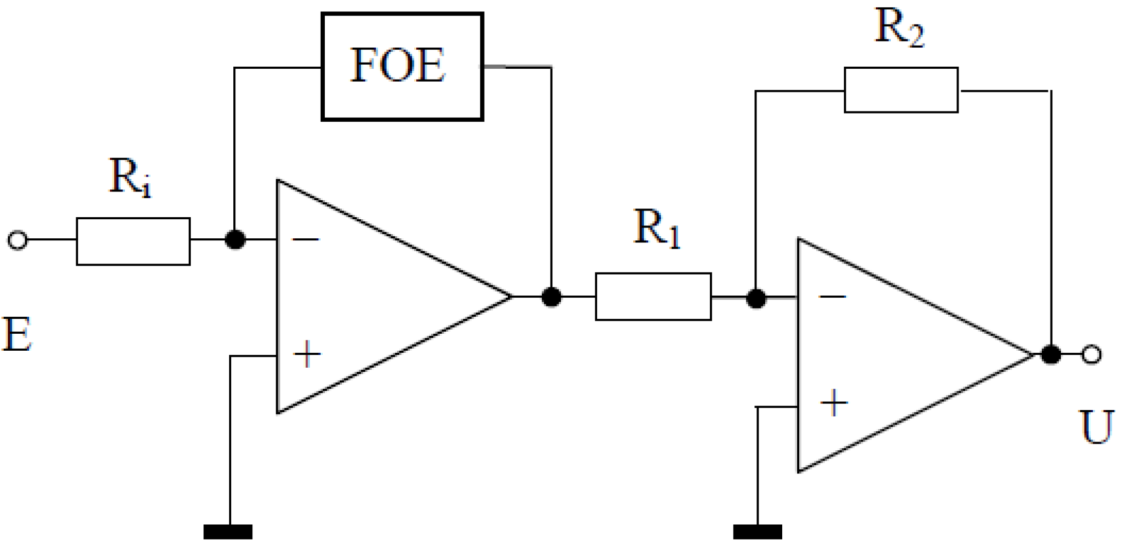
3.1. Principles of Electronic Realization of the FO Integrator and Differentiator

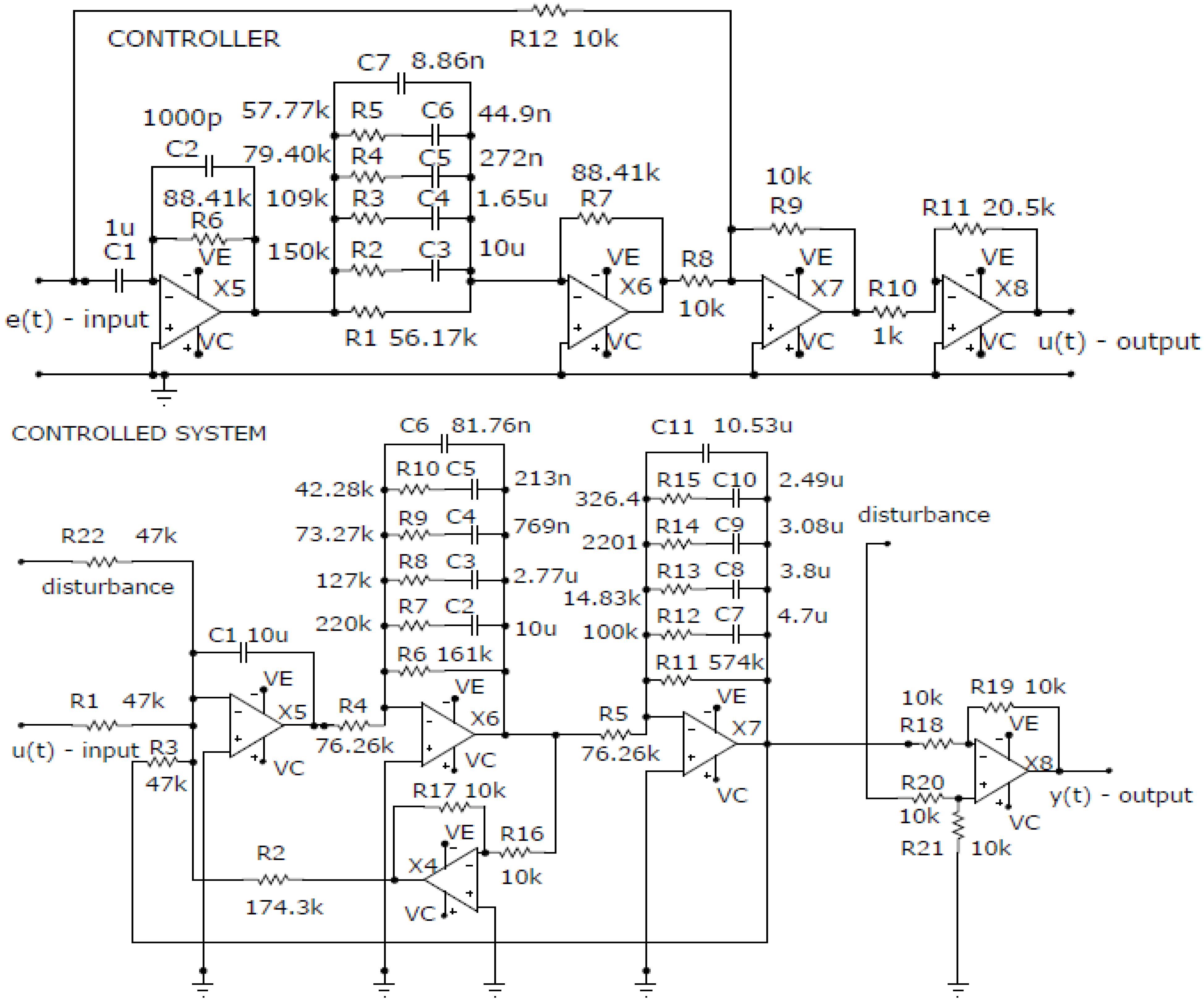
3.2. Principles of Electronic Realization of the FO Controlled System and Controller


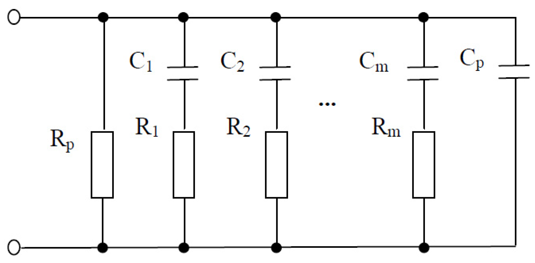
3.3. Design Procedure of the Fractional-Order Element

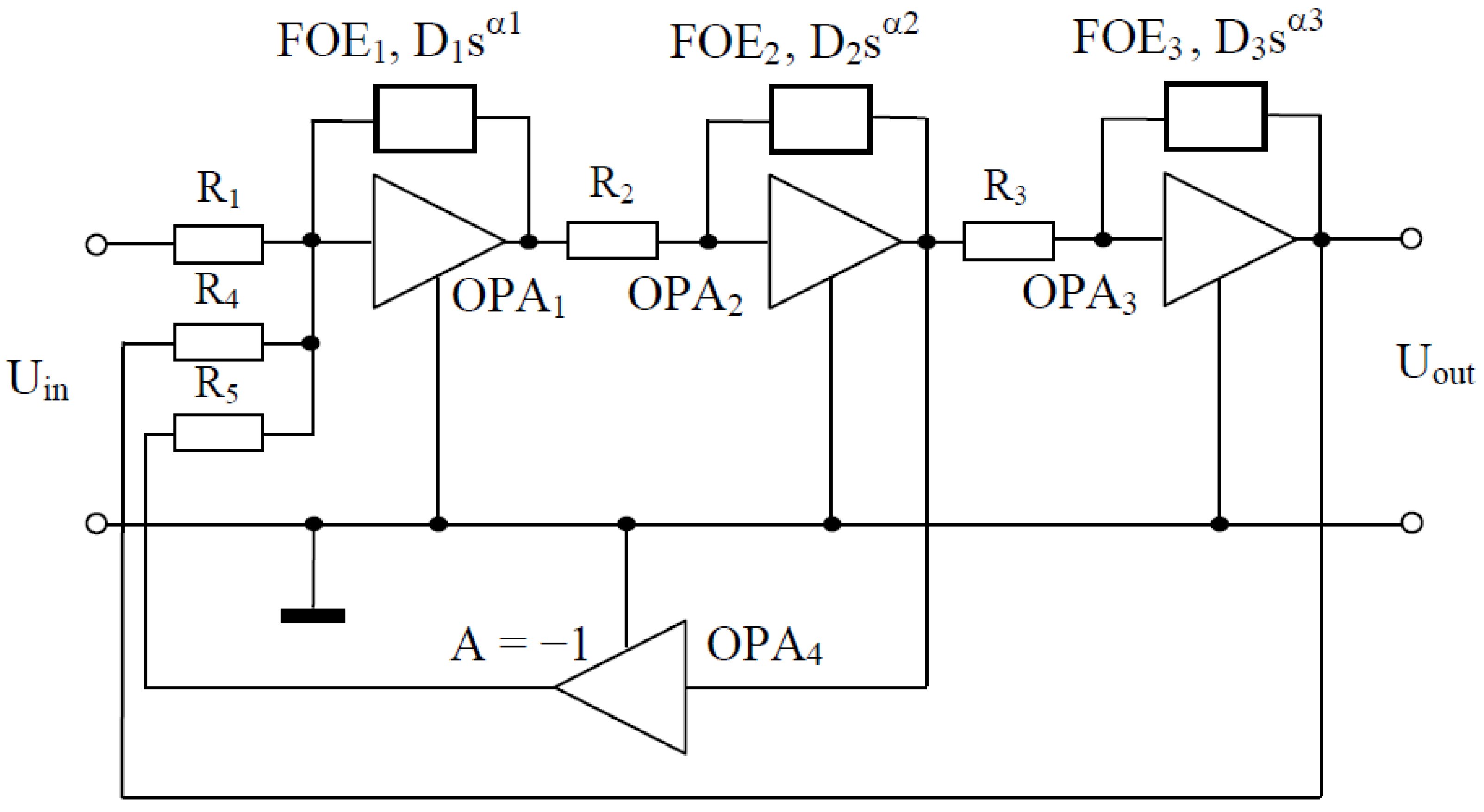
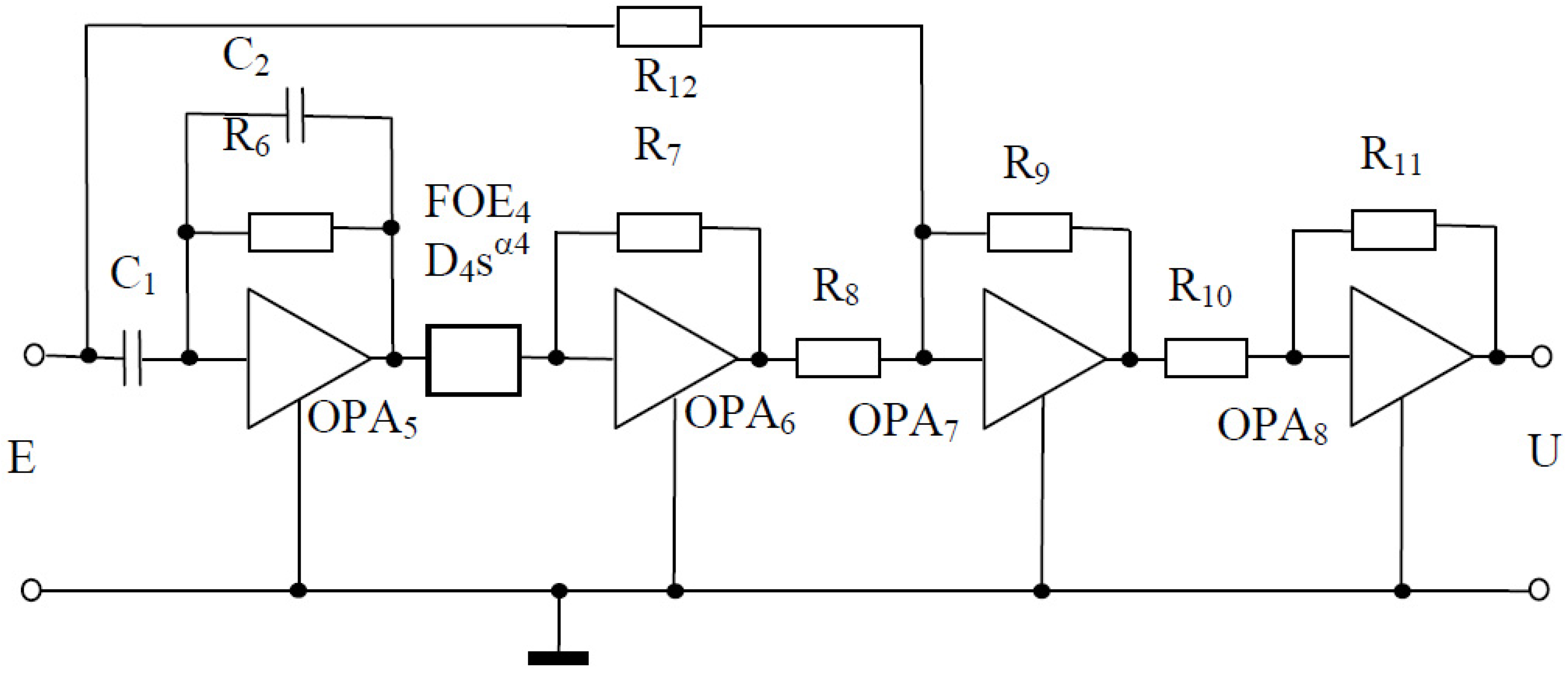
4. Design of the FOE for the Considered Control System
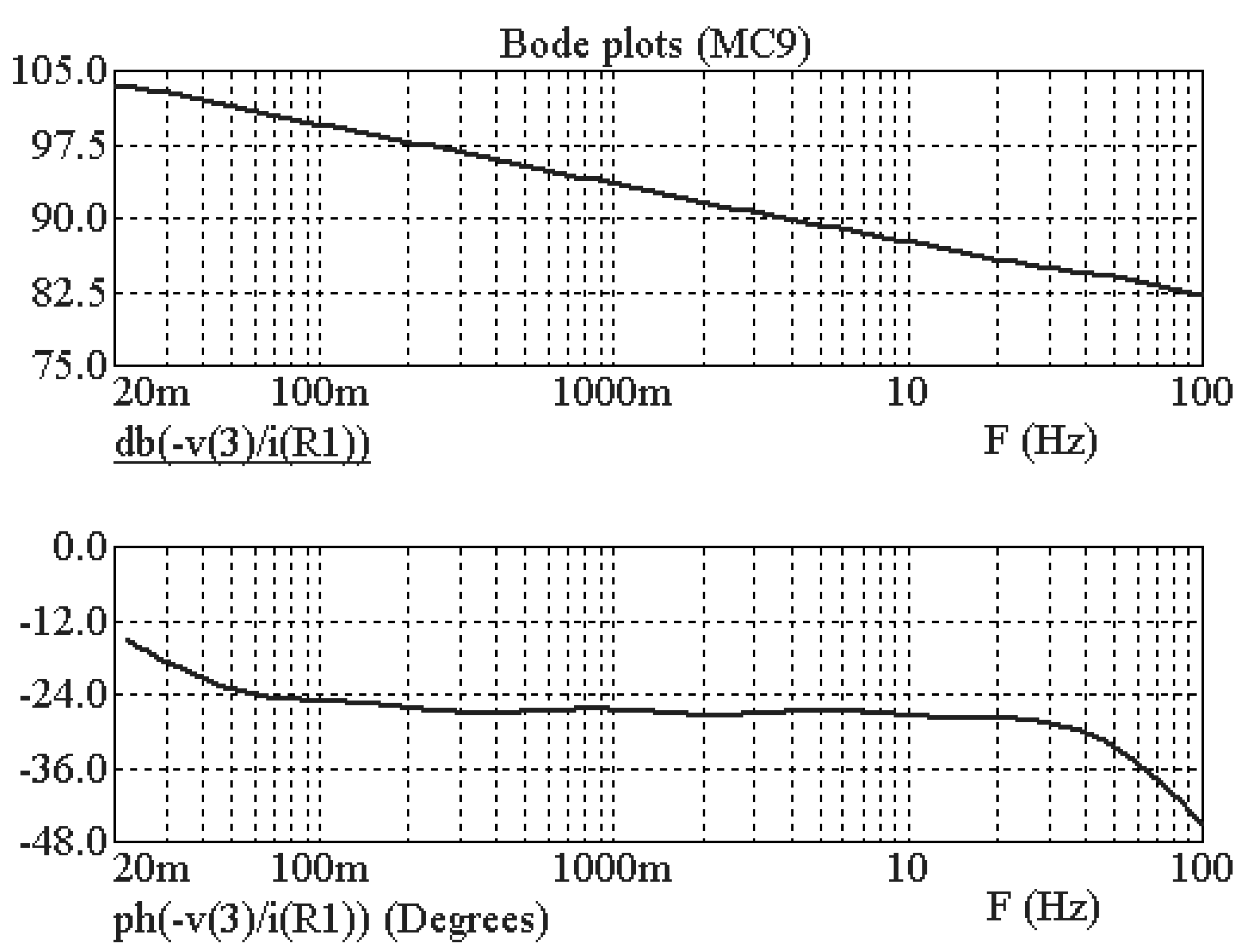

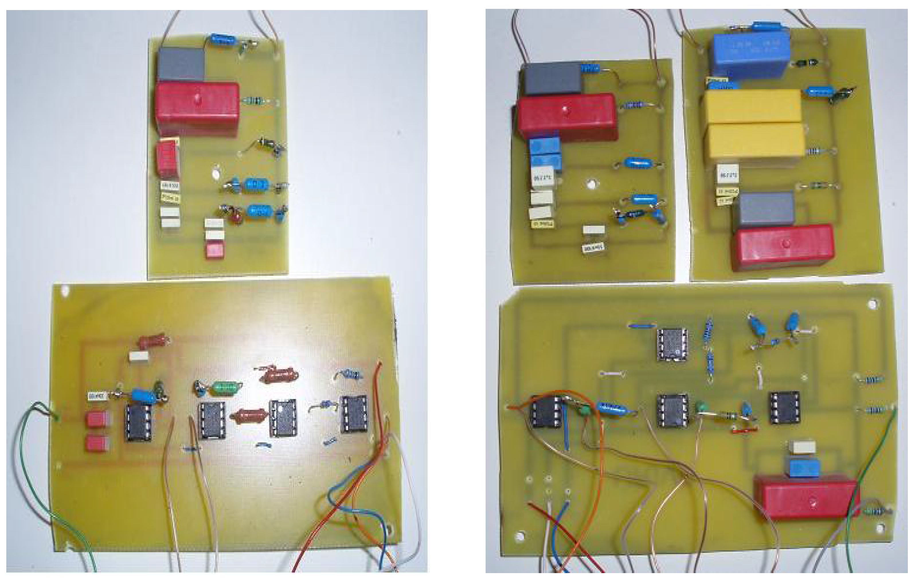
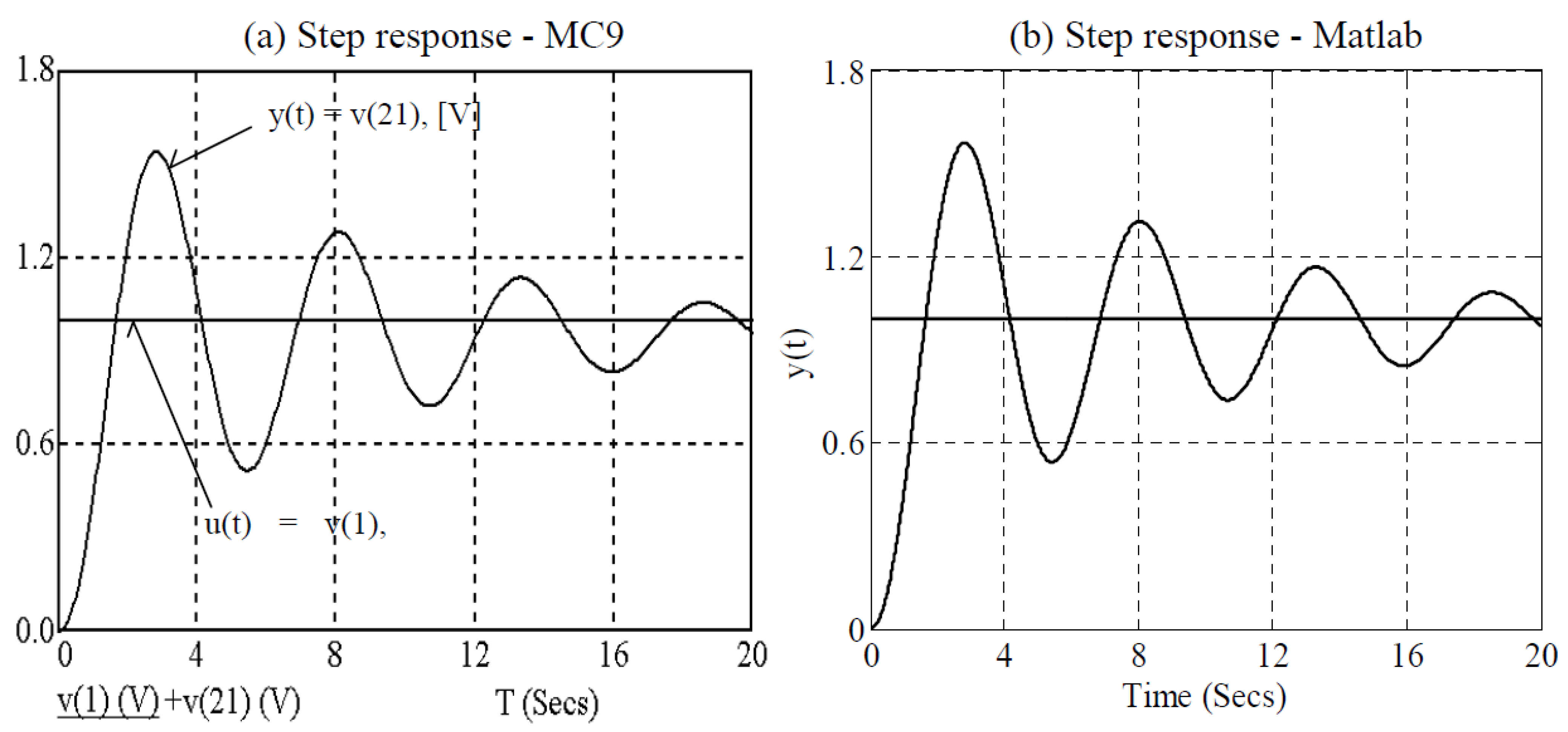
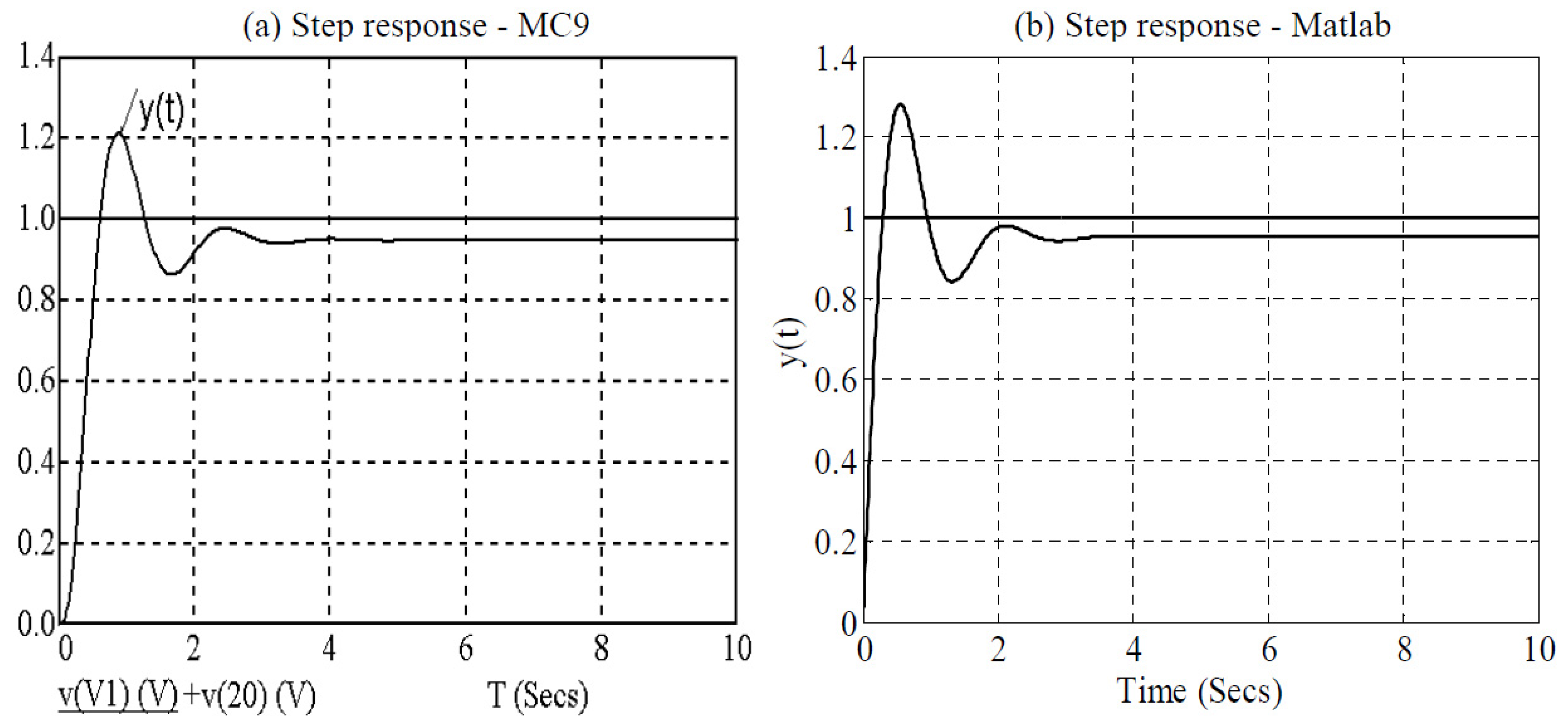
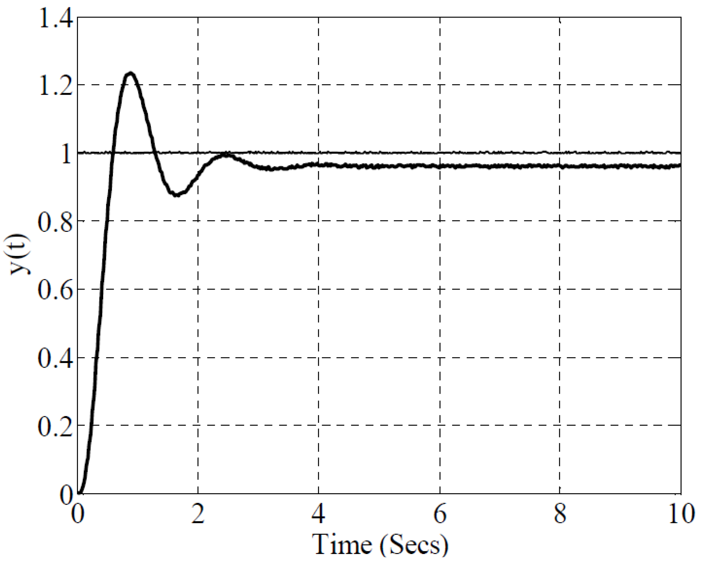
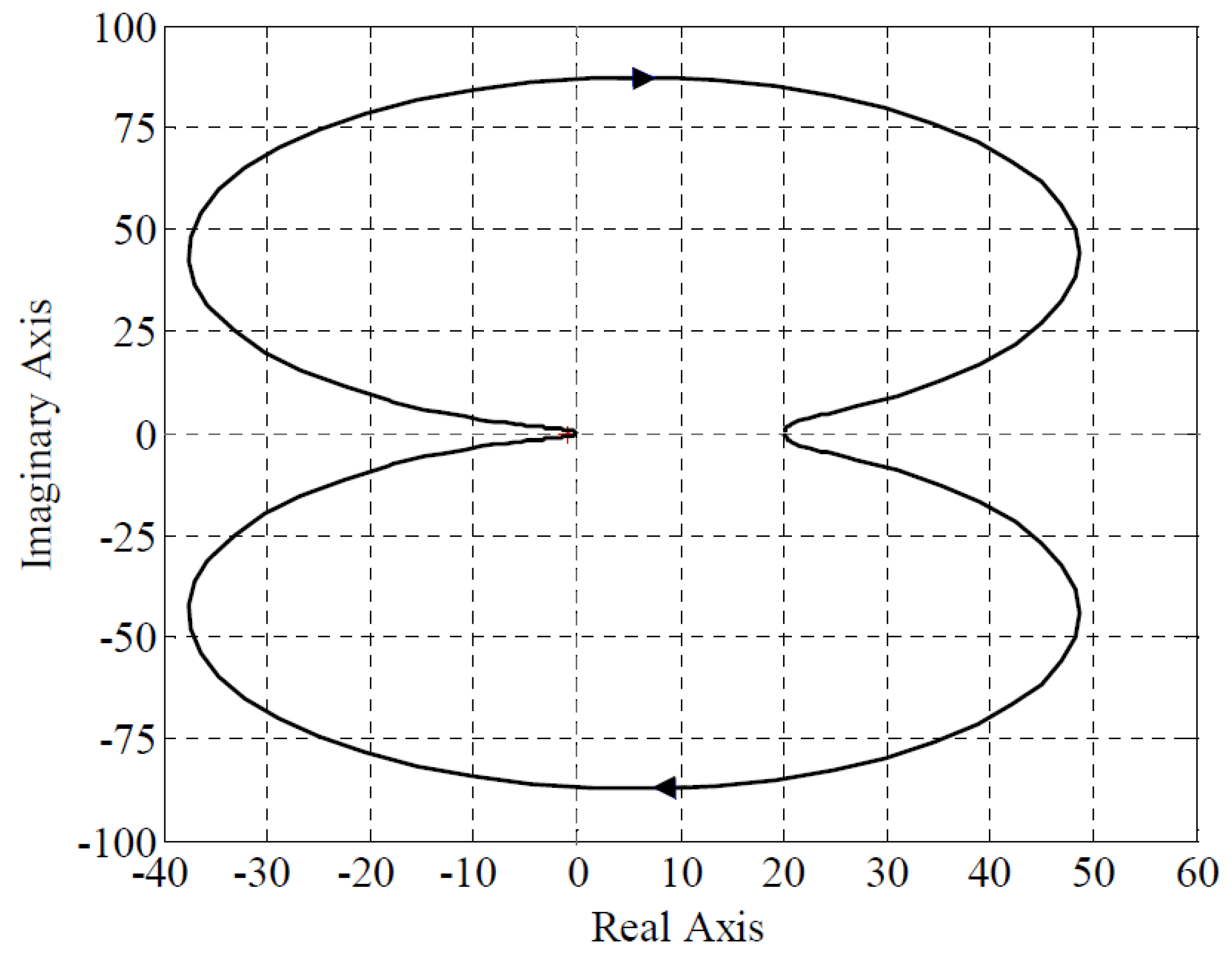
5. Verification of the Analogue Realization of the FO Control System


6. Conclusions
Acknowledgments
Conflicts of Interest
References
- Manabe, S. The Non-Integer Integral and its Application to Control Systems. ETJ Japan 1961, 6, 83–87. [Google Scholar]
- Outstaloup, A. From fractality to non integer derivation through recursivity, a property common to these two concepts: A fundamental idea from a new process control strategy. In Proceedings of the 12th IMACS World Congress, Paris, France, 18–22 July 1988; pp. 203–208.
- Oldham, K.B.; Spanier, J. The Fractional Calculus; Academic Press: New York, NY, USA, 1974. [Google Scholar]
- Axtell, M.; Bise, M.E. Fractional Calculus Applications in Control Systems. In Proceedings of the IEEE 1990 National Aerospace and Electronics Conference, New York, NY, USA, 21–25 May 1990; pp. 563–566.
- Kalojanov, G.D.; Dimitrova, Z.M. Teoretiko-experimentalnoe opredelenie oblastej primenimosti sistemy PI (I) reguliator-objekt s necelocislennoj astaticnostiu, (Theoretico-experimental determination of the domain of applicability of the system PI (I) regulator—fractional-type astatic systems). Izvestia vyssich ucebnych zavedenij, Elektromechanika 1992, 2, 65–72. (in Russian). [Google Scholar]
- Samko, S.G.; Kilbas, A.A.; Marichev, O.I. Fractional Integrals and Derivatives: Theory and Applications; Gordon and Breach Science Publishers: Yverdon, Switzerland, 1993. [Google Scholar]
- Miller, K.S.; Ross, B. An Introduction to the Fractional Calculus and Fractional Differential Equations; Wiley: New York, NY, USA, 1993. [Google Scholar]
- Podlubny, I. The Laplace transform method for linear differential equations of the fractional order. In UEF-02-94; The Academy of Science Institute of Experimental Physics: Košice, Slovak Republic, 1994; Available online: http://arxiv.org/abs/funct-an/9710005 (accessed on 30 October 1997).
- Podlubny, I. Fractional Differential Equations; Academic Press: San Diego, CA, USA, 1999. [Google Scholar]
- Podlubny, I.; Dorcak, L.; Misanek, J. Application of fractional-order derivates to calculation of heat load intensity change in blast furnace walls. Trans. TU Kosice 1995, 5, 137–144. [Google Scholar]
- Dorcak, L.; Terpak, J.; Podlubny, I.; Pivka, L. Methods for monitoring of heat flow intensity in the blast furnace wall. Metalurgija 2010, 49, 75–78. [Google Scholar]
- Gabano, J.D.; Poinot, T.; Kanoun, H. Identification of a thermal system using continuous linear parameter-varying fractional modeling. Control Theory Appl. 2011, 5, 889–899. [Google Scholar] [CrossRef]
- Victor, S.; Melchior, P.; Nelson-Gruel, D.; Oustaloup, A. flatness control for linear fractional MIMO systems: Thermal application. In Proceedings of the 3rd IFAC Workshop on Fractional Differentiation and Its Application, Ankara, Turkey, 5–7 November 2008; pp. 5–7.
- Barbosa, R.S.; Machado, J.A.T.; Silva, M.F. Time domain design of fractional differ integrators using least-squares. Signal Process. 2006, 86, 2567–2581. [Google Scholar] [CrossRef]
- Ortigueira, M.D.; Machado, J.A.T. Fractional signal processing and applications. Signal Process. 2003, 83, 2285–2286. [Google Scholar] [CrossRef]
- Bar-Yam, Y. Dynamics of Complex Systems; Perseus Books Reading: Cambridge, MA, USA, 1997. [Google Scholar]
- Zhou, S.; Chen, Y.Q. Genetic Algorithm-based identification of fractional-order systems. Entropy 2013, 15, 1624–1642. [Google Scholar] [CrossRef]
- Helmicki, A.J.; Jacobson, C.A.; Nett, C.N. Control oriented system identification: A worst-case/deterministic approach in H∞. IEEE Trans. Automat. Control 1991, 36, 1163–1176. [Google Scholar] [CrossRef]
- Dorcak, L.; Terpak, J.; Laciak, M. Identification of fractional-order dynamical systems based on nonlinear function optimization. In Proceedings of the 9th International Carpathian Control Conference, Sinaia, Romanie, 25–28 May 2008; pp. 127–130.
- Dorcak, L. Numerical models for the simulation of the fractional-order control systems. In UEF-04-94; The Academy of Sciences, Institute of Experimental Physics: Košice, Slovak Republic, 1994. http://xxx.lanl.gov/abs/math.OC/0204108/ (accessed on 10 April 2002). [Google Scholar]
- Barbosa, R.S.; Machado, J.A.T.; Ferreira, I.M. PID controller tuning using fractional calculus concepts. Fract. Calc. Appl. Anal. 2004, 7, 119–134. [Google Scholar]
- Machado, J.A.T. Analysis and design of fractional-order digital control systems. J. Syst. Anal. Model. Sim. 1997, 27, 107–122. [Google Scholar]
- Chen, W. A new definition of the fractional Laplacian. 2002. arXiv:cs/0209020v1. arXiv.org e-Print archive. http://arxiv.org/abs/cs/0209020/ (accessed on 18 September 2002).
- Valério, D.; da Costa, J.S. Ninteger: A non-integer control toolbox for Matlab. In Proceedings of The First IFAC Workshop on Fractional Differentiation and its Applications, Bordeaux, France, 19–21 July 2004; pp. 1–6.
- Chen, Y.Q.; Petras, I.; Xue, D. Fractional order control: A tutorial. In Proceedings of the American Control Conference, St. Louis, Missouri, MO, USA, 10–12 June 2009; pp. 1397–1411.
- Magin, R.L.; Ingo, C. Spectral Entropy in a Fractional Order Model of Anomalous Diffusion. In Proceedings of the 13th International Carpathian Control Conference, Podbanske, Slovak Republic, 28–31 May 2012; pp. 458–463.
- Tal-Figiel, B. Application of information entropy and fractional calculus in emulsification processes. In Proceedings of the 14th European Conference on Mixing, Warszawa, Poland, 10–13 September 2012; pp. 461–466.
- Machado, J.A.T. Entropy Analysis of Integer and Fractional Dynamical Systems. Nonlinear Dynamics 2010, 62, 371–378. [Google Scholar]
- Monje, C.A.; Vinagre, B.M.; Chen, Y.Q.; Feliu, V.; Lanusse, P.; Sabatier, J. Proposals for fractional PIl Dμ tuning. In Proceedings of the First IFAC Workshop on Fractional Differentiation and its Applications, Bordeaux, France, 19–21 July 2004; pp. 1–6.
- Monje, C.A.; Chen, Y.Q.; Vinagre, B.M.; Xue, D.; Fileu, V. Fractional Order Controls—Fundamentals and Applications; Springer-Verlag: London, UK, 2010. [Google Scholar]
- Monje, C.A.; Vinagre, B.M.; Feliu, V.; Chen, Y.Q. Tuning and Auto-Tuning of Fractional Order Controllers for Industry Applications. IFAC J. Control Eng. Pract. 2008, 16, 798–812. [Google Scholar] [CrossRef]
- Monje, C.A.; Vinagre, B.M.; Calderon, A.J.; Feliu, V.; Chen, Y.Q. Auto-tuning of fractional lead-lag compensators. In Proceedings of the 16th IFAC World Congress, Prague, Czech Republic, 4–8 July 2005.
- Kaczorek, T. Selected Problems of Fractional Systems Theory; Springer: Berlin, Germany, 2011. [Google Scholar]
- Carlson, G.E.; Halijak, C.A. Approximation of fractional capacitors (1/s)1/n by a regular Newton process. IEEE Trans. Circ. Theory 1964, 11, 210–213. [Google Scholar] [CrossRef]
- Roy, S.C.D. On the realization of a constant-argument immittance or fractional operator. IEEE Trans. Circ. Theory 1967, 14, 264–274. [Google Scholar] [CrossRef]
- Mondal, D.; Biswas, K. Performance study of fractional order integrator using single-component fractional order element. IET Circ. Device. Syst. 2011, 5, 334–342. [Google Scholar] [CrossRef]
- Valsa, J.; Dvorak, P.; Friedl, M. Network Model of the CPE. Radioengineering 2011, 20, 619–626. [Google Scholar]
- Machado, J.A.T. Discrete time fractional-order controllers. FCAA J. Fract. Calc. Appl. Anal. 2001, 4, 47–66. [Google Scholar]
- Slezak, J.; Gotthans, T.; Drinovsky, J. Evolutionary Synthesis of Fractional Capacitor Using Simulated Annealing Method. Radioengineering 2012, 21, 1252–1259. [Google Scholar]
- Podlubny, I.; Vinagre, B.M.; O’Leary, P.; Dorcak, L. Analogue realizations of fractional-order controllers. Nonlinear Dynamics 2002, 29, 281–296. [Google Scholar] [CrossRef]
- Petras, I.; Podlubny, I.; O'Leary, P.; Dorcak, L.; Vinagre, B.M. Analog Realizations of Fractional Order Controllers; FBERG TU: Košice, Slovak Republic, 2002. [Google Scholar]
- Dorcak, L.; Terpak, J.; Petras, I.; Dorcakova, F. Electronic realization of the fractional-order systems. Acta Montan. Slovaca 2007, 12, 231–237. [Google Scholar]
- Dorcak, L.; Terpak, J.; Petras, I.; Valsa, J.; Gonzalez, E. Comparison of the electronic realization of the fractional-order system and its model. In Proceedings of the 13th International Carpathian Control Conference, High Tatras, Slovak Republic, 28–31 May 2012; pp. 119–124.
- Dorcak, L.; Terpak, J.; Petras, I.; Valsa, J.; Gonzalez, E.; Horovcak, P. Electronic realization of the fractional-order system. In Proceedings of the 12th International Multidisciplinary Scientific GeoConference, Albena, Bulgaria, 17–23 June 2012; pp. 103–110.
- Sierociuk, D.; Dzielinski, A. New method of fractional order integrator analog modeling for orders 0.5 and 0.25. In Proceedings of the 16th International Conference on Methods and Models in Automation and Robotics (MMAR), Miedzyzdroje, Poland, 22–25 August 2011; pp. 137–141.
- Mukhopadhyay, S.; Coopmans, C.; Chen, Y.Q. Purely analog fractional order PI control using discrete fractional capacitors (fractors): Synthesis and experiments. In Proceedings of the ASME 2009 International Design Engineering Technical Conferences & Computers and Information in Engineering Conference, San Diego, CA, USA, 30 August–2 September 2009.
- Haba, T.C.; Loum, G.L.; Zoueu, J.T.; Ablart, G. Use of a Component with Fractional Impedance in the Realization of an Analogical Regulator of Order ½. J. Appl. Sci. 2008, 8, 59–67. [Google Scholar]
- Dorcak, L.; Gonzalez, E.; Terpak, J.; Petras, I.; Valsa, J.; Zecova, M. Application of PID retuning method for laboratory feedback control system incorporating FO dynamics. In Proceedings of the 14th International Carpathian Control Conference, Rytro, Poland, 26–29 May 2013; pp. 38–43.
© 2013 by the authors; licensee MDPI, Basel, Switzerland. This article is an open access article distributed under the terms and conditions of the Creative Commons Attribution license (http://creativecommons.org/licenses/by/3.0/).
Share and Cite
Dorčák, Ľ.; Valsa, J.; Gonzalez, E.; Terpák, J.; Petráš, I.; Pivka, L. Analogue Realization of Fractional-Order Dynamical Systems. Entropy 2013, 15, 4199-4214. https://doi.org/10.3390/e15104199
Dorčák Ľ, Valsa J, Gonzalez E, Terpák J, Petráš I, Pivka L. Analogue Realization of Fractional-Order Dynamical Systems. Entropy. 2013; 15(10):4199-4214. https://doi.org/10.3390/e15104199
Chicago/Turabian StyleDorčák, Ľubomír, Juraj Valsa, Emmanuel Gonzalez, Ján Terpák, Ivo Petráš, and Ladislav Pivka. 2013. "Analogue Realization of Fractional-Order Dynamical Systems" Entropy 15, no. 10: 4199-4214. https://doi.org/10.3390/e15104199
APA StyleDorčák, Ľ., Valsa, J., Gonzalez, E., Terpák, J., Petráš, I., & Pivka, L. (2013). Analogue Realization of Fractional-Order Dynamical Systems. Entropy, 15(10), 4199-4214. https://doi.org/10.3390/e15104199