Article

Multivariate Conditional Granger Causality Analysis for Lagged Response of Soil Respiration in a Temperate Forest

1
Smithsonian Tropical Research Institute, Gamboa Unit 9100 Box 0948, Panama
2
Department of Civil, Environmental and Geodetic Engineering, The Ohio State University, 2070 Neil Avenue Columbus, OH 43210, USA
3
Department of Evolution, Ecology, and Organismal Biology, The Ohio State University, 318 W. 12th Avenue Columbus, OH 43210, USA
4
University of Michigan Biological Station, 9133 Biological Rd. Pelston, MI 49769, USA
5
Department of Biology, Virginia Commonwealth University, 1000 W. Cary Street, Richmond, VA 23284, USA
*
Author to whom correspondence should be addressed.
Entropy 2013, 15(10), 4266-4284; https://doi.org/10.3390/e15104266
Submission received: 21 June 2013 / Revised: 10 September 2013 / Accepted: 25 September 2013 / Published: 9 October 2013

Abstract

:
Ecological multivariate systems offer a suitable data set on which to apply recent advances in information theory and causality detection. These systems are driven by the interplay of various environmental factors: meteorological and hydrological forcing, which are often correlated with each other at different time lags; and biological factors, primary producers and decomposers with both autonomous and coupled dynamics. Here, using conditional spectral Granger causality, we quantify directional causalities in a complex atmosphere-plant-soil system involving the carbon cycle. Granger causality is a statistical approach, originating in econometrics, used to identify the presence of linear causal interactions between time series of data, based on prediction theory. We first test to see if there was a significant difference in the causal structure among two treatments where carbon allocation to roots was interrupted by girdling. We then expanded the analysis, introducing radiation and soil moisture. The results showed a complex pattern of multilevel interactions, with some of these interactions depending upon the number of variables in the system. However, no significant differences emerged in the causal structure of above and below ground carbon cycle among the two treatments.
PACS Codes:
02.50.Sk; 89.70.Cf; 89.60.Gg

1. Introduction

The seasonal rate of change in atmospheric carbon dioxide (CO2) above temperate regions is largely driven by the net sum of two opposing processes: carbon (C) uptake through Gross Primary Production (GPP) and carbon release from the vegetation and soil through plant and microbial respiration. The magnitude of the annual ecosystem-driven change to the global soil C pool is such that even a small increase in soil respiration (Rs) rates could result in a net reduction in net terrestrial C sink strength and an increase in atmospheric CO2 concentration [1,2,3].
The soil ecosystem comprises a multitude of organisms acting over a broad range of spatial and temporal scales, from heterotrophic soil fauna to plant roots, all embedded in a complex and highly variable physical environment [4]. This variation is both spatial, through differences in soil microbial communities and root structural characteristics, and temporal, through fluctuations in energy and water dynamics and through disturbances.
A principal challenge to understanding biogeochemical cycles is identifying the causal agents of process rates, which requires separation of endogenous dynamics from the effects of the time-dependent, and often correlated, forcing variables. Any coupling among ecological variables induced by external drivers is difficult to distinguish from the endogenous correlation structures generated by the core ecological system. Major complications arise from the inter-correlation of external forcing variables, indirect effects of one variable over another, and feedbacks. For example, air and soil temperatures are strongly correlated to incoming shortwave radiation. Part of this energy reaching the surface, stems and leaves, is transformed into sensible heat, which warms the air above, and into soil heat flux, which warms the soil below. Sensible and latent heat fluxes are correlated, as both are constrained by available energy (net radiation minus soil heat flux) [5]. Soil moisture can limit plant metabolic rates and microbial activity and therefore controls, with other drivers, the reaction rates of many biogeochemical processes in the soil. Hence, it is not surprising that in ecological time series analysis, one of the main challenges is to determine how one state (or rate) variable relates to or “causes” the magnitude or dynamics of another. The problem is naturally compounded when both the affecting and affected variables are subjected to multiple periodic and external forcings, and when state changes lag behind causal agents. The conventional approach to studying the relationships between affected variables and the forcing that drives them employs correlation [6]. However, the existence of correlation itself does not necessarily demonstrate causation. First, due to the symmetric nature of correlation it cannot distinguish between the causal roles of the affected and affecting variable. Second, correlation cannot distinguish whether both variables are directly interacting or if the appearance of correlation is a result of both variables being forced by a common third variable.
Identification of causality, based on the argument that the response cannot precede the perturbation, has been at the core of a number of disciplines of prediction [7]. Among the more popular measures of causality are the so-called Granger causality (hereafter referred to as G-causality)—the main subject of this study—and transfer entropy. For Gaussian variables it has been demonstrated that these two approaches are equivalent [8], and this result has been extended to other common types of distributions [9].
The concept of G-causality originated in econometrics [10,11] but is now being used in a wide range of different fields, among them the analysis of climatic and environmental time series [12,13,14,15]. Compared to several information-theory driven methods that are used in ecohydrology [16,17] the main advantage of G-causality is that it has an explicit spectral and non-parametric formulation [18,19]. Ecological processes, especially those connected with the exchanges of mass and energy between biosphere and atmosphere, often display strong periodicities due to diurnal and seasonal cycles [20,21], and other stochastic oscillations due to large climatic events, such as front passages and atmospheric pressure fluctuations. Hence, it is convenient to have a measure of causality in the frequency domain. Furthermore, when the autoregressive order of the data and time lags among variables are not known a priori, non-parametric approaches eliminate the need of autoregressive modeling [19]. When applying G-causality analysis to ecological processes such as soil biological active emissions Detto et al. [15] and Hatala et al. [22] showed that this spectral approach presents a decisive advantage when compared with the time based scheme. With this method, quasi-periodic forcing can be identified, localized within a specific and limited number of frequencies (e.g. seasonal, diurnal) and removed via conditional analysis.
Extensive logging and fire in the late 19th century through the early 20th century reduced most of the forest in the region to an early successional forest [23]. As the early successional trees of this forest approach maturity, ecological succession is driving an intermediate disturbance process in this region, characterized by increased mortality of aspen (Populus) and birch (Betula) trees. To hasten this process of mortality, we have manipulated a 33 ha plot by stem girdling all early successional (aspen and birch) trees in the Forest Accelerated Succession Experiment (FASET) [24]. A flux tower was installed in the treatment plot, and an existing flux tower in a nearby untreated plot serves as a control.
Several dynamic chambers were deployed in the FASET and control sites for continuous measurements of CO2 effluxes. Understanding the underlying variability of Rs responses to disturbance and canopy structural change is confounded by the covariance at multiple frequencies of the biophysical factors hypothesized to be the most important drivers of Rs—soil temperature, soil moisture, radiation, and GPP [25,26].
We used this long-term, large-scale experiment to provide a test case for the application of Granger-causality analysis in determining the driving variables of Rs dynamics, and particularly its outcome—Rs in a forest of the Great Lakes region. To understand the motivations of using this particular statistical approach, we next frame the problem within the relevant ecological context. We describe a multivariate approach for testing the causal structure of relationships between Rs and its meteorological and ecological drivers, and whether they differ between an undisturbed site and a site following prescribed disturbance in the form of stem girdling. We apply spectral G-causality analysis in a layered multi-variant approach for testing of the significance of causal relationships between one variable and another, given all other co-occurring environmental conditions, thereby choosing which variables, among an available set, are important predictors.

3. Methods—Field Experiment

3.1. Site Description

Our study site is located at the University of Michigan Biological Station in northern Michigan (45°35.5’ N 84°43’ W). The forest is dominated by maturing early successional tree species, relatively even-aged Populus grandidentata Michx. (bigtooth aspen), Populus tremuloides Michx. (trembling aspen), and Betula papyrifera Marsh. (paper birch). Other canopy tree species include Fagus grandifolia Ehrh. (American beech), Acer saccharum Marsh. (sugar maple), Acer rubrum L. (red maple), Pinus strobus L. (white pine) and Quercus rubra (red oak). The early successional aspen and birch species are beginning to senesce and will continue to do so over the next 50 years [27]. Total basal area density is 30.83 m2/ha in the treatment plot and 36.87 m2/ha in the control with aspen and birch composing 40.0% of the total basal area in the treatment plot and 53.1% of the control plot. On 20 April–3 May 2008 we initiated an experiment in which we stem girdled all aspen and birch trees in a 33 ha treatment plot, totaling approximately 6700 trees. Girdling removes the bark and underlying phloem in a strip around a tree, preventing the translocation of photosynthate from leaves to roots. An unmanipulated control plot with similar site and soil characteristics is located nearby and within the footprint of an eddy-flux tower (the US-UMB Ameriflux tower, [24]). The mean annual temperature is 5.5 °C (1942–2003). The mean annual precipitation is 817 mm (including 294 cm snowfall). The site is snow covered in most years from November to April. The study area encompasses ∼140 ha on a high outwash plain and adjacent gently sloping moraine. Nearly all soils in the study area are well to excessively well drained Haplorthods of the Rubicon, Blue Lake, or Cheboygan series. About 53% of the fine-root mass is located within the upper 20 cm of the soil profile. Forest floor C mass is 5–15 Mg C/ha, and the mineral soil is ∼95% sand and ∼5% silt, with pH 4.5–5.5 in water. Soils are of low fertility, with total N capital to 40 cm depth of 2000 kg/ha, an average in situ net N-mineralization rate of 42 kg N/(ha yr) and < 2% net nitrification [24,28].

3.2. Soil CO2 Efflux

Automated chambers were used to continuously measure soil CO2 efflux in the control and treatment plots. Air was circulated from the chamber to an infrared gas analyzer (IRGA, LI-6252, Li-Cor, Lincoln, NE, USA) and then returned to the chamber. At the treatment and control sites, eight closed system automated chambers were randomly distributed on the forest floor near the base of each flux tower. Each chamber consisted of an aluminum frame with a pneumatic actuator to control the opening and closing of the lid and a clear plexiglass cylinder (radius 14.75 cm) with a small fan near the top of the chamber to homogenize the chamber air as samples were taken (Figure 1). Within each chamber a manifold returned sampled air to the bottom of the chamber. Air from the chamber headspace was sampled through a polyethylene coated aluminum tube and pumped to the IRGA for analysis. The system was controlled by a data logger (CR23X, Campbell Scientific Inc., Logan, UT, USA) and each chamber was sampled at 10 Hz for seven minutes each hour, so that each of the eight chambers in each array was sampled once every hour. Measurements started at both sites in 18 April 2008.
Figure 1. (A) Automated chambers closed when pressure was applied to the pneumatic actuator which created a seal between the lid and the chamber. (B) Samples were collected from the black tube near the top center of the chamber, and analyzed air was returned via the perforated manifold at the base of the chamber. (C) Respiration was determined by analyzing the timeseries of concentration accumulation in the chambers—raw CO2 concentration data (blue line) were graphed for 330 s while CO2 accumulated in the closed automated chambers. Each accumulation curve was fit individually with a non-linear curve (black line) in MATLAB [29] (see methods). Coefficients were computed from the curve and exported to yield Rs.
Entropy 15 04266 g001
The program fit a non-linear curve (Equation (1)) to those data points which yielded coefficients from which Rs was calculated:
C C ( t ) = C s ( C s C 0 ) × e ( k * t )
When Cc(t) is the concentration of CO2 in ppm at time t (s), Cs is the soil CO2 concentration (ppm), C0 is the CO2 concentration of the air sample (ppm) at time t = 0, and k is the concentration saturation rate (1/s). The initial rate of change of carbon concentration in the chamber immediately after closing the lid can be solved as:
lim t 0 ( C C t ) = ( C s C 0 ) k
As this rate of CO2 accumulation is true at the instant of closing the lid it is also characteristic to the rate of emission from the soil immediately before closing the lid, an thus used to calculate the diffusional flux of CO2 from the soil (Dc), which is equivalent to soil respiration, Rs (µmol/m2/s):
D C = ( C s C 0 ) * k ( ρ V S ) = R s
where S is the chamber surface area (0.068 m2), V is the chamber volume (0.0144 m3) and ρ is the molar density of air (41.6 mol/m3). To solve for Cs and k an estimate of C0 is needed. To obtain C0 a minimizing function was employed to find the lowest 20 s moving average within the first 70 data points. Using C0, t, and Cc data, a non-linear least squares fit with least absolute residuals returned estimates of Cs and k. Figure 1C shows examples of raw CO2 data and the fitted curve for one hourly 7 min period of data from which coefficients were calculated. C0, Cs, and k values for each seven minute period for each site, day, hour, and year and chamber combination were calculated.
Periods for which the estimated C0 value was less than 380 ppm, the current ambient air CO2 concentration, were removed. Estimates where the R2 value for the fitted line was below 0.9 were removed. Negative Dc values and values above 15 µmol/m2/s were removed as outliers. Fluxes above 15 µmol/m2/s were determined to be outliers because they did not fall within the range of values reasonable for our site [30]; outliers made up less than 1% of the data. The complete dataset is illustrated in Figure 2
Figure 2. Daily soil respiratory carbon loss (Rs) calculated from the 1 hour soil respiration measurements (points) between Control (blue), and Treatment (red) plots in 2008, 2009, and 2010 growing seasons.
Entropy 15 04266 g002

3.3. Other Measurements

The following micrometeorological data were collected in both treatment and control plots: air temperature (Ta) and humidity from an aspirated and shielded temperature/humidity probe (model Hygroclip S3, Rotronic, Bassersdorf, Switzerland); above canopy total incoming and diffuse photosynthetic active radiation (PAR) using a pyranometer (model BF2, Delta-T Services, Cambridge, UK); Net radiation (RADn), short and long wave downwelling and upwelling radiation streams using a 4-channel radiometer (model CNR1, Kipp & Zonen, Delft, The Netherlands); precipitation above the canopy using a tipping bucket (model TR-525-M, Texas Electronics, Dallas, TX, USA). Sensors were deployed at 46 m above ground on a tower at the control plot and at 32 m on a tower at the treatment plot. Soil temperature (Ts), was measured at depths of 2, 7.5, 20, 50 and 100 cm below ground at each tower site (Type E Thermocouples, Campbell Scientific, Inc.); Soil water content (SWC) was measured at two points near each tower site and at two depths (7.5, 20 cm) at each point using a soil-moisture sensor (models CS615-L and CS616-L, Campbell Scientific, Inc.). For each site, soil moisture and temperature series were computed taking the spatial average along all depths and location. Above-canopy and soil observations were logged every minute and averaged to half-hour periods.
The net flux of CO2 between atmosphere and forest (net ecosystem exchange, NEE), the surface sensible (H) and latent (LE) heat fluxes were measured using the flux-covariance approach. Wind velocity and temperature fluctuations were sampled at 10 Hz using three-dimensional sonic anemometers (model CSAT3, Campbell Scientific, Inc.); CO2 and water vapor concentrations were sampled at 10 Hz using closed-path infrared gas analyzers (IRGAs) (model LI-7000, Li-Coer Bioscience). Measurement outliers and measurements marked as faulty by the sensors' quality control variables were removed (despiked). Wind data were processed using a 3-D coordinate rotation assuming half-hourly mean vertical wind velocity is 0 and rotating the horizontal wind components toward the mean wind direction [31]. Lag time between the anemometer and scalar concentrations was calculated using the maximal covariance method [32]. The Schotanus correction [33,34] and conversion to “real” temperature [35] were applied to sonic anemometer measurements of temperature. Wind and concentrations observations were compiled into half-hour block averages of net fluxes following the AmeriFlux recommendations [36]. Water vapor and CO2 concentrations were adjusted using the Webb, Pearman, and Leuning correction [37] in a modified form derived by Detto and Katul [38] as a correction for the 10 Hz time series of the scalar. Observations were divided into seasons according to the carbon flux phenology in the site [39] and only observations during the growing season were used here. Data were filtered based on a seasonal frictional velocity (u*) threshold criterion [40,41], with a prescribed maximum u* threshold of 0.35 m/s [42], typical growing season u* threshold values were between 0.29 and 0.35. We used a bilinear periodic method to fill gaps in temperature, moisture, humidity, and radiation observations and assumed that CO2 fluxes during nighttime were driven entirely by ecosystem respiration (Re). Re was calculated using site-specific empirical formulas developed for our site [30], which relate nighttime NEE to soil moisture and temperature [43]. We used this Re equation to gap-fill NEE during the nighttime. Gaps in GPP were filled using the mean of 100 neural network simulations [44]. Gap-filled GPP was added to Re to provide gap-filled NEE. Since the FASET-plot tower sampled a footprint that was sometimes larger than the 33 ha of contiguous experimental girdling area, we used a 2-D footprint model [45] that we modified to automatically integrate the flux-source probability over the treatment area and thus provide an index for the treatment footprint probability in each 30 min block average period. We then used the probabilistic flux footprint climatology [46] to scale our conclusions to fluxes originating only from the FASET plot. More details about the flux data analysis in our site are listed in [24,39]. Time series are shown in Figure 3.
Figure 3. Time series of the four variables measured at control (AmeriFlux in blue) and treatment (FASET in green) sites.
Entropy 15 04266 g003

4. Granger Causality

Consider two discrete time random variables X and Y with autoregressive representation in the form:
Entropy 15 04266 i001
where ε and ξ are white noise prediction errors with covariance matrix:
Entropy 15 04266 i002
a, b, c and d are coefficients describing the linear interactions between the variables, with subscript j indicating time lags. When the above equation is compared with a univariate model Entropy 15 04266 i008, and when the multivariate model outperforms the univariate case, (e.g., Entropy 15 04266 i009), Y is said to have a causal effect on X (and similarly for the effect of X on Y). This is the statistical interpretation of causality proposed by Granger [11] and is commonly referred to as Granger or G-causality.
G-causality is a measure of coupling with explicit time directionality. For this reason, it is based on prediction errors rather than on linear interactions among coefficients. Traditionally, it is expressed as the logarithmic ratio between the residual variance of the bivariate and the null model (i.e., the univariate case).
Let’s consider a multivariate system of k + 2 stochastic variables (X, Y, Z1, , Zk) which admits spectral representation and factorization in the form [47]:
Entropy 15 04266 i003
S and U are spectral matrices respectively, of the complete system and of a system which does not include the variable Y, whose causality is tested, * indicates matrix adjoint.
The conditional G-causality of Y on X given Z1, Z2, …, Zk is computed as [48]:
Entropy 15 04266 i004
where:
Entropy 15 04266 i005
Entropy 15 04266 i006 and Entropy 15 04266 i007 are the corrected transfer function matrices that separate the pure directional interactions [18]. The rotation matrices P are normalization matrices needed to recast the multivariate systems in the canonical form (with uncorrelated errors).
If the variables X and Y are not interacting directly, the numerator and denominator of Equation (7) are equal and Entropy 15 04266 i010. If Y manifests a causal influence on X at a specific frequency ω then Entropy 15 04266 i011.

4.1. Estimation of G-Causality

There are two approaches to estimate G-causality: parametric and non-parametric. The former fits the parameters of the autoregressive models and computes the spectral matrices. This is usually done with least-square fit (e.g., Yule-Walker estimator) upon prescribing the order of the model a priori. For short series exhibiting apparent periodicities, superimposed on long-range memory, this approach may be problematic, because higher order autoregressive models are required to reconstruct the observed dynamics. The estimation error of an autoregressive model is known to increase with order and order misspecifications may produce spurious causality effects [49]. Moreover, for the multivariate case, further problems arise when the spectral estimates of different AR models (Equation (14)) are not identical due to practical estimation errors. This requires implementing a partition matrix improvement [48].
Alternatively, the spectral matrix S(ω) can be estimated directly from the data using classic routines (multitaper, wavelet transform or analogous spectral methods). The factorization theorem of a spectral matrix [50] ensures that, under fairly general conditions, any spectral matrix, can be decomposed, or factorized, into S(ω) = H(ω) Σ H*(ω). Iterative algorithms have been proposed to evaluate H and Σ from S. Here, we used the algorithm formulated by Wilson [51]. Since S, H and Σ can be inferred from the time series, the method does not require any assumption regarding the autoregressive order of the model representing the data and the estimation of G(ω) is considered non-parametric [19].
The robustness of this statistic must be tested against the null hypothesis that the two series do not exhibit any causal interactions at a particular frequency. In general, the analytical solution for the causality structure of the system is not known a priori, necessitating the use of Monte Carlo simulation methods and surrogate data [52]. In our analysis, the data were divided into blocks of 60 days and spectral matrices were calculated as an ensemble. A significant interaction is found when both bivariate and conditional G-causalities are greater than the 99th percentile of the results from the randomly permutated blocks.

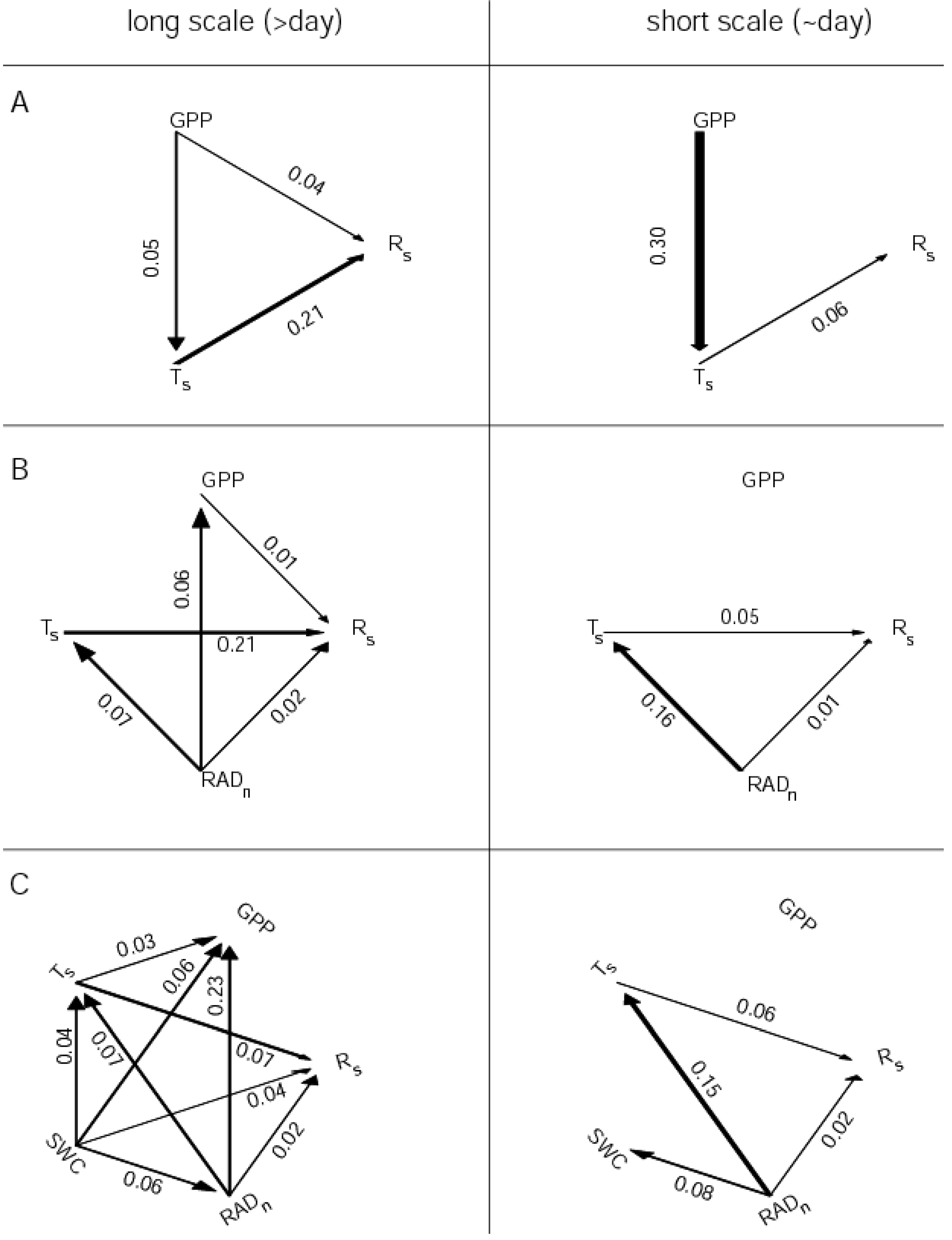
4.2. Direct Connectivity Diagram

Cause-and-effect diagrams can be built based on the outcome of the multivariate G-causality analysis. Each variable is represented as a node of a circular network and significant causal interactions are depicted with arrows pointing in the direction of the influenced variable and its width proportional to the intensity of the interaction. To construct such a diagram we follow two rules:
(1)
Only direct causal interactions are depicted. This implies that if the bivariate interaction is significant, but the multivariate is not, an arrow is not drawn. However, if the bivariate G-causality is not significant, no further action is taken.
(2)
If both directional interactions are detected among two nodes, only the greater is retained.
The spectral G-causality allows creation of connectivity diagrams at different frequencies or averaged in specific bands.

5. Results

Automated soil respiration measurements in the control plot were consistent with those of long-term point measurements [49]. Findings from the present study demonstrate that the treatment site had lower Rs than the control site for all years (Figure 3).
Bivariate and conditional G-causalities on GPP and Ts over Rs showed a large effect of temperature and a much smaller effect of GPP, especially at low frequencies (Figure 4). At daily frequency, and in minor extent at the corresponding half day sub-harmonic, the effect of GPP on Rs appears to be important, although it is largely reduced when Ts is included in the analysis. There are no apparent differences between the two sites in response to temperature and/or GPP. This hypothesis was tested computing the difference Entropy 15 04266 i012
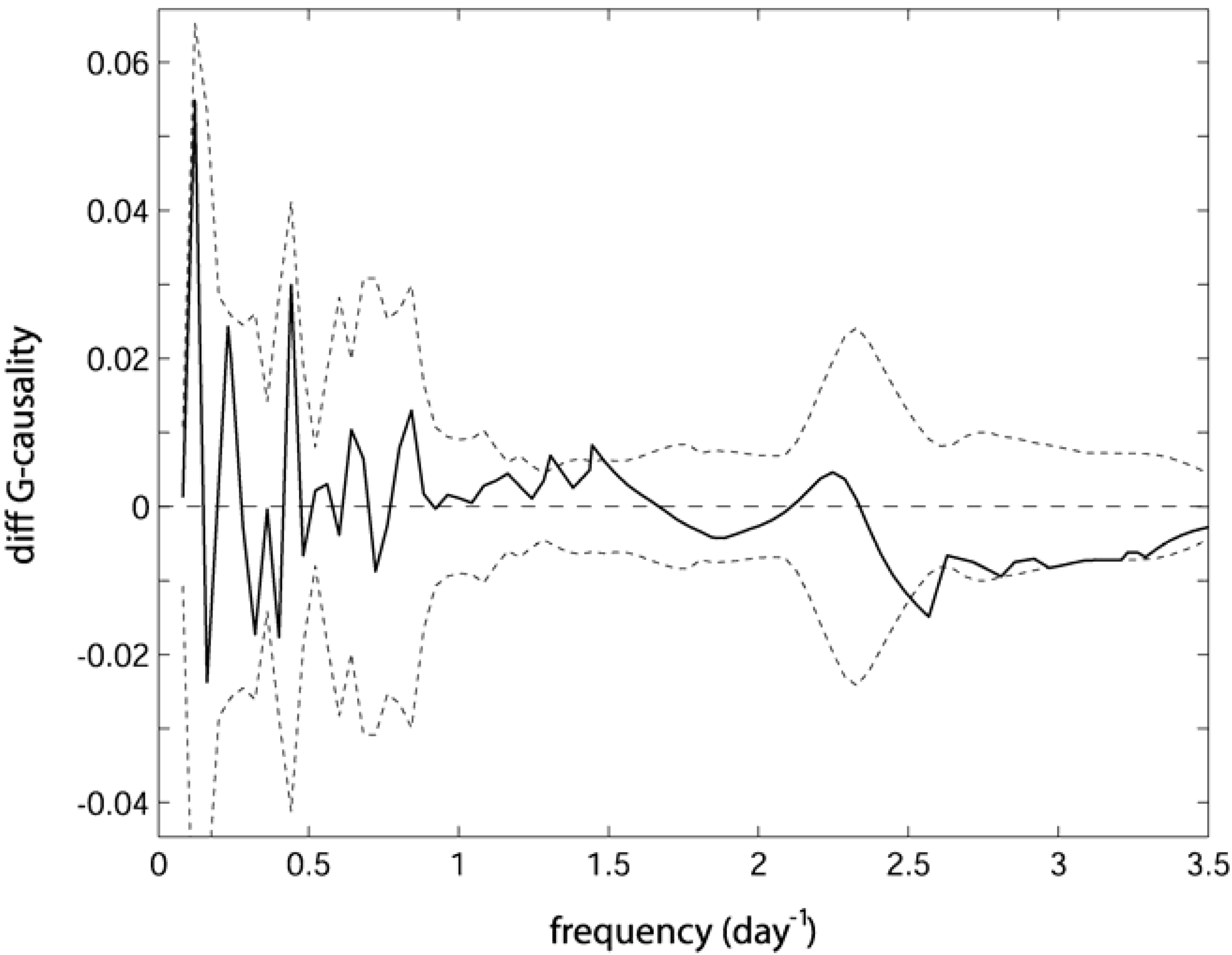
. Confidence intervals obtained upon bootstrapping showed that the differences were not significant (Figure 5).
The analyses were more complicated when other variables were progressively included. To synthetize the results we aggregated the G-causalities in either long time scales (0.2 < frequency < 0.7625 day−1) and short time scales (0.7625 < frequency < 1.7 day−1). Given the fact that the results in both sites were very similar, we also aggregated the data without differentiating among sites. The connectivity graphs (Figure 5) depict only significant direct interactions, i.e., not mediated by other variables.
Figure 4. Bivariate (dashed lines) and conditional (thick lines) G-causalities of GPP and Ts over Rs. Top panels represent control (AmeriFlux) and bottom panels, treatment (FASET). The thick lines represent the desired goal of the analysis because they isolate direct effects, while the dashed lines indicate the apparent connections which are due to a combination of direct and indirect effects.
Entropy 15 04266 g004
Figure 5. Difference of conditional G-causalities of GPP given Ts over Rs between control (AmeriFlux) and treatment (FASET). Dashed lines are the 95th quantiles obtained boostrapping the 60 days blocks of the pulled dataset and divide them in two random groups.
Entropy 15 04266 g005
Figure 6. Connectivity diagram based on the significant direct G-causalities using (A) three, (B) four or (C) five multivariate systems. The widths and values on the arrows indicate average G-causalities for long time scale (0.2 < frequency < 0.7625 day−1) and short time scales (0.7625 < frequency < 1.7 day−1).
Entropy 15 04266 g006
We consider three cases. In the first case only GPP, Rs and Ts are included. This diagram supports the hypothesis of GPP control over Rs at long time scales, though at short time scales a significant interaction cannot be detected (Figure 6A). Note the biologically improbable interaction of GPP over Ts especially at short time scales.
In the second case RADn also is included in the analysis (Figure 6B). Introducing this variable changes the causality pattern slightly. The causal effect of GPP over Rs can still be detected at long scales, although considerably reduced. The causality of GPP over Ts, however, disappears and RADn influences all variables at all time-scales, except for GPP at short scale. This makes sense, as RADn controls all energy processes and is closely coupled with biological processes such as GPP. The disappearance of the influence of GPP on Ts, which was previously detected, indicated that GPP influences Ts indirectly through an unmeasured variable not included in the 3-variable analysis, and most probably RADn. The lack of G-causality of RADn over GPP at short scales can be explained by the fact that radiation influences GPP almost instantaneously, while G-causality only detects lagged responses at the time-scale of the measurements, here—one hour.
In the third case, soil water content was introduced (SWC) (Figure 6C). At short time scale the scheme of interactions does not change as SWC does not act at daily or higher frequencies. However, at long time scales, a complex pattern of casual interactions emerges. RADn and SWC largely control all other variables and the influence of GPP over Rs is lost. Interestingly, SWC is not influenced by any of the other variables, i.e., SWC is Granger autonomous while RADn is influenced by SWC.

6. Discussion

Soil respiration rates and the contribution of this flux to Rs varies considerably among forest types, though the fundamental variables regulating carbon cycling process rates are generally conserved across ecosystems [53]. In the mixed deciduous forests of Michigan, USA, respiration from soils is the largest component of ecosystem respiration, comprising approximately 70% of the total flux of CO2 [30]. Ecological transitions and regional climatic changes can affect Rs. Carbon sequestration by an ecosystem is determined as a small difference between two large fluxes: respiration, which emits CO2 to the atmosphere and gross primary productivity (GPP) that takes up CO2 from the atmosphere through the process of photosynthesis. The small difference between these two opposing fluxes makes the net CO2 sequestration rate highly sensitive to any change in either respiration of GPP.
These climatic changes have motivated the scientific community to quantify Rs and to better understand the factors controlling it, particularly during and after disturbance [54]. Primary climatic controls on Rs are temperature, solar radiation, and precipitation [55]. Soil respiration increases as soil temperatures rise, because microbial community abundance and activity both respond positively to warming [27,56]. Drought and extremely wet conditions limit microbial activity and decrease respiration [57]. Over periods of hours to days, photosynthetic activity also controls carbohydrate supply from leaves to roots resulting in increased C availability to mycorrhizal fungi and microorganisms in the root environment (rhizosphere), thereby increasing Rs [58,59,60,61].
Forest disturbance can change the rates of photosynthetic activity through a reduction in live leaf area and thus GPP, and resulting in changes the soil’s energy budget as temperature and humidity shift in response to reduced shading and water uptake by trees. Disturbance also changes canopy structure and the sub-canopy environment in ways that may affect Rs, modifying light and nutrient use efficiency [62], roughness length, canopy-atmosphere coupling, and increasing turbulence mixing above the soil [63,64]. In both 2008 and 2009 respiration was lower in the treatment site than in the control. Due to the lack of respiration measurements prior to the girdling treatment we cannot rule out that this difference is a result of the treatment.
However, the difference in respiration between the sites was rather constant over the period from 3 months to a year and a half past the treatment, despite stem girdling and eventual and slow mortality (trees where fully alive in summer 2008, and mostly dead in 2009) of canopy dominant trees that occupied roughly 30% of the canopy in 2008. Additionally, the dynamics and causality structure of the drivers of respiration in both sites was not different. Given these two indications, it seems unlikely that that difference is a result of the treatment. This was not because of an ineffective treatment. In summer 2009 the aspen and birch trees were visibly defoliated. However our study indicates resilience of ecosystem functioning to moderate disturbance, and particularly the soil ecosystem which maintained high respiration rates despite a reduction of photosynthates from girdled trees. In part, this resilience is due to compensatory growth and increased productivity of the remaining un-girdled trees from increased light and nitrogen availability [65]. Alternatively, soil respiration may have declined in the treatment very abruptly following the 2008 girdling, shortly before our chamber measurement started. Several studies document an almost immediate decline in Rs that reaches its lowest point within days following stem girdling [54,66], suggesting that the exhaustion of stored labile carbohydrates progressively limits root and rhizosphere respiration.
Our G-causality analysis suggested that GPP did not directly control Rs in either treatment or control site, and that RADn was a primary environmental constraint on Rs through its effects on Ts at short time scales. At longer scale, both SWC and RADn controlled Rs. This finding is similar to other studies suggesting no diurnal relationship between GPP and Rs [67] and in contrast to others showing that GPP or photosynthesis constrains Rs over diurnal timescales [15,58,59,68]. Respiration from our sites is principally limited by soil moisture and radiation (heat to the soil), suggesting that RADn, which is remotely sensed with high accuracy, may serve as a useful predictor of Rs. In another site, the Duke Forest, where a significant link between GPP and Rs was established [15], moisture and temperature were less limiting factors.
Furthermore, under natural conditions, there is a substantial attenuation of the diurnal amplitude of photosynthesis along the phloem path length, primarily influenced by vegetation height and phloem conductivity [69]. At this site, trees were quite tall (around 25 m). Unfortunately, information about phloem conductivity was not available.
Several studies have shown that recently produced photosynthate is a key driver of root respiration and thus, girdling will typically decrease soil respiration [54,66]. Species-specific responses to girdling can be highly variable [70] and in some cases, no effect of girdling on soil respiration was reported [71]. Studies of respiration in pest-infected forests, where the trees were girdled by insects, found mixed results from no effect whatsoever, to a large decline [72,73].
Other methods for testing GPP and Rs interactions were reviewed [60]. Among non-manipulative approaches, methods based on time series analyses, such as cross-correlation, pulse-response and Fourier decomposition, were suggested to detect lagged response. However, we note that only G-causality is able to provide a directionality of the interactions, which is the real signature of a causal mechanism. Furthermore, the multivariate approach investigated in this study showed that including more biophysical factors may reveal indirect or apparent interactions that, in lower dimension systems, may appear as direct and significant. However, the proposed method has also some limitations. Long, continuous and multiple time series are required to construct robust spectral matrices and reduce noise. Although G-causality is less sensitive to random Gaussian noise, other non-Gaussian source of error (e.g., spikes) may cause unpredictable effects. Any additional variable that contains such errors may reduce the statistical power to the extent that weak interactions may not be detectable.

Acknowledgments

We thank Ha-Pe Schmid and Danilo Dragoni that participated in the design and the initial deployment of the soil respiration chambers. The UMBS flux site is funded by the U.S. Department of Energy's Office of Science (BER) project #DE-SC0006708. Soil moisture measurements were funded by NSF grant #DEB-0911461. Kyle Maurer was funded by an IGERT fellowship (NSF grant #DGE-0504552) awarded by the University of Michigan Biosphere-Atmosphere Research Training (BART) program. Matteo Detto was supported by the Smithsonian Institution Global Earth Observatories (SIGEO). Any opinions, findings, and conclusions or recommendations expressed in this material are those of the authors and do not necessarily reflect the views of the National Science Foundation.

Conflicts of Interest

The authors declare no conflict of interest.

References

  1. Melillo, J.M.; Butler, S.; Johnson, J.; Mohan, J.; Steudler, P.; Lux, H.; Burrows, E.; Bowles, F.; Smith, R.; Scott, L.; et al. Soil warming, carbon-nitrogen interactions, and forest carbon budgets. Proc. Natl. Acad. Sci. USA 2011, 108, 9508–9512. [Google Scholar] [CrossRef] [PubMed]
  2. Bond-Lamberty, B.; Thomson, A. Temperature-associated increases in the global soil respiration record. Nature 2010, 464, 579–582. [Google Scholar] [CrossRef] [PubMed]
  3. Canadell, J.G.; Le Quéré, C.; Raupach, M.R.; Field, C.B.; Buitenhuis, E.T.; Ciais, P.; Conway, T.J.; Gillett, N.P.; Houghton, R.A.; Marland, G. Contributions to accelerating atmospheric CO2 growth from economic activity, carbon intensity, and efficiency of natural sinks. Proc. Natl. Acad. Sci. USA 2007, 104, 18866–70. [Google Scholar] [CrossRef] [PubMed]
  4. Fierer, N.; Strickland, M.S.; Liptzin, D.; Bradford, M.A.; Cleveland, C.C. Global patterns in belowground communities. Ecol. Lett. 2009, 12, 1238–1249. [Google Scholar] [CrossRef] [PubMed]
  5. Brutsaert, W. Evaporation into the Atmosphere: Theory, History, and Applications; Springer: Dordrecht, The Netherlands and Boston, MA, USA, 1982; p. 316. [Google Scholar]
  6. Shipley, B. Cause and Correlation in Biology; Cambridge University Press: Cambridge, UK, 2000; p. 317. [Google Scholar]
  7. Wiener, N. The Theory of Prediction. In Modern Mathematics for Engineers; Beckenbach, E.F., Ed.; McGraw-Hill: New York, NY, USA, 1956; Volume 1, pp. 165–183. [Google Scholar]
  8. Barnett, L.; Barrett, A.; Seth, A. Granger causality and transfer entropy are equivalent for Gaussian variables. Phys. Rev. Lett. 2009, 103, 238701. [Google Scholar] [CrossRef] [PubMed]
  9. Hlavácková-Schindler, K. Equivalence of Granger causality and transfer entropy: A generalization. Appl. Math. Sci. 2011, 5, 3637–3648. [Google Scholar]
  10. Granger, C.W.J. Some recent developments in a concept of causality. J. Econom. 1988, 39, 199–211. [Google Scholar] [CrossRef]
  11. Granger, C.W.J. Investigating causal relations by econometric models and cross-spectral methods. Econometrica 1969, 37, 424–438. [Google Scholar] [CrossRef]
  12. Salvucci, G.D.; Saleem, J.A.; Kaufmann, R. Investigating soil moisture feedbacks on precipitation with tests of Granger causality. Adv Water Resour. 2002, 25, 1305–1312. [Google Scholar] [CrossRef]
  13. Kaufmann, R.K.; Paletta, L.F.; Tian, H.Q.; Myneni, R.B.; D’Arrigo, R.D. The power of monitoring stations and a CO2 fertilization effect: Evidence from causal relationships between NDVI and carbon dioxide. Earth Interact. 2008, 12, 1–23. [Google Scholar]
  14. Smirnov, D.A.; Mokhov, I.I. From Granger causality to long-term causality: Application to climatic data. Phys. Rev. E 2009, 80, 016208. [Google Scholar] [CrossRef]
  15. Detto, M.; Molini, A.; Katul, G.; Stoy, P.; Palmroth, S.; Baldocchi, D. Causality and persistence in ecological systems: A nonparametric spectral Granger causality approach. Am. Nat. 2012, 179, 524–535. [Google Scholar] [CrossRef] [PubMed]
  16. Kumar, P.; Ruddell, B.L. Information driven ecohydrologic self-organization. Entropy 2010, 12, 2085–2096. [Google Scholar] [CrossRef]
  17. Ruddell, B.L.; Kumar, P. Ecohydrologic process networks: 2. Analysis and characterization. Water Resour. Res. 2009, 45. [Google Scholar] [CrossRef]
  18. Geweke, J. Measurement of linear dependence and feedback between multiple time series. J. Am. Stat. Assoc. 1982, 77, 304–313. [Google Scholar] [CrossRef]
  19. Dhamala, M.; Rangarajan, G.; Ding, M. Estimating Granger causality from Fourier and wavelet transforms of time series data. Phys. Rev. Lett. 2008, 100, 1–4. [Google Scholar] [CrossRef]
  20. Baldocchi, D.; Falge, E.; Wilson, K. A spectral analysis of biosphere–atmosphere trace gas flux densities and meteorological variables across hour to multi-year time scales. Agricul. For. Meteorol. 2001, 107, 1–27. [Google Scholar] [CrossRef]
  21. Katul, G.; Lai, C.; Schäfer, K. Multiscale analysis of vegetation surface fluxes: From seconds to years. Adv. Water Resour. 2001, 24, 1119–1132. [Google Scholar] [CrossRef]
  22. Hatala, J.A.; Detto, M.; Baldocchi, D.D. Gross ecosystem photosynthesis causes a diurnal pattern in methane emission from rice. Geophys. Res. Lett. 2012, 39. [Google Scholar] [CrossRef]
  23. Kilburn, P.D. Effects of logging and fire on xerophytic forests in northern Michigan. Bull. Torrey Bot. Club 1960, 87, 402–405. [Google Scholar] [CrossRef]
  24. Nave, L.E.; Gough, C.M.; Maurer, K.D.; Bohrer, G.; Hardiman, B.S.; Le Moine, J.; Munoz, A.B.; Nadelhoffer, K.J.; Sparks, J.P.; Strahm, B.D.; et al. Disturbance and the resilience of coupled carbon and nitrogen cycling in a north temperate forest. J. Geophys. Res. Biogeosci. 2011, 116. [Google Scholar] [CrossRef]
  25. Stoy, P.C.; Palmroth, S.; Oishi, A.C.; Siqueira, M.B.S.; Juang, J.-Y.; Novick, K.A.; Ward, E.J.; Katul, G.G.; Oren, R. Are ecosystem carbon inputs and outputs coupled at short time scales? A case study from adjacent pine and hardwood forests using impulse-response analysis. Plant Cell Environ. 2007, 30, 700–710. [Google Scholar] [CrossRef] [PubMed]
  26. Martin, J.; Phillips, C.; Schmidt, A.; Irvine, J.; Law, B. High-frequency analysis of the complex linkage between soil CO2 fluxes, photosynthesis and environmental variables. Tree Physiol. 2012, 32, 49–64. [Google Scholar] [CrossRef] [PubMed]
  27. Bouma, T.; Nielsen, K.; Eissenstat, D.; Lynch, J. Estimating respiration of roots in soil: interactions with soil CO2, soil temperature and soil water content. Plant Soil 1997, 195, 221–232. [Google Scholar] [CrossRef]
  28. Nave, L.; Vogel, C. Contribution of atmospheric nitrogen deposition to net primary productivity in a northern hardwood forest. Can. J. For. Res. 2009, 39, 1108–1118. [Google Scholar] [CrossRef]
  29. MatLab, version 7.6.0 R2008a; software for technical computation, Mathworks: Natick, MA, USA, 2008.
  30. Curtis, P.S.; Vogel, C.S.; Gough, C.M.; Schmid, H.P.; Su, H.-B.; Bovard, B.D. Respiratory carbon losses and the carbon-use efficiency of a northern hardwood forest, 1999-2003. New Phytol. 2005, 167, 437–455. [Google Scholar] [CrossRef] [PubMed]
  31. Lee, X.J.; Finnigan, J.; Paw U, K.T. Coordinate Systems and Flux Bias Error. In Handbook of Micrometeorology, a Guide for Surface Flux Measurement and Analysis; Lee, X., Massman, W., Law, B., Eds.; Kluwer Academic: Dordrecht, The Netherlands, 2004; pp. 33–66. [Google Scholar]
  32. Massman, W.J. A simple method for estimating frequency response corrections for eddy covariance systems. Agricul. For. Meteorol. 2000, 104, 185–198. [Google Scholar] [CrossRef]
  33. Schotanus, P.; Nieuwstadt, F.T.M.; Bruin, H.A.R. Temperature measurement with a sonic anemometer and its application to heat and moisture fluxes. Bound.-Layer Meteorol. 1983, 26, 81–93. [Google Scholar] [CrossRef]
  34. Liu, H.; Peters, G.; Foken, T. New equations for sonic temperature variance and buoyancy heat flux with an omnidirectional sonic anemometer. Bound.-Layer Meteorol. 2001, 100, 459–468. [Google Scholar] [CrossRef]
  35. Kaimal, J.C.; Gaynor, J.E. Another look at sonic thermometry. Bound.-Layer Meteorol. 1991, 56, 401–410. [Google Scholar] [CrossRef]
  36. Munger, J.W.; Loescher, H.W. Guidelines For Making Eddy Covariance Flux Measurements, 2009. Available online: http://public.ornl.gov/ameriflux/measurement_standards_020209.doc (accessed on 5 October 2013).
  37. Webb, E.K.; Pearman, G.I.; Leuning, R. Correction of flux measurements for density effects due to heat and water vapour transfer. Quart. J. Roy. Meteorol. Soc. 1980, 106, 85–100. [Google Scholar] [CrossRef]
  38. Detto, M.; Katul, G.G. Simplified expressions for adjusting higher-order turbulent statistics obtained from open path gas analyzers. Bound.-Layer Meteorol. 2007, 122, 205–216. [Google Scholar] [CrossRef]
  39. Garrity, S.R.; Bohrer, G.; Maurer, K.D.; Mueller, K.L.; Vogel, C.S.; Curtis, P.S. A comparison of multiple phenology data sources for estimating seasonal transitions in deciduous forest carbon exchange. Agricul. For. Meteorol. 2011, 151, 1741–1752. [Google Scholar] [CrossRef]
  40. Reichstein, M.; Falge, E.; Baldocchi, D.; Papale, D.; Aubinet, M.; Berbigier, P.; Bernhofer, C.; Buchmann, N.; Gilmanov, T.; Granier, A.; et al. On the separation of net ecosystem exchange into assimilation and ecosystem respiration: review and improved algorithm. Glob. Change Biol. 2005, 11, 1424–1439. [Google Scholar] [CrossRef]
  41. Papale, D.; Reichstein, M.; Aubinet, M.; Canfora, E.; Bernhofer, C.; Kutsch, W.; Longdoz, B.; Rambal, S.; Valentini, R.; Vesala, T.; et al. Towards a standardized processing of net ecosystem exchange measured with eddy covariance technique: Algorithms and uncertainty estimation. Biogeosciences 2006, 3, 571–583. [Google Scholar] [CrossRef]
  42. Schmid, H.P. Ecosystem-atmosphere exchange of carbon dioxide over a mixed hardwood forest in northern lower Michigan. J. Geophys. Res. 2003, 108. [Google Scholar] [CrossRef]
  43. Lasslop, G.; Migliavacca, M.; Bohrer, G.; Reichstein, M.; Bahn, M.; Ibrom, A.; Jacobs, C.; Kolari, P.; Papale, D.; Vesala, T.; et al. On the choice of the driving temperature for eddy-covariance carbon dioxide flux partitioning. Biogeosciences 2012, 9, 5243–5259. [Google Scholar] [CrossRef]
  44. Papale, D.; Valentini, R. A new assessment of European forests carbon exchanges by eddy fluxes and artificial neural network spatialization. Glob. Change Biol. 2003, 9, 525–535. [Google Scholar] [CrossRef]
  45. Detto, M.; Montaldo, N.; Albertson, J.D.; Mancini, M.; Katul, G. Soil moisture and vegetation controls on evapotranspiration in a heterogeneous Mediterranean ecosystem on Sardinia, Italy. Water Resour. Res. 2006, 42. [Google Scholar] [CrossRef]
  46. Chen, B.; Black, T.A.; Coops, N.C.; Hilker, T.; Trofymow, J.A.; Morgenstern, K. Assessing tower flux footprint climatology and scaling between remotely sensed and eddy covariance measurements. Bound.-Layer Meteorol. 2008, 130, 137–167. [Google Scholar] [CrossRef]
  47. Masani, P. Recent Trends in Multivariate Prediction Theory. In Multivariate Analysis, Proceedings of International Symposium on Multivariate Analysis, Dayton, OH, USA, 1965; Academic Press: New York, NY, USA, 1966; pp. 351–382. [Google Scholar]
  48. Chen, Y.; Bressler, S.L.; Ding, M. Frequency decomposition of conditional Granger causality and application to multivariate neural field potential data. J. Neurosci. Methods 2006, 150, 228–37. [Google Scholar] [CrossRef] [PubMed]
  49. Hlavackova-Schindler, K.; Paluš, M.; Vejmelkab, M.; Bhattacharya, J. Causality detection based on information-theoretic approaches in time series analysis. Phys. Rep. 2007, 441, 1–46. [Google Scholar] [CrossRef]
  50. Masani, P. Wiener’s contribution to generalized harmonic analysis prediction theory and filter theory. Bull. Am. Math. Soc. 1966, 72, 73–125. [Google Scholar] [CrossRef]
  51. Wilson, G. The factorization of matricial spectral densities. SIAM J. Appl. Math. 1972, 23, 420–426. [Google Scholar] [CrossRef]
  52. Schreiber, T.; Schmitz, A. Surrogate time series. Physica D 2000, 142, 346–382. [Google Scholar] [CrossRef]
  53. Hibbard, K.A.; Law, B.E.; Reichstein, M.; Sulzman, J. An analysis of soil respiration across northern hemisphere temperate ecosystems. Biogeochemistry 2005, 73, 29–70. [Google Scholar] [CrossRef]
  54. Levy-Varon, J.H.; Schuster, W.S.F.; Griffin, K.L. The autotrophic contribution to soil respiration in a northern temperate deciduous forest and its response to stand disturbance. Oecologia 2012, 169, 211–220. [Google Scholar] [CrossRef] [PubMed]
  55. Ryan, M.G.; Law, B.E. Interpreting, measuring, and modeling soil respiration. Biogeochemistry 2005, 73, 3–27. [Google Scholar] [CrossRef]
  56. Elberling, B. Seasonal trends of soil CO2 dynamics in a soil subject to freezing. J. Hydrol. 2003, 276, 159–175. [Google Scholar] [CrossRef]
  57. Lin, Z.; Zhang, R.; Tang, J.; Zhang, J. Effects of high soil water content and temperature on soil respiration. Soil Sci. 2011, 176, 150–155. [Google Scholar] [CrossRef]
  58. Braswell, B.; Sacks, W. Estimating diurnal to annual ecosystem parameters by synthesis of a carbon flux model with eddy covariance net ecosystem exchange observations. Glob. Change Biol. 2005, 11, 335–355. [Google Scholar] [CrossRef]
  59. Kodama, N.; Barnard, R.L.; Salmon, Y.; Weston, C.; Ferrio, J.P.; Holst, J.; Werner, R.A.; Saurer, M.; Rennenberg, H.; Buchmann, N.; Gessler, A. Temporal dynamics of the carbon isotope composition in a Pinus sylvestris stand: From newly assimilated organic carbon to respired carbon dioxide. Oecologia 2008, 156, 737–750. [Google Scholar] [CrossRef] [PubMed]
  60. Kuzyakov, Y.; Gavrichkova, O. Review: Time lag between photosynthesis and carbon dioxide efflux from soil: A review of mechanisms and controls. Glob. Change Biol. 2010, 16, 3386–3406. [Google Scholar] [CrossRef]
  61. Werner, C.; Gessler, A. Diel variations in the carbon isotope composition of respired CO2 and associated carbon sources: A review of dynamics and mechanisms. Biogeosciences 2011, 8, 2437–2459. [Google Scholar] [CrossRef]
  62. Hardiman, B.S.; Bohrer, G.; Gough, C.M.; Vogel, C.S.; Curtis, P.S. The role of canopy structural complexity in wood net primary production of a maturing northern deciduous forest. Ecology 2011, 92, 1818–1827. [Google Scholar] [CrossRef] [PubMed]
  63. Bohrer, G.; Katul, G.; Walko, R.; Avissar, R. Exploring the effects of microscale structural heterogeneity of forest canopies using large-eddy simulations. Bound.-Layer Meteorol. 2009, 132, 351–382. [Google Scholar] [CrossRef]
  64. Maurer, K.D.; Hardiman, B.S.; Vogel, C.S.; Bohrer, G. Canopy-structure effects on surface roughness parameters: Observations in a Great Lakes mixed-deciduous forest. Agricul. For. Meteorol. 2013, 177, 24–34. [Google Scholar] [CrossRef]
  65. Gough, C.M.; Hardiman, B.S.; Nave, L.; Bohrer, G.; Maurer, K.D.; Vogel, C.S.; Nadelhoffer, K.J.; Curtis, P.S. Sustained carbon uptake and storage following moderate disturbance in a Great Lakes forest. Ecol. Appl. 2013, 23, 1202–1215. [Google Scholar] [CrossRef] [PubMed]
  66. Högberg, P.; Nordgren, A.; Buchmann, N.; Taylor, A.F.; Ekblad, A.; Högberg, M.N.; Nyberg, G.; Ottosson-Löfvenius, M.; Read, D.J. Large-scale forest girdling shows that current photosynthesis drives soil respiration. Nature 2001, 411, 789–92. [Google Scholar] [CrossRef] [PubMed]
  67. Betson, N.R.; Göttlicher, S.G.; Hall, M.; Wallin, G.; Richter, A.; Högberg, P. No diurnal variation in rate or carbon isotope composition of soil respiration in a boreal forest. Tree Physiol. 2007, 27, 749–56. [Google Scholar] [CrossRef] [PubMed]
  68. Tang, J.W.; Baldocchi, D.D.; Xu, L. Tree photosynthesis modulates soil respiration on a diurnal time scale. Glob. Change Biol. 2005, 11, 1298–1304. [Google Scholar] [CrossRef]
  69. Mencuccini, M.; Hölttä, T. The significance of phloem transport for the speed with which canopy photosynthesis and belowground respiration are linked. New Phytol. 2010, 185, 189–203. [Google Scholar] [CrossRef] [PubMed]
  70. Chen, D.; Zhang, Y.; Lin, Y.; Zhu, W.; Fu, S. Changes in belowground carbon in Acacia crassicarpa and Eucalyptus urophylla plantations after tree girdling. Plant Soil 2010, 326, 123–135. [Google Scholar] [CrossRef]
  71. Edwards, N.T.; Ross-Todd, B.M. Effects of stem girdling on biogeochemical cycles within mixed deciduous forest in Eastern Tennessee. 1. Soil solition chamistry, soil respiration, litterfall and root biomass studies. Oecologia 1979, 40, 247–257. [Google Scholar] [CrossRef]
  72. Morehouse, K.; Johns, T.; Kaye, J.; Kaye, A. Carbon and nitrogen cycling immediately following bark beetle outbreaks in southwestern ponderosa pine forests. For. Ecol. Manag. 2008, 255, 2698–2708. [Google Scholar] [CrossRef]
  73. Hicke, J.A.; Allen, C.D.; Desai, A.R.; Dietze, M.C.; Hall, R.J.; Hogg, E.H.; Kashian, D.M.; Moore, D.; Raffa, K.F.; Sturrock, R.N.; et al. Effects of biotic disturbances on forest carbon cycling in the United States and Canada. Glob. Change Biol. 2012, 18, 7–34. [Google Scholar] [CrossRef]

