A Finite-Time Thermal Cycle Variational Optimization with a Stefan–Boltzmann Law for Three Different Criteria

Abstract

This work shows the power of the variational approach for studying the efficiency of thermal engines in the context of the Finite Time Thermodynamics (FTT). Using an endoreversible Curzon–Ahlborn (CA) heat engine as a model for actual thermal engines, three different criteria for thermal efficiency were analyzed: maximum power output, ecological function, and maximum power density. By means of this procedure, the performance of the CA heat engine with a nonlinear heat transfer law (the Stefan–Boltzmann law) was studied to describe the heat exchanges between the working substance and its thermal reservoirs. The specific case of the Müser engine for all the criteria was analyzed. The results confirmed some previous findings using other procedures and additionally new results for the Müser engine performance were obtained.

1. Introduction

Several authors [1,2,3,4,5,6,7,8,9] have pointed out that endoreversible thermal cycle models working in maximum power conditions have an efficiency that strongly depends on the heat transfer law used to describe the heat fluxes between the working fluid and its surroundings. In fact, one of the most impressive results of the Curzon–Alhborn (CA) paper [10] was that the authors found very reasonable numerical results for the efficiency of certain power plants by means of a very simple formula for a Carnot-like finite time heat engine in a maximum power output regime but where a linear heat transfer law was used. Since the CA paper, many authors have considered more realistic models to describe the heat exchanges using non-linear heat transfer laws [1,2,3,4,5,6,7,8,9,10,11,12,13,14,15,16,17,18,19,20,21]. Generally, the quantities to optimize are functionals such as work, power output and entropy production or a combination of these, which can be expressed as integrals over certain trajectories.

Thus, it becomes natural to use the variational calculus to treat optimization problems such as the ones mentioned previously. For instance, in the CA paper the equation that represents the thermal cycle efficiency was found by the maximization of the power output as a two variable function $P=P(x,y)$ with $x=T_H-T_h$ and $y=T_L-T_l$, where $T_H$ and $T_L$ represent the absolute temperatures of the hot and cold reservoirs respectively (see Figure 1).

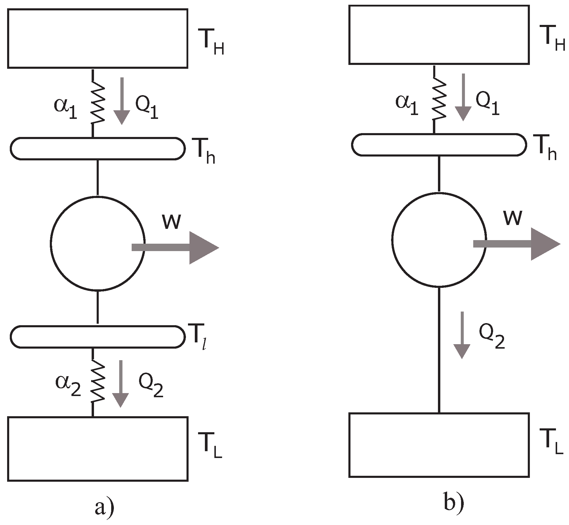
Figure 1. (a) Diagram of the CA endoreversible heat engine with conductances ${\alpha }_1={\alpha }_2=\alpha$; (b) The Müser engine.

Figure 1. (a) Diagram of the CA endoreversible heat engine with conductances ${\alpha }_1={\alpha }_2=\alpha$; (b) The Müser engine.

In fact, Rubin [22] could obtain the CA engine efficiency through the maximization of the Lagrangian with the power output as the objective function and the endoreversibility condition as the integral restriction. It is worth noting that in the later case the authors use a linear heat transfer law as CA did. Later Ares de Parga et al. [23,24] used the variational approach to study a CA engine under both maximum power and maximum ecological function conditions [25]. They analyzed the performance of the CA engine with a nonlinear heat transfer law (the Dulong and Petit law [24]), obtaining results consistent with those previously obtained by means of other procedures. In this work, an analysis was made following the same ideas of Ares de Parga et al. [24] but considering a different heat transfer law, namely the Stefan–Boltzmann law, which considers only radiative effects and has not been used before in the variational approach.

In this paper, a variational approach was used to study a CA engine for three different criteria: maximum power output, ecological function and maximum power density, where a heat transfer law different from previous studies was used. Under the maximum power output criterion, it is possible to recover all the numerical results for the Müser engine reported in [26]. Additionally, new outcomes were obtained for the engine efficiency in the special case of the Müser engine, using the two mentioned additional criteria.

The paper is organized as follows. Section 2 presents a brief introduction to previous work about the variational optimization and its application to the cycle’s power output for a CA engine using the maximum power output criterion. Section 3 presents the application of the variational approach to a CA engine under the ecological function criterion. In order to prove the validity of the results, the limit case of a Müser engine is considered. Section 4 presents the maximization of the CA engine using the maximum power density criterion. Finally, in Section 5, we present some concluding remarks.

2. Maximum Power Criterion

In 1975, Curzon and Ahlborn [10] published their paper. The main result was that they could obtain maximum power output efficiency for a finite time Carnot-like thermal engine using a linear heat transfer. This efficiency is shown by the following expression,

$${\eta }_{CA}=1-\sqrt{\frac{T_L}{T_H}}$$

(1)

Later, in 1979, Rubin [22] obtained Equation (1) by means of the variational calculus application for power maximization, treated as the functional subject to the endoreversibility condition as a restriction. Rubin’s approach is based on one of the most important results of classical thermodynamics, which states that the maximum work in thermal process with fixed constraints is obtained when performing a reversible process that leads to upper bounds of performance criteria for an arbitrary process [22]. Taking the above as a starting point, Rubin addresses the following problem in the context of endoreversible thermodynamics. For a CA engine, which is the maximum work output W per cycle subject to the constraint $\Delta S_w=0$?, this means that the entropy changes of the working fluid in one period is zero.

For this purpose, Rubin considered that in the CA engine, the work performance by the engine in one cycle is given by

$$W={\int }_0^{\tau }p\dot{v}dt$$

(2)

where p and v are the pressure and volume of the working fluid. Applying the first law of thermodynamics, $\dot{q}=\dot{u}+p\dot{v}$, where $\dot{q}$ is the heat flux and, substituting it in Equation (2), we obtain,

$$W={\int }_0^{\tau }\dot{q}dt$$

(3)

It can be observed that W is a functional (functionals are often expressed as definite integrals involving functions and their derivatives). If we desire to locate the extrema of functionals, as is in our case, we need to use the calculus. Therefore, mathematically, we seek functions $f\left(x\right)$ that extremize the integral of a function $\mathit{L}(f\left(x\right),f^{\prime }\left(x\right),x)$. The solutions to this problem can be shown to satisfy the Euler–Lagrange equations [27]. We proceed as in ordinary calculus. First, we write the constraint as a function equal to zero, $\Delta S_w=0$. Second, we add this term to the function $\mathit{L}$ times by $\lambda \left(t\right)$:

$$\mathit{L}\lambda (f\left(x\right),f^{\prime }\left(x\right),x,\lambda )=L(f\left(x\right),f^{\prime }\left(x\right),x)+\lambda \Delta S$$

(4)

In this case, $\mathit{L}(f\left(x\right),f^{\prime }\left(x\right),x)=W$ $={\int }_0^{\tau }p\dot{v}dt$, so finally we obtain the new function $\mathit{L}\lambda (f\left(x\right),f^{\prime }\left(x\right),x)$ or simply $\mathit{L}$ as,

$$\mathit{L}=W+\lambda \Delta S_w$$

(5)

where λ is a Lagrange multiplier and $\Delta S_w=0$ is the endoreversible condition, given by

$$\Delta S_W={\int }_0^{\tau }\frac{\dot{q}}{T}dt$$

(6)

where T is the working substance temperature and t is the time. Now assuming a heat transfer law of the form

$$\dot{q}=\alpha (T_R^n-T^n)$$

(7)

where α is the thermal conductance and $T_R$ is the heat reservoir temperature. Taking into account the explicit form of Equation (7) we have

$$L={\int }_0^{\tau }\left[\alpha (T_R^n-T^n)-\lambda \alpha \frac{(T_R^n-T^n)}{T}\right]dt$$

(8)

where the local equilibrium condition for the first law of thermodynamics was used. Following Rubin’s procedure, setting the first variation of Equation (5) equal to zero, we have

$$\delta L={\int }_0^{\tau }\left[\delta T_{R}g(T,T_R,T_L,\lambda )-\delta Tf(T,T_R,T_L,\lambda )\right]dt=0$$

(9)

where

$$g(T,T_R,T_L,\lambda )=T_R^{n-1}(1-\frac{\lambda }{T})$$

and

$$f(T,T_R,T_L,\lambda )=T^{n-1}(\frac{\lambda }{T}-1)$$

Equation (9) has the same form as Equation (24) of [23]. Since $T_R$ is necessarily in the interval $T_L\le T_R\le T_H$, this is a unilateral restriction [2]. Thus, the variation of $\delta T_R$ will not correspond to a physical situation and then only $T_R=T_L$ or $T_R=T_H$ is considered. Therefore, in this analysis, $T_R$ assumes a fixed value of $T_H$ or $T_L$. Finally, from Equation (9) we obtain

$$-n{T}^{n+1}+\lambda T^n(n-1)+\lambda T_R^n=0$$

(10)

In order to verify Equation (10), the special case when $n=1$ is considered, which gives

$$T^2-\lambda T_R=0$$

(11)

Set $T_R=T_H$ and $T=T_h$ or $T=T_l$, we have

$${\eta }_{CA}=1-\sqrt{\frac{T_L}{T_H}}$$

(12)

This equation is consistent with the CA case, in the limit $n=1$. Now, returning to Equation (10) but using the Stefan–Boltzmann nonlinear heat transfer law where $n=4$, Equation (10) takes the following form,

$$4T^5-3\lambda T^4-\lambda T_R^4=0$$

(13)

As in the previous case, $T_R=T_H$ and $T=T_h$ or $T=T_l$ can be assumed, which implies that

$$4T_h^5-3\lambda T_h^4-\lambda T_H^4=0$$

(14)

and

$$4T_l^5-3\lambda T_l^4-\lambda T_L^4=0$$

(15)

Equations (14) and (15) need to be solved to give $T_h$ or $T_l$ respectively and then to derive the endoreversible efficiency by $\eta =1-T_l/T_h$. However, Equations (14) and (15) have no analytical solution. Whereas the solutions of a fourth-degree equation can always be written in terms of radicals, the solutions of an arbitrary fifth-degree polynomial equation cannot. Only some special classes of fifth-degree equations have analytical solutions in terms of nested radicals. Therefore, in order to prove the usefulness of the variational method, an approximation of the Stefan–Boltzmann engine called the Müser engine (ME) [28] introduced by Müser in 1957 can be used. This is a model of the Stefan–Boltzmann engine, which assumes that technology is so good that the conversion device is in a perfect thermal contact with the second reservoir, thus $T_l=T_L$, see Figure 1b. Taking into account this restriction, the Lagrange multiplier λ in Equation (15) now takes the form

$$\lambda =T_l$$

(16)

Now substituting Equation (16) in Equation (14) gives

$$4T_h^5-3T_l{T}_h^4-T_l{T}_H^4=0$$

(17)

This equation is the same to that discovered by Müser [28] in 1957, which was afterwards rediscovered independently by Jeter [29] and by De Vos and Pauwels [30] in 1981. However, here it is obtained by a different method.

Now taking the endoreversible efficiency, $\eta =1-\frac{T_l}{T_h}$, and substituting it into Equation (17), the following expression is shown,

$$T_H^4{(1-\eta )}^5+3T_l^4(1-\eta )-4T_l^4=0$$

(18)

which is the Equation (5.7) obtained by De Vos in his well-known book [26]. Again, as stated before, it has no analytical solution. The numerical solution of Equation (18) for η yields

$${\eta }_{MP}=0.2029$$

(19)

where we take the same approximation as De Vos [26] for the special case of solar converter or Müser engine, that is, $T_l=288$ K and $T_H=431$ K, which are the average planet temperature and the effective sky temperature respectively.

3. Ecological Function Criterion

Many criteria of merit have been proposed for the study of a CA engine. Among these, the maximization of a kind of ecological function [7,25] is found, which consists in the maximization of a function E that represents a relationship between high power output and low entropy production per cycle. This function is given by

$$E=P-T_L\sigma$$

(20)

where P is the power output, σ is the total entropy production (system plus surroundings) per cycle, and $T_L$ is the temperature of the cold reservoir. Alternatively, Yan [31] proposed that it might be more convenient to use $E=P-T_0\sigma$, if the cold reservoir temperature $T_L$ is not equal to the environmental temperature $T_0$, from the exergy analysis point of view.

Ecological function shows two important properties [6,23,25]. Firstly, if a CA engine works in this regime, the thermal efficiency is shown as

$${\eta }_E\approx \frac{1}{2}({\eta }_C+{\eta }_{MP})$$

(21)

where ${\eta }_C$ is the Carnot efficiency and ${\eta }_{MP}$ is the efficiency at maximum power regime.

Secondly, in this regime the CA engine produces around 80% of maximum power, while entropy production is reduced down to around 30% of the entropy produced in the maximum power regime. It has been shown that Equation (21), called the semi-sum property, is independent of the heat transfer law used in the process and is termed as a universal property for the endoreversible systems [6,23].

Taking into account Section 2 and the above, a Lagrangian function L can be proposed as [23],

$$L_E=W-T_L\sigma -\lambda \Delta S_w$$

(22)

where the power output is replaced by the work per cycle W (fixing cycling period τ), σ is the universe entropy production, λ is the Lagrange multiplier and $\Delta S_w=0$ is the endoreversibility constraint in the same way as proposed in Equation (8). Taking the universe entropy production rate in the same mode as Ares de Parga et al. [23] did, but now considering the general heat transfer law Equation (7), we get

$$\sigma =\alpha \left(\frac{T^n-T_R^n}{T_R}\right)$$

(23)

where α is the thermal conductance. Substituting Equations (6), (7) and (23) into (22) yields,

$$L_E={\int }_0^{\tau }\alpha (T_R^n-T^n)-\frac{\alpha \lambda (T_R^n-T^n)}{T}-\frac{T_L}{T_R}\alpha (T^n-T_R^n)$$

(24)

Reorganizing terms then gives

$$L_E={\int }_0^{\tau }\alpha (T_R^n-T^n)\left[1+\frac{T_L}{T_R}-\frac{\lambda }{T}\right]$$

(25)

By setting the first variation of $L_E$ equal to zero, we obtain

$$-n{T}^{n+1}\left(1+\frac{T_L}{T_R}\right)+\lambda T^n(n-1)+\lambda T_R^n=0$$

(26)

This last equation is analogous to Equation (10) but now takes the ecological criterion instead of the maximum power regime. In order to verify Equation (26), an example that has been studied in [23] is taken. For this specific case ($n=1$), Equation (26) yields

$$T^2=\frac{\lambda T_R}{1+T_L/T_R}$$

(27)

In the last equation, the specific case that $T_R=T_H$ and $T=T_h$ gives $T_h={\left(\frac{\lambda T_H}{1+T_L/T_H}\right)}^{1/2}$, which is the same as Equation (27) in [23]. Hence, returning to our case, i.e., taking $n=4$ (Stefan–Boltzmann heat transfer law), Equation (26) gives

$$-4T^5(1+\frac{T_L}{T_R})+3\lambda T^4+\lambda T_R^4=0$$

(28)

Now, as in the previous section, if $T_R=T_H$ and $T=T_h$ then

$$-4T_h^5(1+\frac{T_L}{T_R})+3\lambda T_h^4+\lambda T_H^4=0$$

(29)

and if $T_R=T_L$ and $T=T_l$ then

$$-8T_l^5+3\lambda T_l^4+\lambda T_L^4=0$$

(30)

Equations (29) and (30) need to be solved to give $T_h$ or $T_l$ respectively and then to derive the endoreversible efficiency by $\eta =1-\frac{T_l}{T_h}$. However, Equations (29) and (30) have no analytical solution. Once again, in order to prove the usefulness of the variational method, an approximation of the Stefan–Boltzmann engine called the Müser engine (ME) [28] can be used. This engine considers $T_l=T_L$, as was mentioned before. Taking into account this restriction, from Equation (30) the Lagrange multiplier λ takes the form

$$\lambda =2T_L$$

(31)

Substituting Equation (31) in Equation (29) gives

$$-4T_h^5\left(1+\frac{T_L}{T_H}\right)+6T_L{T}_h^4+2T_L{T}_H^4=0$$

(32)

This equation is similar to that obtained by Müser and by De Vos [26] (Equation (5.7) in his book), but it is obtained for the ecological criterion. It is important to note that this is a new outcome by means of the ecological criterion.

Equation (32) has no analytical solution as mentioned before. However, taking the special case in which $T_L=288$ K and $T_H=431$ K, as in Section 2, we have,

$$T_h=389.04K$$

(33)

Now, taking the endoreversible efficiency, $\eta =1-\frac{T_l}{T_h}$, substitute the values of $T_h$ just obtained and assume $T_l=T_L$. For ${\eta }_E$ we then get

$${\eta }_E=0.2597$$

(34)

Two important facts are noticed. (a) The efficiency for the Müser Stefan–Boltzmann engine is higher in the ecological case than in the maximum power case, as expected. (b) The so-called ecological function has some interesting properties. Among them, the semi-sum property is given in an approximate manner by Equation (21), ${\eta }_E\approx \frac{1}{2}({\eta }_C+{\eta }_{MP})$, where ${\eta }_C$ is the Carnot efficiency and ${\eta }_{MP}$ is the efficiency at the maximum power regime. Using the semi-sum property for our case, in which ${\eta }_C=1-\frac{T_L}{T_H}=0.3317$ and ${\eta }_{MP}=1-\sqrt{\frac{T_L}{T_H}}=0.2029$, we then have ${\eta }_E=0.2673$, which is close to Equation (34).

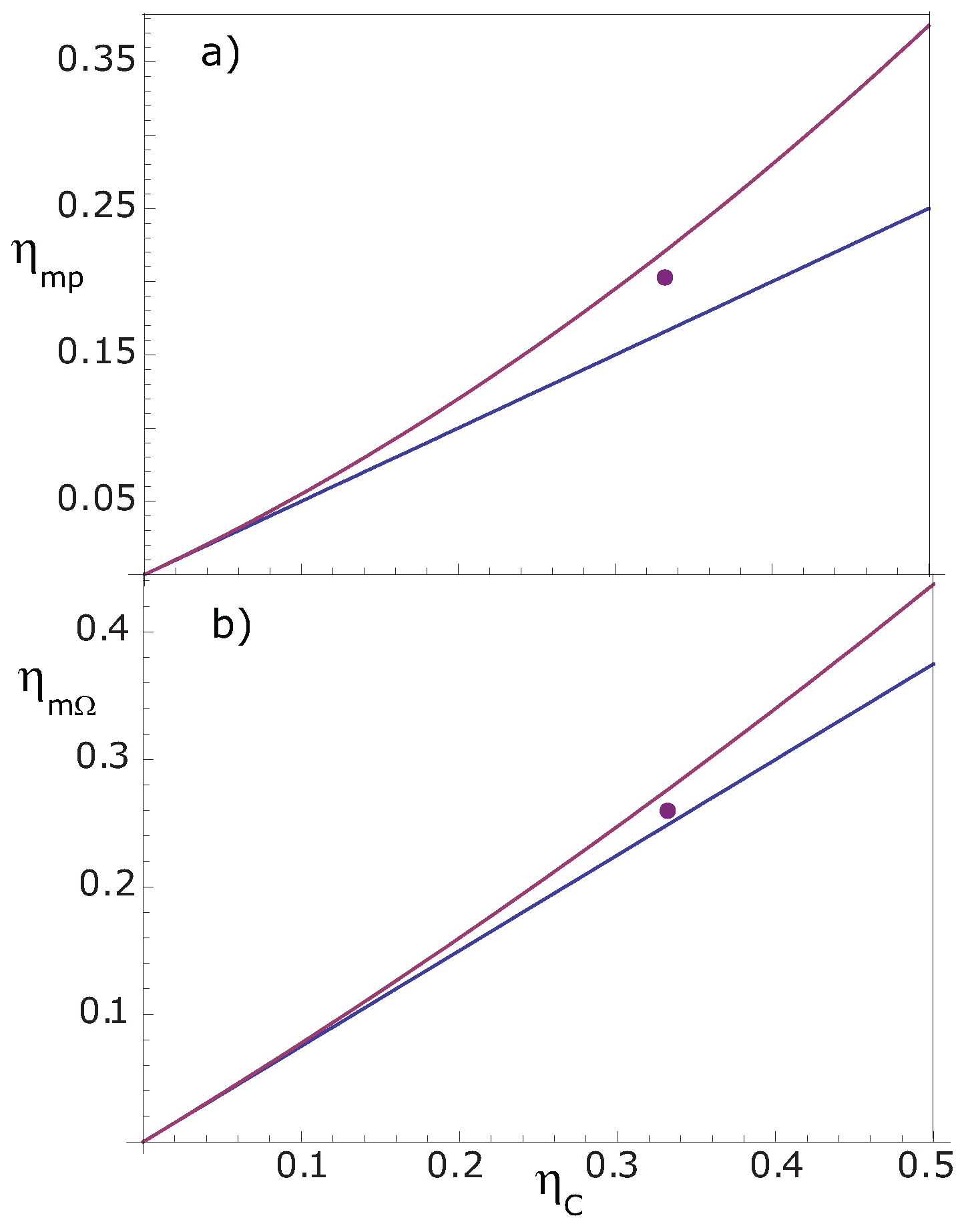
Figure 2. (a) ${\eta }_{MP}$ Equation (19), and the upper and lower bounds for the efficiency at maximum power for systems without symmetry conditions reported in [33]; (b) ${\eta }_E$ Equation (34), bounds for maximum Ω.

Figure 2. (a) ${\eta }_{MP}$ Equation (19), and the upper and lower bounds for the efficiency at maximum power for systems without symmetry conditions reported in [33]; (b) ${\eta }_E$ Equation (34), bounds for maximum Ω.

Finally, it is interesting to compare our results for the efficiencies at maximum power and maximum ecological function cases with the lower and upper bounds for the optimum efficiency for the maximum power and maximum omega function [32], respectively, reported by Sánchez et al. [33]. It is possible to compare the efficiencies at maximum omega function and maximum ecological function because under endoreversible conditions, such as our case, the ecological and omega functions are equivalent [34]. The efficiencies obtained in this work and the bounds reported by Sánchez [33] can be observed in Figure 2, where only the limit case called without symmetry conditions was plotted, since only for this case our efficiencies fulfill

$$\frac{{\eta }_C}{2}\le {\eta }_{MP}\le \frac{{\eta }_C}{2}\left(1+{\eta }_c\right)$$

and

$$\frac{3{\eta }_C}{4}\le {\eta }_E\le \frac{3{\eta }_C}{4}\left(1+\frac{{\eta }_c}{3}\right)$$

The other case (left-right symmetry) is more restrictive and our optimum efficiencies are not in the correspondent interval to this case. It should be emphasized that our results explicitly used a nonlinear transference law and that the Müser engine model is not symmetric in the isothermal branches, although this asymmetry is in a different context to [33].

4. Maximum Power Density Criterion

In previous sections, an analysis for a CA engine performance was presented for two regimes in the context of Finite-Time Thermodynamics. However, none of these performance analyses include the effects of engine size. To include the size of the engine, Sahin et al. [35] suggested a new criterion called maximum power density analysis. In their work, Sahin et al. obtained two important results. Firstly, the thermal efficiency at maximum power density is shown to be greater than the thermal efficiency at maximum power. Secondly, the thermal efficiency at maximum power density varies between $1-\sqrt{\tau }$ and $1-2\tau /1+\tau$ for $0\le b\le 1$, where b is the conductance allocation parameter defined as $b=U_H{A}_H/UA$, where $UA=cte=U_H{A}_H+U_L{A}_L$ (assuming, as Sahin did, that the total thermal conductance is constrained [35,36]), $U_H$ and $U_L$ are the overall heat transfer coefficients and $A_H$ and $A_L$ are the heat transfer areas on the high and low temperature sides, respectively.

Considering as the same way as Sahin, the temperature of hot and cold working fluid exchanging heat with the reservoirs $T_H$ and $T_L$ are $T_h$ and $T_l$, respectively. Then, we consider that the heat flux input now takes the form

$${\dot{q}}_H=U_H{A}_H(T_H^n-T_h^n)$$

(35)

and the heat flux output is

$${\dot{q}}_L=U_L{A}_L(T_l^n-T_L^n)$$

(36)

The initial terms on the right hand side are similar to the thermal conductance of the walls where the working fluid is enclosed, but including the engine size [35]. Then, we can write the power of the cycle as

$$\dot{W}={\dot{q}}_H-{\dot{q}}_L=U_H{A}_H(T_H^n-T_h^n)-U_L{A}_L(T_l^n-T_L^n)$$

(37)

Sahin defined the power density as the power output divided by the maximum volume in the cycle, $\mathbf{v}$. Thus it takes the form

$${\dot{W}}_d=\frac{\dot{W}}{\mathbf{v}}=\frac{{\dot{q}}_H-{\dot{q}}_L}{\mathbf{v}}=\frac{U_H{A}_H(T_H^n-T_h^n)-U_L{A}_L(T_l^n-T_L^n)}{\mathbf{v}}$$

(38)

Considering the parameter b defined above, this last equation can be re-written as

$${\dot{W}}_d=\frac{UA}{\mathbf{v}}[b(T_H^n-T_h^n)-(1-b)(T_l^n-T_L^n)]$$

(39)

Assuming that $\mathbf{v}=\frac{mR{T}_l}{P_{min}}$ and $P_{min}=cte$ [35], we get

$${\dot{W}}_d=\frac{\beta [b(T_H^n-T_h^n)-(1-b)(T_l^n-T_L^n)]}{T_l}$$

(40)

where $\beta =\frac{UA{P}_{min}}{mR}$.

Now, taking into account Section 2, we can propose a Lagrangian function L given by

$$L_{MDP}={\dot{W}}_d-\lambda \Delta S_W$$

(41)

where ${\dot{W}}_d$ is defined by Equation (39), λ is the Lagrange multiplier and $\Delta S_W$ is the entropy production per cycle (our case requires that $\Delta S_W=0$). By means of the second law of thermodynamics, it can be shown that

$$\Delta S_W=\frac{{\dot{q}}_H}{T_h}-\frac{{\dot{q}}_L}{T_l}=0$$

(42)

which implies

$$\frac{{\dot{q}}_H}{T_h}=\frac{{\dot{q}}_L}{T_l}$$

(43)

Substituting Equations (35) and (36) into Equation (43) yields

$$U_H{A}_H\frac{(T_H^n-T_h^n)}{T_h}=U_L{A}_L\frac{(T_l^n-T_L^n)}{T_h}$$

(44)

Substituting Equations (43) and (42) into (41) gives

$$L_{MPD}={\int }_0^{\tau }\beta \left[b(T_H^n-T_h^n)\left(\frac{1}{T_l}+\frac{\lambda }{T_h}\right)-\frac{(1-b)(T_l^n-T_L^n)}{T_l}(\lambda +1)\right]$$

(45)

Set the first variation of L equal to zero with respect to $T_h$. After some algebra, we get

$$T_l=\frac{n{T}_h^{n+1}}{\lambda \left(T_h^n(1-n)-T_H^n\right)}$$

(46)

In order to verify Equation (46), we take again $n=1$, which has been studied in [35]. For this specific case, Equation (46) demonstrates

$$T_l=-\frac{T_h^2}{\lambda T_H}$$

(47)

Following the same procedure for the variation of L with respect to $T_l$ gives

$$-b(T_H^n-T_h^n)-(\lambda +1)(1-b)(n-1)T_l^n-(\lambda +1)(1-b)T_L^n=0$$

(48)

which for the specific case $n=1$ gives

$$-b(T_H-T_h)-(\lambda +1)(1-b)T_L=0.$$

(49)

Equations (48) and (49) are in a good concordance with equations (14) and (15) in [35]. Besides, taking Equation (48) for $n=1$ and substituting $T_h$ and $T_l$ from Equations (46) and (49), we can obtain λ, which has the following form

$$\lambda =-1-\frac{b(T_H^n-T_h^n)}{(1-b)\left[(n-1)T_l^n+T_L^n\right]}$$

(50)

Considering Equations (46) and (50) with respect to the Stefan–Boltzmann heat transfer law (that is, $n=4$) gives

$$T_l=\frac{-4T_h^5}{\lambda (3T_h^4+T_H^4)}$$

(51)

$$\lambda =-1-\frac{b(T_H^4-T_h^4)}{(1-b)[3T_l^4+T_L^4]}$$

(52)

Again, taking the approximation made for the Müser engine, that is, taking $T_l=T_L$ and combining Equations (51) and (52) for λ, we have

$$\frac{-4(1-b)T_L^4-b(T_H^4-T_h^4)}{4(1-b)T_L^4}=\frac{-4T_h^5}{T_L(3T_h^4+T_H^4)}$$

(53)

Finally, if we solve Equation (53), we get

$$\alpha T_h^8+\delta T_h^5+\gamma T_h^4+ϵ=0$$

(54)

where

$$\begin{array}{c}\hfill \alpha =3b{T}_L\end{array}$$

(55)

$$\begin{array}{c}\hfill \delta =16(1-b)T_L^4\end{array}$$

(56)

$$\begin{array}{c}\hfill \gamma =-12(1-b)T_L^5-2b{T}_H^4{T}_L\end{array}$$

(57)

$$\begin{array}{c}\hfill ϵ=-b{T}_L{T}_H^8-4(1-b)T_L^5{T}_H^4\end{array}$$

(58)

Equation (54) needs to be solved for $T_h$ and substituted in the endoreversible efficiency, $\eta =1-T_l/T_h$. However, like in the other two cases, Equation (54) has no analytical solution. Taking $T_L=288$ K, $T_H=431$ K and $b=0.5$, we can solve this equation numerically

$$T_h=402.775K$$

(59)

Now, taking the endoreversible efficiency $\eta =1-T_l/T_h$ and substituting the values of $T_h$ just obtained and let $T_l=T_L$, η becomes

$${\eta }_{MPD}=0.2849$$

(60)

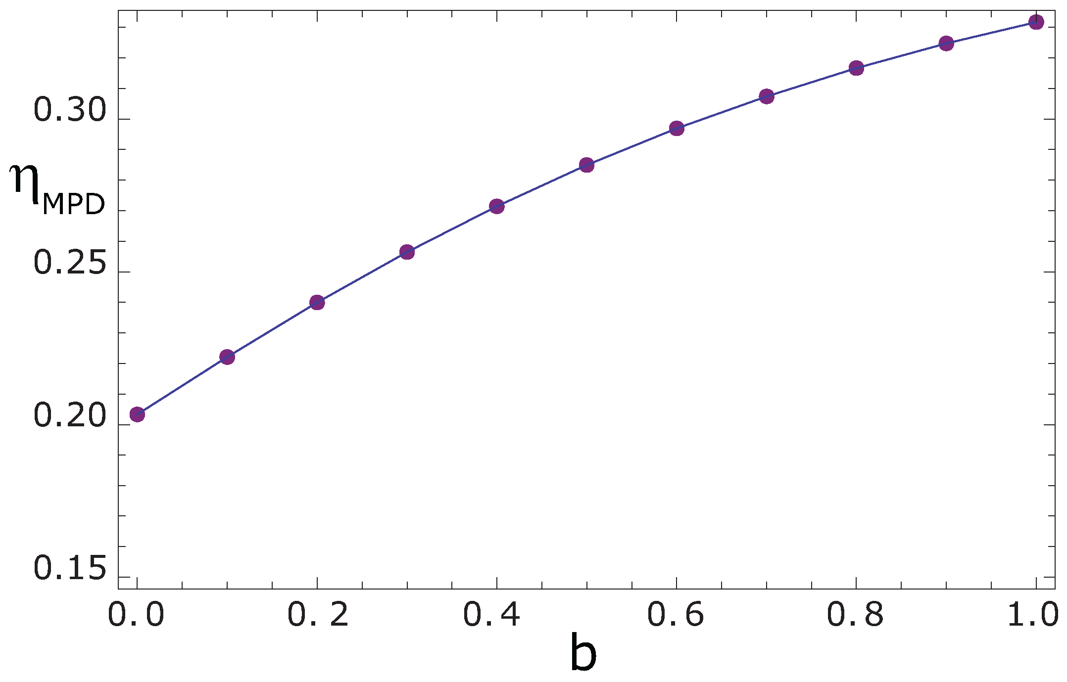
In this case we used $b=0.5$, because it represents the optimal value that maximizes the power density efficiency [35]. However, the effect of the conductance allocation parameter b at maximum power density obtained by means of the variational procedure is presented in Figure 3. It indicates, as Sahin stated, that as $b\to 0$, ${\eta }_{MPD}$ approaches to $1-\sqrt{\tau }$ and, for $b\to 1$, the efficiency ${\eta }_{MPD}$ increases to an upper limit depending on $\tau (=T_L/T_H)$. This result is similar to those obtained by Sahin [35] and De Vos [37] where they considered the engine size as an interesting parameter of study.

Figure 3. Effect of the conductance allocation parameter b on the efficiency at maximum power density.

Figure 3. Effect of the conductance allocation parameter b on the efficiency at maximum power density.

it can be noticed that under the maximum power density criterion, the efficiency for the Müser Stefan–Boltzmann engine is higher than in the ecological case or in the maximum power case, as many authors have pointed out [8,35].

5. Concluding Remarks

As far as is known, when dealing with optimization problems to obtain the efficiency for thermal engines in the context of the Finite Time Thermodynamics (FTT), it is not usual to use variational procedures for this purpose. In a previous work [24], Ares de Parga et al. showed that it was possible to use the variational methods to obtain the same results for the efficiency that the classical methods gave. Taking into account the former, the present work uses a simple variational procedure for obtaining the efficiency of an endoreversible CA Finite Time cycle of three different optimization criteria, namely

(a) the maximum power regime; (b) the ecological function criterion and (c) the maximum power density. All the analysis was made by means of a nonlinear heat transfer law (The Stefan–Boltzmann law), which is considered to represent the heat exchanges between reservoirs and working substance taking into account only radiative contributions.

The variational procedure allows obtaining two algebraic equations of fifth order for the temperatures of the isothermal processes for the maximum power and the ecological cases respectively. For the maximum power density case, an algebraic equation of eighth order was obtained. However, due to the order of the equations, it was not possible to obtain analytical solutions. To prove the validity of our results, we used the Müser engine, which has a main characteristic of perfect thermal contact with the surroundings. With this restriction, the results made by other authors, in particular those reported by De Vos [26], were produced with respect to the engine efficiency in the maximum power regime.

Due to the algebraic complexity of the solutions, there are no results for the ecological function regime and maximum power density with the characteristics mentioned before. In this work, interesting results for the maximum power density cases are presented.

For the nonlinear heat transfer law, the verification of the semi-sum property for the ecological case is of special interest. For the ecological regime, the efficiency was ${\eta }_E=0.2597$, which is higher than the maximum power efficiency ${\eta }_{MP}=0.2029$, for the limit case of the Müser engine. This reinforces the idea that the ecological function criterion is more efficient than the maximum power regime.

However, looking at the maximum power density, the efficiency ${\eta }_{MDP}=0.2849$ is higher even than the ecological regime, for the interval of $b\ge 0.4$, as many other authors have pointed out [35].

For the Müser engine, the optimum efficiencies for the power output and the ecological function could be considered as non-symmetric systems [33].