Capacity Bounds and Mapping Design for Binary Symmetric Relay Channels

Abstract

Capacity bounds for a three-node binary symmetric relay channel with orthogonal components at the destination are studied. The cut-set upper bound and the rates achievable using decode-and-forward (DF), partial DF and compress-and-forward (CF) relaying are first evaluated. Then relaying strategies with finite memory-length are considered. An efficient algorithm for optimizing the relay functions is presented. The Boolean Fourier transform is then employed to unveil the structure of the optimized mappings. Interestingly, the optimized relay functions exhibit a simple structure. Numerical results illustrate that the rates achieved using the optimized low-dimensional functions are either comparable to those achieved by CF or superior to those achieved by DF relaying. In particular, the optimized low-dimensional relaying scheme can improve on DF relaying when the quality of the source-relay link is worse than or comparable to that of other links.

1. Introduction

In this paper we consider a relay network consisting of a source, a relay, and a destination, as illustrated in Figure 1. This channel is considered in [1,2]. The communication task is to reproduce the transmitted message M, uniformly chosen from the set $\mathcal{M}=\{1,2,\dots ,2^{nR}\}$, at the destination such that the probability of error is arbitrarily small. The transmission of a message consumes n channel uses. We desire to quantify the supremum of the set of rates, R, for which the average message error probability at the destination can be made to approach zero as the number of channel uses n goes to infinity. This number is the capacity, C, in the communication between the source and destination. The channel capacity for the general relay channel is still an open problem.

Figure 1. Three-node relay network.

Figure 1. Three-node relay network.

One special case of the general relay channel is the Gaussian relay channel, which is studied, e.g., in [2,3,4,5,6,7,8,9]. In this paper, however, we focus on a relay network in which each link is a binary symmetric channel. Some instances of the binary symmetric relay channel (BSRC) are considered in [10,11,12,13,14]. The work of [10,11] considers BSRCs with correlated noises and [12,13] focuses on the detect-and-forward protocol for multi-hop relaying and the relay channel, respectively. In this paper, we consider a model that is also studied in an independent work [14]. We study decode-and-forward (DF), partial decode-and-forward (PDF), compress-and-forward (CF) and general finite-memory relay mappings. One of our main contributions is to propose a general structure for finite dimensional relaying. We show that one can improve on the result presented in [14] and illustrate that it is possible to approach the capacity upper bound for some cases by using the proposed low-dimensional mappings. Interestingly we recover the lower bound in [14] by a simple one-dimensional mapping at the relay. We also illustrate that one can obtain higher reliable rates by employing optimized relaying functions with larger memories. The rate obtained via optimized finite-length mappings can be superior to those achieved by DF protocol in some cases and are comparable to those achieved by CF protocol in general.

The remaining part of the paper is organized as follows. In Section 2, we present the three-node BSRC with orthogonal components at the destination. Section 3 derives capacity bounds for the BSRC when the relay is assumed to have infinite memory. Section 4 investigates capacity bounds for the BSRC when the relay is assumed to have a finite memory. We present an algorithm to optimize the relay mapping in Section 4. In Section 5 we compare the achievable rates as a function of memory length. Finally, Section 6 concludes the paper.

Notation: We use the following notation for brevity.

• ${\mathbb{GF}}_b$ denotes the binary Galois filed, i.e., $\{0,1\}$.
• ${\mathbb{GF}}_b^k$ denotes the k-dimensional binary Galois filed, i.e., ${\{0,1\}}^k$.
• ${\mathbb{H}}_{\text{b}}\left(ϵ\right):=-ϵlog\left(ϵ\right)-(1-ϵ)log(1-ϵ)$ denotes binary entropy function where $ϵ\in [0,1]$.
• ${\mathbb{D}}_{\text{H}}(x_1^k,y_1^k)$ denotes the Hamming distance between the two binary sequences of length k.
• The operation * is defined as ${ϵ}_1*{ϵ}_2:={ϵ}_1+{ϵ}_2-2{ϵ}_1{ϵ}_2$.
• We denote that the binary random variable Z has a Bernoulli distribution by $Z\sim \text{Ber}\left(ϵ\right)$ where $\text{Pr}(Z=1)=ϵ$ and $\text{Pr}(Z=0)=1-ϵ$.
• We denote the binary Kronecker delta function by ${\delta }_b\left(x\right)$, where ${\delta }_b\left(0\right)=1$ and ${\delta }_b\left(1\right)=0$ for $x\in {\mathbb{GF}}_b$.

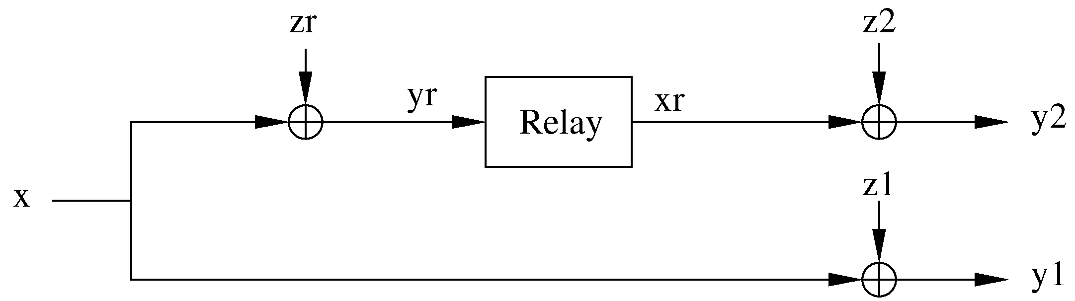
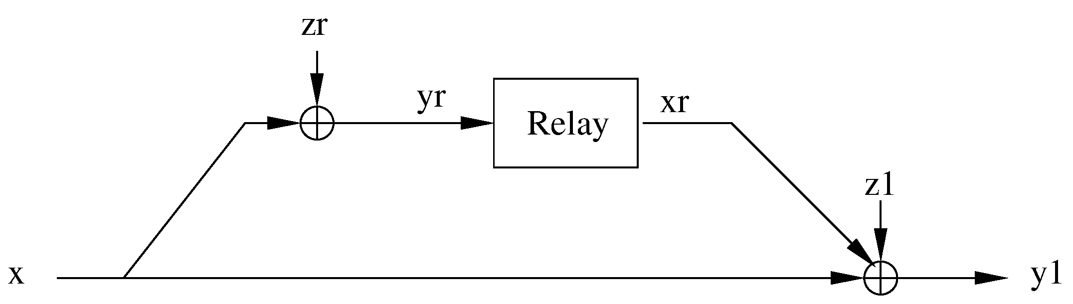
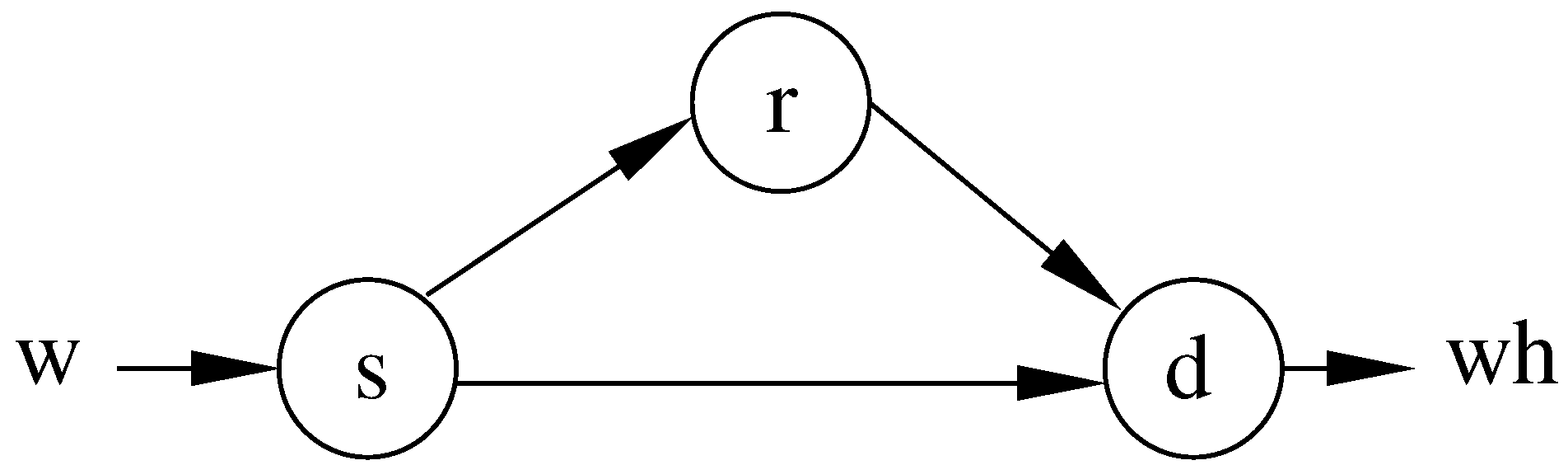
2. Binary Symmetric Relay Channel

In this section, we introduce the channel model that we consider in the paper. Figure 2 shows a BSRC consisting of three nodes: a source, a relay and a destination. In this model, we however assume that received signals at the destination are orthogonal. That is, the signals transmitted from the source and the relay do not interfere with each other. We further assume that all links are corrupted with modulo-sum noises distributed according to the Bernoulli distribution and all quantities are binary; i.e., $X,X_r,Y_1,Y_2,Y_r\in \{0,1\}$.

The received signal at the relay $Y_r$ is given by

$$Y_r=X\oplus Z_r$$

(1)

where X is the transmitted symbol from the source and $Z_r\sim \text{Ber}\left({ϵ}_r\right)$ is the additive Bernoulli noise. (The Bernoulli noise models for example the conventional communication set-up using BPSK modulation followed by a hard decision (see also [14]).) The received signal from the source at the destination $Y_1$ is given by

$$\begin{array}{ccc}\hfill Y_1& =& X\oplus Z_1\hfill \end{array}$$

(2)

where $Z_1\sim \text{Ber}\left({ϵ}_1\right)$ is the additive Bernoulli noise. Similarly, the received signal from the relay at the destination $Y_2$ is given by

$$\begin{array}{ccc}\hfill Y_2& =& X_r\oplus Z_2\hfill \end{array}$$

(3)

where $X_r$ is the transmitted symbol from the relay and $Z_2\sim \text{Ber}\left({ϵ}_2\right)$ is the additive Bernoulli noise. We assume that the random variables $Z_r$, $Z_1$, and $Z_2$ are mutually independent. Note that the addition in Equations (1)–(3) is done in $\mathbb{GF}\left(2\right)$.

Remark 1. Figure 3 shows a BSRC with non-orthogonal reception at the destination. The received signal at the destination is given by

$$\begin{array}{ccc}\hfill Y& =& X\oplus X_r\oplus Z\hfill \end{array}$$

(4)

where X and $X_r$ respectively denote the symbols transmitted by the source and the relay. The random variable $Z\sim \text{Ber}\left(ϵ\right)$ is the additive Bernoulli noise and is independent of $Z_r$. The capacity of this channel is

$$C_{no}=1-{\mathbb{H}}_{\text{b}}\left(ϵ\right)$$

(5)

By setting $X_r=0$, we have $Y=X\oplus Z$. Then the achievability follows since ${max}_{p\left(x\right)}I(X;Y|X_r=0)=C_{no}$. The converse follows from the cut-set bound. Invoking the multiple access bound, we have

$$\begin{array}{ccc}\hfill C& \le & I(X,X_r;Y)\hfill \\ & =& H\left(Y\right)-H\left(Y\right|X,X_r)\hfill \\ & =& H\left(Y\right)-H\left(Z\right)\hfill \\ & \le & 1-{\mathbb{H}}_{\text{b}}\left(ϵ\right)\hfill \end{array}$$

(6)

In the sequel, we present various capacity bounds for the orthogonal BSRC.

Figure 2. Orthogonal Binary Symmetric Relay Channel.

Figure 2. Orthogonal Binary Symmetric Relay Channel.

Figure 3. Non-Orthogonal Binary Symmetric Relay Channel.

Figure 3. Non-Orthogonal Binary Symmetric Relay Channel.

3. Capacity Bounds for the Orthogonal BSRC: Infinite Memory Relay Case

In this section, we consider the cut-set upper bound and three lower bounds on the capacity: DF, PDF and CF. These three bounds are evaluated based on the results in [2] for the general relay channel where the relay has infinite memory and unlimited processing capability.

Proposition 1 (cutset bound). For the relay channel in Figure 2, the capacity is upper bounded by

$$\begin{array}{ccc}\hfill R_{UB}& =& min\left\{1+{\mathbb{H}}_{\text{b}}({ϵ}_1*{ϵ}_r)-{\mathbb{H}}_{\text{b}}\left({ϵ}_1\right)-{\mathbb{H}}_{\text{b}}\left({ϵ}_r\right),2-{\mathbb{H}}_{\text{b}}\left({ϵ}_1\right)-{\mathbb{H}}_{\text{b}}\left({ϵ}_2\right)\right\}.\hfill \end{array}$$

(7)

Proof. See Appendix A and also [14].  ☐

Proposition 2 (DF lower bound). For the relay channel in Figure 2, the capacity is lower bounded by

$$\begin{array}{ccc}\hfill R_{DF}=max\{1-{\mathbb{H}}_{\text{b}}\left({ϵ}_1\right)& ,& min\{1-{\mathbb{H}}_{\text{b}}\left({ϵ}_r\right),2-{\mathbb{H}}_{\text{b}}\left({ϵ}_1\right)-{\mathbb{H}}_{\text{b}}\left({ϵ}_2\right)\}\}\hfill \end{array}$$

(8)

where the bound is achieved using the block Markov encoding scheme in [2] (known as DF relaying) and the only-direct-transmission (i.e., when the relay is off).

Proof. See Appendix B. ☐

Note that in Equation (8), we take the maximum of the rates achieved using the conventional DF [2] and the only-direct-link transmission. In some cases it is possible to improve on DF by using PDF at the relay. That is, the relay only decodes a part of the transmitted message. The achievable rate of PDF is given by

$$\begin{array}{ccc}\hfill R_{PDF}& =& \underset{p(u,x,x_r)}{max}min\{I(X,X_r;Y_1,Y_2),I(U;Y_r|X_r)+I(X;Y_1,Y_2|X_r,U)\}\hfill \end{array}$$

(9)

where U denotes the part of the transmitted message that the relay decodes. (See Theorem 7 in [2] and also [15].)

Proposition 3 (PDF lower bound). For the relay channel in Figure 2, generalized block Markov encoding attains the same rate as the modified DF given in Equation (8).

Proof. See Appendix C.  ☐

Corollary 1. DF is an optimal relaying strategy if ${\mathbb{H}}_{\text{b}}\left({ϵ}_1\right)+{\mathbb{H}}_{\text{b}}\left({ϵ}_2\right)-{\mathbb{H}}_{\text{b}}\left({ϵ}_r\right)\ge 1$.

Proof. The proof follows from Propositions 2 and 1.  ☐

Proposition 4 (CF lower bound). For the relay channel in Figure 2, the capacity is lower bounded by

$$R_{CF}=\left\{\begin{array}{cc}1+{\mathbb{H}}_{\text{b}}({ϵ}_1*{ϵ}_r*{ϵ}_q)-{\mathbb{H}}_{\text{b}}({ϵ}_r*{ϵ}_q)-{\mathbb{H}}_{\text{b}}\left({ϵ}_1\right),\hfill & \mathit{if}1<{\mathbb{H}}_{\text{b}}\left({ϵ}_2\right)+{\mathbb{H}}_{\text{b}}({ϵ}_1*{ϵ}_r)\hfill \\ \\ 1+{\mathbb{H}}_{\text{b}}({ϵ}_1*{ϵ}_r)-{\mathbb{H}}_{\text{b}}\left({ϵ}_r\right)-{\mathbb{H}}_{\text{b}}\left({ϵ}_1\right),\hfill & \mathit{if}1\ge {\mathbb{H}}_{\text{b}}\left({ϵ}_2\right)+{\mathbb{H}}_{\text{b}}({ϵ}_1*{ϵ}_r)\hfill \end{array}\right.$$

(10)

where ${ϵ}_q$ satisfies

$${\mathbb{H}}_{\text{b}}({ϵ}_1*{ϵ}_r*{ϵ}_q)-{\mathbb{H}}_{\text{b}}\left({ϵ}_q\right)+{\mathbb{H}}_{\text{b}}\left({ϵ}_2\right)=1$$

(11)

Proof. See Appendix D.  ☐

The bound in Equation (10) is achieved using the side-information encoding scheme in [2], known as CF relaying.

Corollary 2. CF is an optimal relaying strategy if ${\mathbb{H}}_{\text{b}}({ϵ}_1*{ϵ}_r)+{\mathbb{H}}_{\text{b}}\left({ϵ}_2\right)\le 1$.

Proof. The proof follows from Propositions 4 and 1.  ☐

Figure 4. Optimal regions for ${ϵ}_2=0.05$.

Figure 4. Optimal regions for ${ϵ}_2=0.05$.

Figure 4 and Figure 5 show optimal regions in the plane [0, 1]×[0, 1] for ϵ₂ set to 0.05 and 0.2, respectively. One can see that for some parameters of ϵ_r and ϵ₁, CF or DF is optimal.

From Figure 4 and Figure 5, we see that DF is optimal when ϵ_r is small and ϵ₁ is close to 0.5. When ϵ₁ = 0.5, the BSRC simplifies to a two-hop channel for which DF is capacity achieving. However, DF is also optimal when the relay is relatively strong compared with the direct link.

From Figure 4 and Figure 5, we similarly see that CF is optimal at the corner of the plane, i.e., when ϵ₁ and ϵ_r are small. As ϵ₂ increases, the area of the region for which CF is optimal shrinks. This is due to the fact that small value of ϵ₂ allows the relay to use higher rate to describe the received signal to destination. Small value of ϵ₁ means the destination has better side-information in order to decode the reproduction sequence generated at the relay, and small value of ϵ_r means that the relay receives a less-noisy sequence on average that makes compression of the “true” signal easier.

Figure 5. Optimal regions for ${ϵ}_2=0.2$.

Figure 5. Optimal regions for ${ϵ}_2=0.2$.

4. Capacity Bounds for the Orthogonal BSRC: Finite Memory Relay Case

We next consider the case when the relay has a finite memory length. For the Gaussian relay channel, optimized memoryless relaying is investigated in [16,17,18,19]. Here we consider higher-dimension mappings for the BSRC.

If the relay has a storage memory of k bits, it can process the last $k-1$ and the presently received symbol to generate k new symbols using k possibly different k-dimensional functions. This results in a low-complexity relaying protocol suitable for delay-sensitive or inexpensive applications. In the following, we denote the relay functions by

$$\begin{array}{c}{f}_i:{\mathbb{GF}}_b^k⟼{\mathbb{GF}}_b\hfill \\ x_{r,i}=f_i(y_{r,1},\dots ,y_{r,k})\hfill \end{array}$$

(12)

for $i\in \{1,2,\dots ,k\}$. Note that we here consider the whole sub-block of k symbols to generate k new symbols to be transmitted to the destination. This is different from the classical definition with strictly causal relaying. We are allowed to do this, without any particular condition in signal reception at the relay, since the relay has an orthogonal link to the destination.

4.1. Achievable Rate

For a given set of relay functions ${\left\{f_i\right\}}_{i=1}^k$, the channel is parameterized by the pmf $p\left(\mathbf{y}\right|\mathbf{x})$, by defining $\mathbf{y}\equiv (y_{1,1}^k,y_{2,1}^k)$ and $\mathbf{x}\equiv x_1^k$, where

$$\begin{array}{ccc}\hfill p\left(\mathbf{y}|\mathbf{x}\right)& :=& p\left(y_{1,1}^k,y_{2,1}^k|x_1^k\right)\hfill \\ & =& \sum _{y_{r,1}^k\in {\mathbb{GF}}_b^k}p\left(y_{1,1}^k,y_{2,1}^k|y_{r,1}^k,x_1^k\right)p\left(y_{r,1}^k|x_1^k\right)\hfill \\ & =& \sum _{y_{r,1}^k\in {\mathbb{GF}}_b^k}p\left(y_{1,1}^k|x_1^k\right)p\left(y_{2,1}^k|y_{r,1}^k\right)p\left(y_{r,1}^k|x_1^k\right)\hfill \\ & =& \sum _{y_{r,1}^k\in {\mathbb{GF}}_b^k}\prod _{i=1}^{k}p\left(y_{1,i}|x_i\right)p\left(y_{r,i}|x_i\right)p(y_{2,i}|f_i(y_{r,1}^k))\hfill \\ & =& \sum _{y_{r,1}^k\in {\mathbb{GF}}_b^k}\prod _{i=1}^k\left[(1-{ϵ}_1){\delta }_b\left(y_{1,i}\oplus x_i\right)+{ϵ}_1{\delta }_b\left(y_{1,i}\oplus x_i\oplus 1\right)\right]\times \hfill \\ & & \left[(1-{ϵ}_r){\delta }_b\left(y_{r,i}\oplus x_i\right)+{ϵ}_r{\delta }_b\left(y_{r,i}\oplus x_i\oplus 1\right)\right]\times \hfill \\ & & \left[(1-{ϵ}_2){\delta }_b(y_{2,i}\oplus f_i(y_{r,1}^k))+{ϵ}_2{\delta }_b(y_{2,i}\oplus f_i(y_{r,1}^k)\oplus 1)\right]\hfill \end{array}$$

(13)

Now one can apply the standard random coding argument for the equivalent discrete memoryless point-to-point communication link with the input $\mathbf{x}$ and the output $\mathbf{y}$ whose relation is governed by the pmf $p\left(\mathbf{y}|\mathbf{x}\right)$ as follows. Generate $2^{\left(nk\right)C_k}$ i.i.d. codewords where each has length $kn$ and each k subsequent symbols in every codeword is distributed according to $p\left(x_1^k\right)$ (i.e., $p\left(x_1^{kn}\right)={\prod }_{i=1}^{n}p\left(x_1^k\right)$). Thus, the achievable rate using the finite memory relay is given by

$$C_k=\underset{{\left\{f_i\right\}}_{i=1}^k,p\left(x_1^k\right)}{sup}\frac{1}{k}I(X_1^k;Y_{1,1}^k,Y_{2,1}^k)$$

(14)

where the supremum is taken over the set of Boolean functions ${\left\{f_i\right\}}_{i=1}^k$ and the joint pmf $p\left(x_1^k\right)$ of k symbols at the source. Since the channel is used k times, the mutual information in Equation (14) is divided by k (see also [1,4]).

Achievable Rate for $k=1$: The simplest case is the memoryless relay in which the relay just transmits the received noisy bit to the destination without any further processing. That is $x_{r,i}=y_{r,i}$ for $1\le i\le n$. For this relay function, the optimal input distribution is $X\sim \text{Ber}\left(\frac{1}{2}\right)$.

Proposition 5. For the relay channel in Figure 2, the rate

$$C_1=1+{\mathbb{H}}_{\text{b}}({ϵ}_1*{ϵ}_r*{ϵ}_2)-{\mathbb{H}}_{\text{b}}({ϵ}_r*{ϵ}_2)-{\mathbb{H}}_{\text{b}}\left({ϵ}_1\right)$$

(15)

is achievable.

Proof. See Appendix E.  ☐

We note that the rate $C_1$ is also derived in [14] via a suboptimal evaluation of the CF lower bound. However, here we arrive at this rate using a one-dimensional mapping without any need for a compression codebook at the relay.

Computation of $C_k$ for $k\ge 2$ is a cumbersome task. Nevertheless, there is no unique set of relay functions that is optimal for all channel parameters ${ϵ}_r$, ${ϵ}_1$, ${ϵ}_2$. To see this, consider the case with ${ϵ}_2=0$. For this case, the simple strategy with $k=1$ used in Proposition 5 is optimal. However, this relay function is not necessarily optimal for cases with ${ϵ}_2\ne 0$ since one can potentially provide error protection on the relay-destination link by utilizing functions with higher dimensions.

4.2. Mapping Optimization for an Arbitrary k

In the following, we confine the pmf at the source to be $p\left(x_1^k\right)={\prod }_{i=1}^{k}p\left(x\right)$, and $p\left(x\right)=\frac{1}{2}{\delta }_b\left(x\right)+\frac{1}{2}{\delta }_b(x\oplus 1)$, i.e., $X\sim \text{Ber}\left(\frac{1}{2}\right)$.

Lemma 1. The mutual information given in Equation (14) can be written as

$$\begin{array}{ccc}\hfill \frac{1}{k}I(X_1^k;Y_{1,1}^k,Y_{2,1}^k)& =& 1-{\mathbb{H}}_{\text{b}}\left({ϵ}_1\right)-\frac{1}{k}\mathbb{E}\left[log(p(y_{2,1}^k|y_{1,1}^k))\right]+\frac{1}{k}\mathbb{E}\left[log(p(y_{2,1}^k|x_1^k))\right]\hfill \end{array}$$

(16)

where

$$\begin{array}{ccc}& & p\left(y_{2,1}^k\right|x_1^k)={(1-{ϵ}_2)}^k{(1-{ϵ}_r)}^k\sum _{y_{r,1}^k\in {\mathbb{GF}}_b^k}{\left(\frac{{ϵ}_2}{1-{ϵ}_2}\right)}^{{\mathbb{D}}_{\text{H}}(y_{2,1}^k,f\left(y_{r,1}^k\right))}{\left(\frac{{ϵ}_r}{1-{ϵ}_r}\right)}^{{\mathbb{D}}_{\text{H}}(y_{r,1}^k,x_1^k)}\hfill \end{array}$$

(17)

and

$$\begin{array}{cc}\hfill p& \left(y_{2,1}^k\right|y_{1,1}^k)=\hfill \end{array}$$

$$\begin{array}{cc}& {(1-{ϵ}_1)}^k{(1-{ϵ}_2)}^k{(1-{ϵ}_r)}^k\sum _{y_{r1}^k\in {\mathbb{GF}}_b^k}{\left(\frac{{ϵ}_2}{1-{ϵ}_2}\right)}^{{\mathbb{D}}_{\text{H}}(y_{2,1}^k,f\left(y_{r,1}^k\right))}\sum _{x_1^k\in {\mathbb{GF}}_b^k}{\left(\frac{{ϵ}_r}{1-{ϵ}_r}\right)}^{{\mathbb{D}}_{\text{H}}(y_{r,1}^k,x_1^k)}{\left(\frac{{ϵ}_1}{1-{ϵ}_1}\right)}^{{\mathbb{D}}_{\text{H}}(y_{1,1}^k,x_1^k)}.\hfill \end{array}$$

(18)

Proof. See Appendix F. ☐

To compute the rate in Equation (14), one needs to select the best functions among $2^{k{2}^k}$ possible choices, which has a exponential complexity. (For $k=4$, there are approximately $1.8\times {10}^{19}$ possible functions.) In order to cope with the complexity, we implement an efficient hill-climbing search algorithm as follows. For a given k, we first initialize the relay functions with a random mapping and compute the rate using Lemma 1. Then we randomly select one function and one corresponding dimension, and flip the mapping and recompute the rate. If the new mapping provides a higher rate, we accept the change. Otherwise we repeat the process until the mapping converges. Since the algorithm by construction may terminate in a local optimum, we repeat the whole algorithm with different initializations and pick the mapping that attains the highest rate.

One example of the optimized mapping for $k=4$ when ${ϵ}_1={ϵ}_2={ϵ}_r=0.01$ is

$$\begin{array}{c}\hfill F=\left[\begin{array}{cccccccccccccccc}0& 0& 1& 1& 1& 1& 0& 0& 1& 1& 0& 0& 0& 0& 1& 1\\ 1& 0& 0& 1& 0& 1& 1& 0& 1& 0& 0& 1& 0& 1& 1& 0\\ 1& 0& 0& 1& 1& 0& 0& 1& 0& 1& 1& 0& 0& 1& 1& 0\\ 1& 0& 1& 0& 0& 1& 0& 1& 0& 1& 0& 1& 1& 0& 1& 0\end{array}\right].\end{array}$$

Here $F_{ij}$ denotes the output of the relay along the ith dimension for the jth input configuration (we have $1\le i\le 4$ and $1\le j\le 2^4$). The relay for a given combination of the received bits finds the decimal representation and transmits the bits in the column given by the decimal representation plus one. For example, for the received string 0000, the relay transmits the bits in the first column, i.e., 0111. By studying the matrix F, we can get some insight into the underlying structure of the mapping. Finding an efficient structure at the relay simplifies the design and the implementation of relaying. We employ the Fourier transform to accomplish this task. Our use of the binary Fourier (or Hadamard) transform is related to how it was used in, e.g., [20,21], to analyze the performance of quantizers over noisy channels.

4.3. Fourier Spectrum of the Optimized Mappings

In order to define the Fourier transform, we need an orthonormal basis [22]. Consider the following set of functions

$$\begin{array}{c}{\mathcal{X}}_S\left(\mathbf{x}\right):{\{-1,+1\}}^k⟼\{-1,+1\}\hfill \\ {\mathcal{X}}_S\left(\mathbf{x}\right)=\prod _{i\in S}{x}_i\hfill \end{array}$$

(19)

where $S\subseteq \{1,2,\cdots ,k\}$. Then, any function $f:{\{0,1\}}^k\to \{0,1\}$ can uniquely be represented as (We use the one-to-one mapping $0⟺+1$ and $1⟺-1$.)

$$\begin{array}{c}\hfill f=\sum _{S\subseteq \{1,2,\cdots ,k\}}\widehat{f}\left(S\right){\mathcal{X}}_S\end{array}$$

(20)

where $\widehat{f}\left(S\right)$ is the Fourier coefficient of f and is given by

$$\begin{array}{ccc}\hfill \widehat{f}\left(S\right)& =& \langle f,{\mathcal{X}}_S\rangle =\frac{1}{2^k}\sum _{\mathbf{x}\in {\{+1,-1\}}^k}f\left(\mathbf{x}\right){\mathcal{X}}_S\left(\mathbf{x}\right)\hfill \\ & =& \mathbb{E}\left[f·{\mathcal{X}}_S\right]\hfill \end{array}$$

(21)

The expectation in Equation (21) is taken uniformly over $\mathbf{x}\in {\{+1,-1\}}^k$. Note that the Fourier expansion of f can potentially have up to $2^k$ terms. As an example consider the following randomly chosen function.

x3	x2	x1		f
+ 1	+ 1	+ 1		+ 1
+ 1	+ 1	− 1		+ 1
+ 1	− 1	+ 1		− 1
+ 1	− 1	− 1		− 1
− 1	+ 1	+ 1		− 1
− 1	+ 1	− 1		+ 1
− 1	− 1	+ 1		+ 1
− 1	− 1	− 1		+ 1

This function can be expanded as

$$\begin{array}{ccc}\hfill f(x_1,x_2,x_3)& =& \frac{1}{4}-\frac{1}{4}{x}_1+\frac{1}{4}{x}_2-\frac{1}{4}{x}_3-\frac{1}{4}{x}_1{x}_2+\frac{1}{4}{x}_1{x}_3+\frac{3}{4}{x}_2{x}_3+\frac{1}{4}{x}_1{x}_2{x}_3\hfill \end{array}$$

(22)

That is, the Fourier spectrum has eight terms and the function is not linear. In general, we would like a sparse Fourier spectrum for efficient implementation. (Sparsity of mappings allows to realize them with much fewer multiplications and additions. This can be also compared to codes with low-density generator/parity matrices that allow simpler encoding and decoding in general.)

Table 1 presents the Fourier expansion of optimized relay functions for $k=2,3,4,6$ when ${ϵ}_1={ϵ}_2={ϵ}_r=0.01$. Interestingly, we see that that the Fourier expansion of the optimized functions is indeed sparse. Using the results in Table 1, we can rewrite the functions in the following form

$$\begin{array}{ccc}& & f:{\{0,1\}}^k⟼{\{0,1\}}^k\hfill \\ & & {\mathbf{x}}_r=A_k{\mathbf{y}}_r+b_k\hfill \end{array}$$

(23)

where ${\mathbf{x}}_r={[x_{r,1},\dots ,x_{r,k}]}^T$ and ${\mathbf{y}}_r={[y_{r,1},\dots ,y_{r,k}]}^T$, and $A_k\in {\{0,1\}}^{[k\times k]}$ and $b_k\in {\{0,1\}}^{[k\times 1]}$. For example for $k=6$, we have

$$\begin{array}{ccc}& & A_6=\left[\begin{array}{cccccc}0& 1& 1& 0& 1& 0\\ 1& 0& 1& 1& 0& 1\\ 0& 1& 0& 1& 1& 0\\ 1& 1& 1& 1& 0& 0\\ 1& 0& 0& 0& 1& 1\\ 0& 1& 1& 1& 0& 1\end{array}\right],b_6=\left[\begin{array}{c}0\\ 1\\ 1\\ 1\\ 0\\ 1\end{array}\right]\hfill \end{array}$$

Note that the mapping given in Equation (23) is not linear in the binary field, when $b_k\ne \mathbf{0}$. However, the linear mapping ${\mathbf{x}}_r=A_k{\mathbf{y}}_r$ gives the same performance as ${\mathbf{x}}_r=A_k{\mathbf{y}}_r+b_k$. In other words the bias term $b_k$ does not improve the rate. This essentially follows from the data processing inequality. Therefore, the underlying relay functions define a linear code of rate one on the noisy received bits at the relay. Additionally, the code used at the relay performs joint source–channel coding, it therefore should be good for both source and channel coding.

Table 1. Fourier expansion of the optimized relay functions for the orthogonal BSRC with ${ϵ}_1={ϵ}_2={ϵ}_r=0.01.$

$k=2$	$\begin{array}{c}{f}_1\left(y_{r1}^k\right)=y_{r1}\hfill \\ f_2\left(y_{r1}^k\right)=y_{r2}{y}_{r1}\hfill \end{array}$
$k=3$	$\begin{array}{c}{f}_1\left(y_{r1}^k\right)=y_{r3}{y}_{r2}{y}_{r1}\hfill \\ f_2\left(y_{r1}^k\right)=-y_{r3}{y}_{r1}\hfill \\ f_3\left(y_{r1}^k\right)=y_{r3}{y}_{r2}\hfill \end{array}$
$k=4$	$\begin{array}{c}{f}_1\left(y_{r1}^k\right)=-y_{r4}{y}_{r3}{y}_{r1}\hfill \\ f_2\left(y_{r1}^k\right)=-y_{r4}{y}_{r2}{y}_{r1}\hfill \\ f_3\left(y_{r1}^k\right)=-y_{r3}{y}_{r2}{y}_{r1}\hfill \\ f_4\left(y_{r1}^k\right)=y_{r4}{y}_{r3}{y}_{r2}\hfill \end{array}$
$k=6$	$\begin{array}{c}{f}_1\left(y_{r1}^k\right)=y_{r5}{y}_{r3}{y}_{r2}\hfill \\ f_2\left(y_{r1}^k\right)=-y_{r6}{y}_{r4}{y}_{r3}{y}_{r1}\hfill \\ f_3\left(y_{r1}^k\right)=-y_{r5}{y}_{r4}{y}_{r2}\hfill \\ f_4\left(y_{r1}^k\right)=-y_{r4}{y}_{r3}{y}_{r2}{y}_{r1}\hfill \\ f_5\left(y_{r1}^k\right)=y_{r6}{y}_{r5}{y}_{r1}\hfill \\ f_6\left(y_{r1}^k\right)=-y_{r6}{y}_{r4}{y}_{r3}{y}_{r2}\hfill \end{array}$

Table 1. Fourier expansion of the optimized relay functions for the orthogonal BSRC with ${ϵ}_1={ϵ}_2={ϵ}_r=0.01.$

$k=2$	$\begin{array}{c}{f}_1\left(y_{r1}^k\right)=y_{r1}\hfill \\ f_2\left(y_{r1}^k\right)=y_{r2}{y}_{r1}\hfill \end{array}$
$k=3$	$\begin{array}{c}{f}_1\left(y_{r1}^k\right)=y_{r3}{y}_{r2}{y}_{r1}\hfill \\ f_2\left(y_{r1}^k\right)=-y_{r3}{y}_{r1}\hfill \\ f_3\left(y_{r1}^k\right)=y_{r3}{y}_{r2}\hfill \end{array}$
$k=4$	$\begin{array}{c}{f}_1\left(y_{r1}^k\right)=-y_{r4}{y}_{r3}{y}_{r1}\hfill \\ f_2\left(y_{r1}^k\right)=-y_{r4}{y}_{r2}{y}_{r1}\hfill \\ f_3\left(y_{r1}^k\right)=-y_{r3}{y}_{r2}{y}_{r1}\hfill \\ f_4\left(y_{r1}^k\right)=y_{r4}{y}_{r3}{y}_{r2}\hfill \end{array}$
$k=6$	$\begin{array}{c}{f}_1\left(y_{r1}^k\right)=y_{r5}{y}_{r3}{y}_{r2}\hfill \\ f_2\left(y_{r1}^k\right)=-y_{r6}{y}_{r4}{y}_{r3}{y}_{r1}\hfill \\ f_3\left(y_{r1}^k\right)=-y_{r5}{y}_{r4}{y}_{r2}\hfill \\ f_4\left(y_{r1}^k\right)=-y_{r4}{y}_{r3}{y}_{r2}{y}_{r1}\hfill \\ f_5\left(y_{r1}^k\right)=y_{r6}{y}_{r5}{y}_{r1}\hfill \\ f_6\left(y_{r1}^k\right)=-y_{r6}{y}_{r4}{y}_{r3}{y}_{r2}\hfill \end{array}$

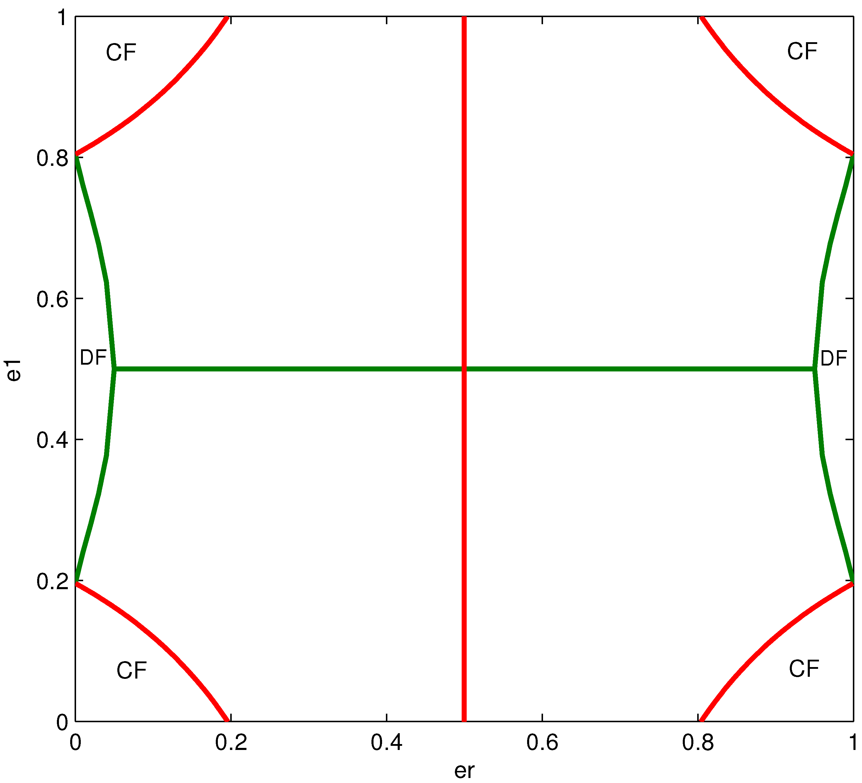
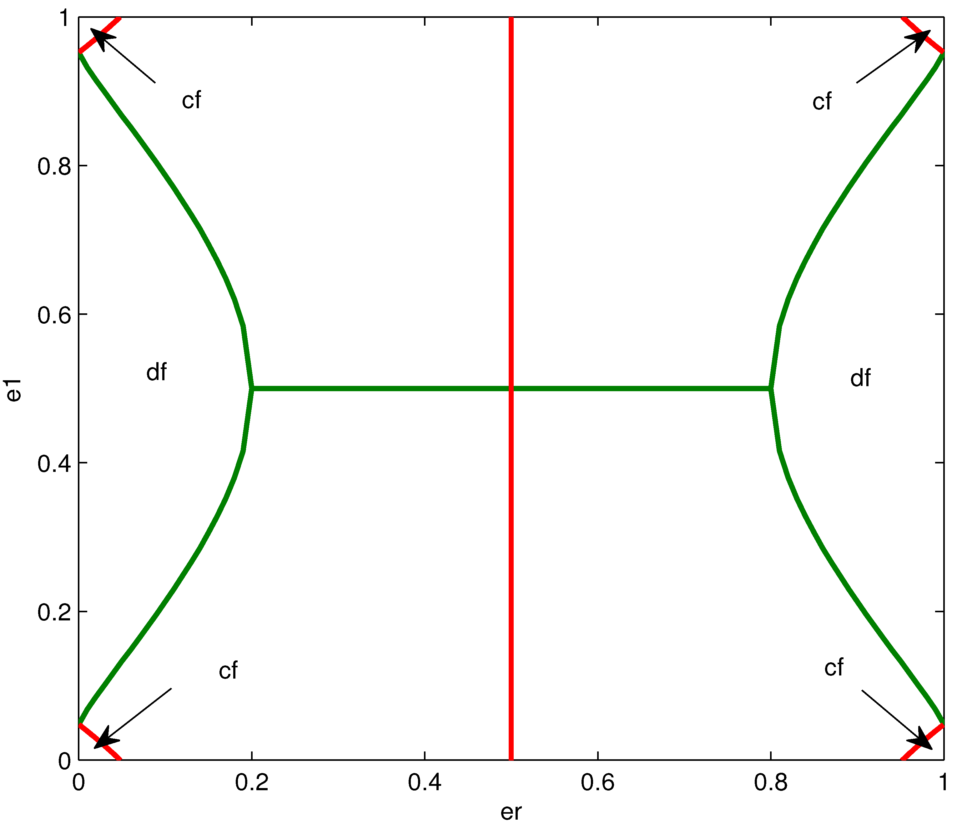
4.4. Effect of Channel Parameters on the Structure of the Optimized Mappings

In this section, we investigate the structure of the optimized mappings for different channel parameters. Our numerical search indicates that the linear mapping ${\mathbf{x}}_r=A_k{\mathbf{y}}_r$ is an efficient strategy among all classes of mappings for low-dimensional relaying. That is, the relay employs the binary matrix $A_k$ to generate the relay outputs using k received bits.

Table 2 shows the optimized generator matrices $A_k$ for various values of ${ϵ}_r$ when $k=6$, ${ϵ}_1={ϵ}_2=0.05$. In particular, for ${ϵ}_r=0.25$ the optimized generator matrix is the identity matrix, i.e., $A_6=I_6$. For this case, the relay is better off transmitting the received noisy bits without any further processing. However, as ${ϵ}_r$ decreases, the relay starts combining the received bits at the relay before transmitting. The number of ones in a row of the generator matrix indicates the number of inputs that the relay combines. The density of ones in the generator matrices $\rho :=\frac{\#\text{of}\text{ones}}{k^2}$ are also shown in Table 2. We see that as ${ϵ}_r$ decreases, ρ increases. That is, the relay starts to transmit combinations of more bits in one single channel use. This occurs because of two main reasons: firstly when ${ϵ}_r$ decreases the relay receives less noisy bits on average and secondly the destination has some partial knowledge of individual bits via the received signal from the source.

Table 3 shows the optimized generator matrices for various values of ${ϵ}_1$ when $k=6$, ${ϵ}_r=0.01$ and ${ϵ}_2=0.1$. We similarly see that as ${ϵ}_1$ decreases, ρ increases. This is due to the fact that when ${ϵ}_1$ decreases, the destination receives better descriptions of the transmitted bits via the source-destination link. The relay then forwards combinations of several incoming bits when the destination has access to more reliable side information.

Table 2. Optimized generator matrices as a function of ${ϵ}_r$ for $k=6$ and ${ϵ}_1={ϵ}_2=0.05$.

${ϵ}_r$	$0.25$	$0.1$	$0.05$	$0.01$	$0.001$	$0.0001$
$A_6$	$\left[\begin{array}{cccccc}1& 0& 0& 0& 0& 0\\ 0& 1& 0& 0& 0& 0\\ 0& 0& 1& 0& 0& 0\\ 0& 0& 0& 1& 0& 0\\ 0& 0& 0& 0& 1& 0\\ 0& 0& 0& 0& 0& 1\end{array}\right]$	$\left[\begin{array}{cccccc}0& 0& 1& 0& 0& 0\\ 0& 1& 0& 0& 0& 0\\ 0& 0& 0& 0& 0& 1\\ 0& 0& 0& 1& 1& 0\\ 1& 0& 0& 0& 1& 0\\ 1& 1& 1& 1& 1& 1\end{array}\right]$	$\left[\begin{array}{cccccc}1& 0& 0& 0& 1& 0\\ 1& 1& 1& 1& 0& 0\\ 1& 0& 1& 0& 0& 0\\ 1& 0& 0& 1& 1& 1\\ 0& 1& 0& 0& 1& 0\\ 0& 0& 0& 0& 1& 1\end{array}\right]$	$\left[\begin{array}{cccccc}1& 1& 0& 0& 0& 1\\ 0& 1& 0& 1& 1& 0\\ 0& 0& 1& 1& 1& 0\\ 1& 0& 1& 1& 0& 0\\ 1& 0& 1& 0& 1& 1\\ 0& 1& 1& 0& 1& 1\end{array}\right]$	$\left[\begin{array}{cccccc}1& 1& 1& 0& 0& 1\\ 0& 1& 1& 1& 0& 0\\ 0& 1& 1& 0& 1& 1\\ 1& 1& 0& 1& 1& 0\\ 1& 0& 0& 0& 1& 1\\ 1& 0& 1& 1& 1& 0\end{array}\right]$	$\left[\begin{array}{cccccc}1& 0& 0& 1& 0& 1\\ 0& 1& 0& 1& 0& 1\\ 1& 1& 1& 0& 0& 1\\ 1& 1& 1& 1& 1& 0\\ 1& 1& 0& 0& 1& 1\\ 0& 0& 1& 1& 1& 1\end{array}\right]$
ρ	0.1667	0.3611	0.4444	0.5556	0.6111	0.6389

Table 2. Optimized generator matrices as a function of ${ϵ}_r$ for $k=6$ and ${ϵ}_1={ϵ}_2=0.05$.

${ϵ}_r$	$0.25$	$0.1$	$0.05$	$0.01$	$0.001$	$0.0001$
$A_6$	$\left[\begin{array}{cccccc}1& 0& 0& 0& 0& 0\\ 0& 1& 0& 0& 0& 0\\ 0& 0& 1& 0& 0& 0\\ 0& 0& 0& 1& 0& 0\\ 0& 0& 0& 0& 1& 0\\ 0& 0& 0& 0& 0& 1\end{array}\right]$	$\left[\begin{array}{cccccc}0& 0& 1& 0& 0& 0\\ 0& 1& 0& 0& 0& 0\\ 0& 0& 0& 0& 0& 1\\ 0& 0& 0& 1& 1& 0\\ 1& 0& 0& 0& 1& 0\\ 1& 1& 1& 1& 1& 1\end{array}\right]$	$\left[\begin{array}{cccccc}1& 0& 0& 0& 1& 0\\ 1& 1& 1& 1& 0& 0\\ 1& 0& 1& 0& 0& 0\\ 1& 0& 0& 1& 1& 1\\ 0& 1& 0& 0& 1& 0\\ 0& 0& 0& 0& 1& 1\end{array}\right]$	$\left[\begin{array}{cccccc}1& 1& 0& 0& 0& 1\\ 0& 1& 0& 1& 1& 0\\ 0& 0& 1& 1& 1& 0\\ 1& 0& 1& 1& 0& 0\\ 1& 0& 1& 0& 1& 1\\ 0& 1& 1& 0& 1& 1\end{array}\right]$	$\left[\begin{array}{cccccc}1& 1& 1& 0& 0& 1\\ 0& 1& 1& 1& 0& 0\\ 0& 1& 1& 0& 1& 1\\ 1& 1& 0& 1& 1& 0\\ 1& 0& 0& 0& 1& 1\\ 1& 0& 1& 1& 1& 0\end{array}\right]$	$\left[\begin{array}{cccccc}1& 0& 0& 1& 0& 1\\ 0& 1& 0& 1& 0& 1\\ 1& 1& 1& 0& 0& 1\\ 1& 1& 1& 1& 1& 0\\ 1& 1& 0& 0& 1& 1\\ 0& 0& 1& 1& 1& 1\end{array}\right]$
ρ	0.1667	0.3611	0.4444	0.5556	0.6111	0.6389

Table 3. Optimized generator matrices as a function of ${ϵ}_1$ for $k=6$ and ${ϵ}_r=0.01$, ${ϵ}_2=0.1$.

${ϵ}_1$	$0.4$	$0.25$	$0.1$	$0.05$	$0.01$	$0.001$
$A_6$	$\left[\begin{array}{cccccc}1& 0& 0& 0& 0& 0\\ 0& 1& 0& 0& 0& 0\\ 0& 0& 1& 0& 0& 0\\ 0& 0& 0& 1& 0& 0\\ 0& 0& 0& 0& 1& 0\\ 0& 0& 0& 0& 0& 1\end{array}\right]$	$\left[\begin{array}{cccccc}0& 1& 1& 0& 0& 0\\ 1& 0& 0& 1& 0& 0\\ 0& 0& 1& 0& 0& 1\\ 1& 0& 0& 0& 0& 1\\ 0& 1& 0& 0& 1& 0\\ 0& 0& 0& 1& 1& 0\end{array}\right]$	$\left[\begin{array}{cccccc}1& 1& 0& 0& 1& 1\\ 0& 1& 0& 1& 0& 1\\ 0& 1& 1& 0& 1& 0\\ 1& 0& 0& 1& 1& 1\\ 1& 0& 1& 0& 1& 0\\ 1& 0& 1& 1& 0& 0\end{array}\right]$	$\left[\begin{array}{cccccc}1& 1& 1& 0& 1& 0\\ 1& 0& 1& 1& 0& 0\\ 1& 0& 1& 0& 1& 1\\ 0& 1& 1& 1& 1& 1\\ 1& 0& 0& 1& 1& 0\\ 1& 1& 0& 1& 0& 1\end{array}\right]$	$\left[\begin{array}{cccccc}1& 0& 1& 0& 1& 1\\ 1& 1& 0& 1& 0& 1\\ 0& 1& 0& 1& 1& 1\\ 1& 0& 1& 1& 1& 0\\ 1& 1& 1& 0& 1& 0\\ 0& 1& 1& 1& 0& 1\end{array}\right]$	$\left[\begin{array}{cccccc}1& 1& 1& 1& 0& 0\\ 0& 1& 1& 1& 1& 1\\ 1& 1& 1& 0& 1& 0\\ 1& 0& 1& 1& 1& 1\\ 1& 1& 1& 0& 0& 1\\ 1& 1& 0& 1& 1& 1\end{array}\right]$
ρ	0.1667	0.3333	0.5556	0.6389	0.6667	0.7500

Table 3. Optimized generator matrices as a function of ${ϵ}_1$ for $k=6$ and ${ϵ}_r=0.01$, ${ϵ}_2=0.1$.

${ϵ}_1$	$0.4$	$0.25$	$0.1$	$0.05$	$0.01$	$0.001$
$A_6$	$\left[\begin{array}{cccccc}1& 0& 0& 0& 0& 0\\ 0& 1& 0& 0& 0& 0\\ 0& 0& 1& 0& 0& 0\\ 0& 0& 0& 1& 0& 0\\ 0& 0& 0& 0& 1& 0\\ 0& 0& 0& 0& 0& 1\end{array}\right]$	$\left[\begin{array}{cccccc}0& 1& 1& 0& 0& 0\\ 1& 0& 0& 1& 0& 0\\ 0& 0& 1& 0& 0& 1\\ 1& 0& 0& 0& 0& 1\\ 0& 1& 0& 0& 1& 0\\ 0& 0& 0& 1& 1& 0\end{array}\right]$	$\left[\begin{array}{cccccc}1& 1& 0& 0& 1& 1\\ 0& 1& 0& 1& 0& 1\\ 0& 1& 1& 0& 1& 0\\ 1& 0& 0& 1& 1& 1\\ 1& 0& 1& 0& 1& 0\\ 1& 0& 1& 1& 0& 0\end{array}\right]$	$\left[\begin{array}{cccccc}1& 1& 1& 0& 1& 0\\ 1& 0& 1& 1& 0& 0\\ 1& 0& 1& 0& 1& 1\\ 0& 1& 1& 1& 1& 1\\ 1& 0& 0& 1& 1& 0\\ 1& 1& 0& 1& 0& 1\end{array}\right]$	$\left[\begin{array}{cccccc}1& 0& 1& 0& 1& 1\\ 1& 1& 0& 1& 0& 1\\ 0& 1& 0& 1& 1& 1\\ 1& 0& 1& 1& 1& 0\\ 1& 1& 1& 0& 1& 0\\ 0& 1& 1& 1& 0& 1\end{array}\right]$	$\left[\begin{array}{cccccc}1& 1& 1& 1& 0& 0\\ 0& 1& 1& 1& 1& 1\\ 1& 1& 1& 0& 1& 0\\ 1& 0& 1& 1& 1& 1\\ 1& 1& 1& 0& 0& 1\\ 1& 1& 0& 1& 1& 1\end{array}\right]$
ρ	0.1667	0.3333	0.5556	0.6389	0.6667	0.7500

Table 4. Optimized generator matrices as a function of ${ϵ}_2$ for $k=6$ and ${ϵ}_r=0.01$, ${ϵ}_1=0.1$.

${ϵ}_2$	$0.4$	$0.25$	$0.05$	$0.01$	$0.001$	$0.0001$
$A_6$	$\left[\begin{array}{cccccc}0& 1& 1& 1& 1& 1\\ 1& 1& 1& 1& 0& 1\\ 1& 0& 1& 1& 1& 1\\ 1& 1& 1& 0& 1& 1\\ 1& 1& 1& 1& 1& 0\\ 1& 1& 0& 1& 1& 1\end{array}\right]$	$\left[\begin{array}{cccccc}1& 1& 0& 1& 1& 0\\ 0& 1& 1& 0& 1& 1\\ 1& 1& 1& 1& 0& 0\\ 1& 1& 0& 1& 0& 1\\ 1& 0& 1& 0& 1& 1\\ 0& 0& 1& 1& 1& 1\end{array}\right]$	$\left[\begin{array}{cccccc}0& 1& 1& 1& 1& 1\\ 1& 0& 1& 1& 0& 1\\ 0& 1& 0& 1& 0& 1\\ 1& 1& 1& 0& 1& 1\\ 0& 1& 0& 0& 1& 1\\ 1& 0& 0& 0& 1& 1\end{array}\right]$	$\left[\begin{array}{cccccc}0& 1& 1& 0& 1& 0\\ 0& 1& 0& 1& 1& 0\\ 0& 0& 0& 1& 1& 1\\ 1& 1& 1& 1& 1& 0\\ 1& 0& 1& 0& 1& 1\\ 1& 0& 0& 1& 0& 1\end{array}\right]$	$\left[\begin{array}{cccccc}0& 0& 1& 0& 0& 1\\ 0& 1& 0& 1& 0& 1\\ 1& 1& 0& 0& 0& 1\\ 0& 1& 1& 0& 1& 0\\ 1& 0& 0& 0& 0& 0\\ 0& 1& 0& 1& 1& 0\end{array}\right]$	$\left[\begin{array}{cccccc}1& 0& 0& 0& 0& 0\\ 0& 1& 0& 0& 0& 0\\ 0& 0& 1& 0& 0& 0\\ 0& 0& 0& 1& 0& 0\\ 0& 0& 0& 0& 1& 0\\ 0& 0& 0& 0& 0& 1\end{array}\right]$
ρ	0.8333	0.6667	0.6389	0.5833	0.4167	0.1667

Table 4. Optimized generator matrices as a function of ${ϵ}_2$ for $k=6$ and ${ϵ}_r=0.01$, ${ϵ}_1=0.1$.

${ϵ}_2$	$0.4$	$0.25$	$0.05$	$0.01$	$0.001$	$0.0001$
$A_6$	$\left[\begin{array}{cccccc}0& 1& 1& 1& 1& 1\\ 1& 1& 1& 1& 0& 1\\ 1& 0& 1& 1& 1& 1\\ 1& 1& 1& 0& 1& 1\\ 1& 1& 1& 1& 1& 0\\ 1& 1& 0& 1& 1& 1\end{array}\right]$	$\left[\begin{array}{cccccc}1& 1& 0& 1& 1& 0\\ 0& 1& 1& 0& 1& 1\\ 1& 1& 1& 1& 0& 0\\ 1& 1& 0& 1& 0& 1\\ 1& 0& 1& 0& 1& 1\\ 0& 0& 1& 1& 1& 1\end{array}\right]$	$\left[\begin{array}{cccccc}0& 1& 1& 1& 1& 1\\ 1& 0& 1& 1& 0& 1\\ 0& 1& 0& 1& 0& 1\\ 1& 1& 1& 0& 1& 1\\ 0& 1& 0& 0& 1& 1\\ 1& 0& 0& 0& 1& 1\end{array}\right]$	$\left[\begin{array}{cccccc}0& 1& 1& 0& 1& 0\\ 0& 1& 0& 1& 1& 0\\ 0& 0& 0& 1& 1& 1\\ 1& 1& 1& 1& 1& 0\\ 1& 0& 1& 0& 1& 1\\ 1& 0& 0& 1& 0& 1\end{array}\right]$	$\left[\begin{array}{cccccc}0& 0& 1& 0& 0& 1\\ 0& 1& 0& 1& 0& 1\\ 1& 1& 0& 0& 0& 1\\ 0& 1& 1& 0& 1& 0\\ 1& 0& 0& 0& 0& 0\\ 0& 1& 0& 1& 1& 0\end{array}\right]$	$\left[\begin{array}{cccccc}1& 0& 0& 0& 0& 0\\ 0& 1& 0& 0& 0& 0\\ 0& 0& 1& 0& 0& 0\\ 0& 0& 0& 1& 0& 0\\ 0& 0& 0& 0& 1& 0\\ 0& 0& 0& 0& 0& 1\end{array}\right]$
ρ	0.8333	0.6667	0.6389	0.5833	0.4167	0.1667

Table 4 shows the optimized generator matrices for various values of ${ϵ}_2$ when $k=6$, ${ϵ}_r=0.01$ and ${ϵ}_1=0.1$. We can see that as ${ϵ}_2$ decreases, the density of ones ρ decreases as well. For ${ϵ}_2=0.0001$, we have $A_6=I_6$. This is due to the fact that for small value of ${ϵ}_2$, the relay can reliably transmits the received bits to the destination. (Note that this strategy is optimal if ${ϵ}_2=0$). However, for high values of ${ϵ}_2$, the relay combines several bits prior to the transmission. This helps the destination combat the noise on the relay-destination link.

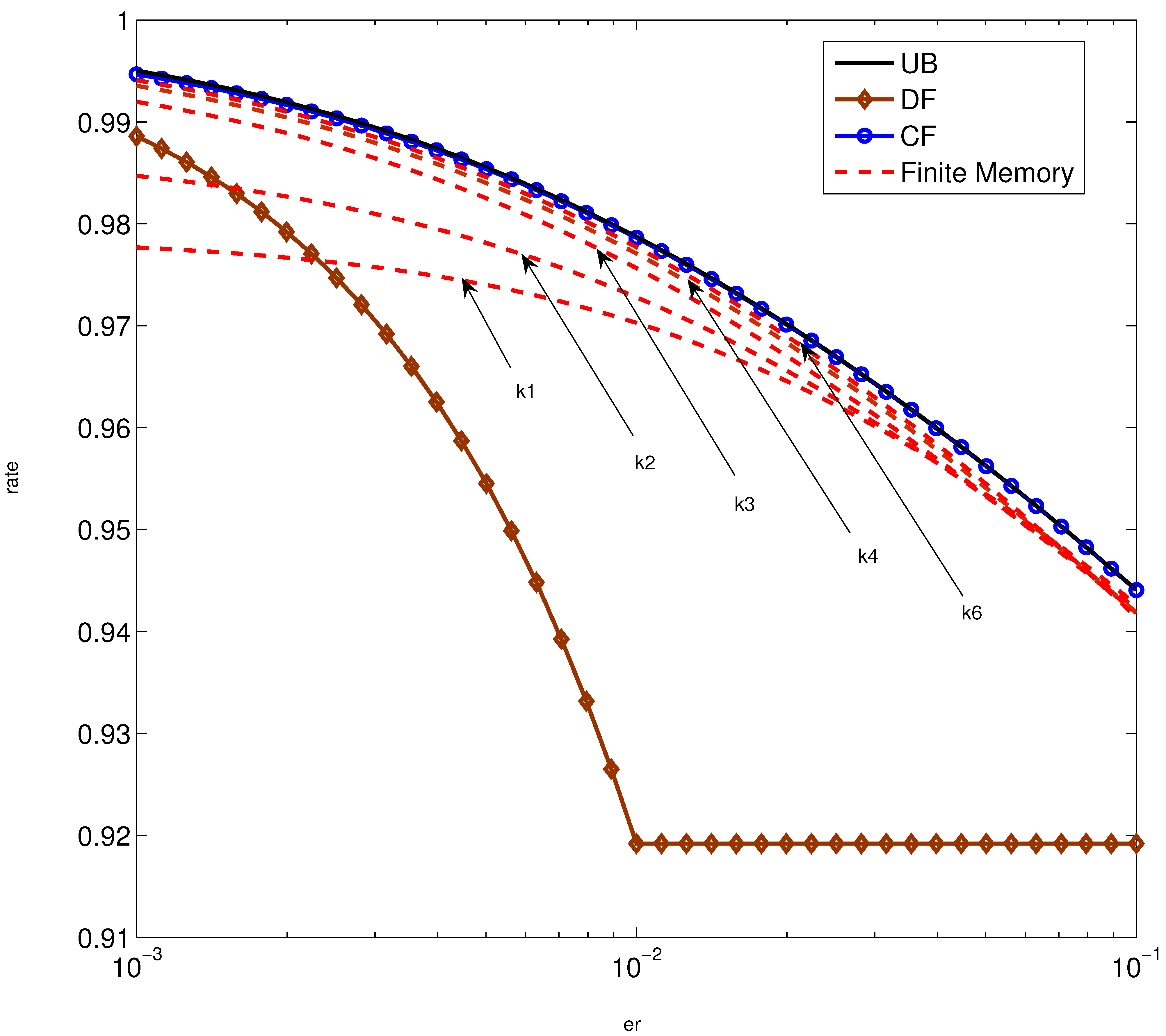
5. Numerical Examples

Figure 6 shows the capacity results for the orthogonal BSRC shown in Figure 2 as a function of ${ϵ}_r$ when ${ϵ}_1={ϵ}_2=0.01$. In this figure, we have plotted the cut-set upper bound (UB) (Equation (7)), rates achieved using decode-and-forward (DF) (Equation (8)), compress-and-forward (CF) (Equation (10)), and optimized finite memory relay (Equation (14)) for different memory size. The relay functions are optimized for the channel parameters ${ϵ}_1={ϵ}_2={ϵ}_r=0.01$ and are given in Table 1.

From Figure 6, we see that the achievable rate of DF decreases as ${ϵ}_r$ increases to $0.01$. For ${ϵ}_r\ge 0.01$, the achievable rate of DF coincides with that achievable with direct transmission (i.e., the relay is off). On the other hand, the rates achieved by CF coincides with the upper bound for the chosen channel parameters since the condition in Corollary 2 is satisfied. More interestingly, optimized low-dimensional relaying with $k=6$ achieves rates close to those achieved by CF and operates close to the capacity.

Figure 6. Capacity results for the binary symmetric relay channel as a function of ${ϵ}_r$ when ${ϵ}_1={ϵ}_2=0.01$.

Figure 6. Capacity results for the binary symmetric relay channel as a function of ${ϵ}_r$ when ${ϵ}_1={ϵ}_2=0.01$.

6. Summary and Concluding Remarks

We introduced a binary symmetric relay channel with orthogonal components at the destination, and investigated three main relaying strategies: decode-and-forward (DF) relaying, compress-and-forward (CF) relaying, and optimized low-dimensional relaying. We used a bit-switching numerical algorithm to find optimized mappings. We initialized our algorithm with arbitrary random nonlinear mappings, and after optimization based on Fourier analysis, we observed that all optimized mappings that we found were linear. We also illustrated that one can obtain rates very close to the upper bound by using the proposed optimized low-dimensional relaying scheme. It is worth noting that DF and CF require codebooks with infinite block length codewords at the relay. This stands in a sharp contrast to the proposed low-dimensional relaying scheme. Additionally, the suggested relaying protocol has low-delay processing and paves the way for implementation of inexpensive relaying protocols. We finally note that the sufficiency of linear mappings for the problem of optimal relaying remains open.

References

1. van der Meulen, E.C. Three-terminal communication channels. Adv. Appl. Probab. 1971, 3, 120–154. [Google Scholar] [CrossRef]
2. Cover, T.M.; El Gamal, A. Capacity theorems for the relay channel. IEEE Trans. Inform. Theory 1979, 25, 572–584. [Google Scholar] [CrossRef]
3. Høst-Madsen, A.; Zhang, J. Capacity bounds and power allocation for wireless relay channels. IEEE Trans. Inform. Theory 2006, 51, 2020–2040. [Google Scholar] [CrossRef]
4. El Gamal, A.; Mohseni, M.; Zahedi, S. Bounds on capacity and minimum energy-per-bit for AWGN relay channels. IEEE Trans. Inform. Theory 2006, 52, 1545–1561. [Google Scholar] [CrossRef]
5. Kramer, G.; Gastpar, M.; Gupta, P. Cooperative strategies and capacity theorems for relay networks. IEEE Trans. Inform. Theory 2005, 51, 3037–3063. [Google Scholar] [CrossRef]
6. Dabora, R.; Servetto, S.D. On the role of estimate-and-forward with time sharing in cooperative communication. IEEE Trans. Inform. Theory 2008, 541, 4409–4431. [Google Scholar] [CrossRef]
7. Laneman, J.N.; Wornell, G.W.; Tse, D.N.C. Cooperative diversity in wireless networks: Efficient protocols and outage behavior. IEEE Trans. Inform. Theory 2004, 50, 3062–3080. [Google Scholar] [CrossRef]
8. Sendonaris, A.; Erkip, E.; Aazhang, B. User cooperation diversity-Part I: System description. IEEE Trans. Commun. 2003, 51, 1927–1938. [Google Scholar] [CrossRef]
9. Sendonaris, A.; Erkip, E.; Aazhang, B. User cooperation diversity-Part II: Implementation aspects and performance analysis. IEEE Trans. Commun. 2003, 51, 1939–1948. [Google Scholar] [CrossRef]
10. Aleksic, M.; Razaghi, P.; Yu, W. Capacity of a class of modulo-sum relay channels. IEEE Trans. Inform. Theory 2009, 55, 921–930. [Google Scholar] [CrossRef]
11. Kim, Y.H. Coding Techniques for Primitive Relay Channels. In Proceedings of the Forty-Fifth Annual Allerton Conference, Allerton House, UIUC, IL, USA, 26–28 September 2007.
12. Lau, A.P.T.; Cui, S. Joint power minimization in wireless relay channels. IEEE Trans. Wirel. Commun. 2007, 6, 2820–2824. [Google Scholar]
13. Karystinos, G.N.; Liavas, A.P. Outage Capacity of a Cooperative Scheme with Binary Input and a Simple Relay. In Proceedings of the IEEE ICASSP 2008-International Conference Acoustics, Speech and Signal Processing, Las Vegas, NV, USA, 31 March– 4 April 2008.
14. Sagar, Y.; Kwon, H.M.; Ding, Y. Capacity of Modulo-Sum Simple Relay Network. In Proceedings International Zurich Seminar on Communications, Zurich, Switzerland, 3–5 March 2010.
15. El Gamal, A.; Aref, M. The capacity of the semi-deterministic relay channel. IEEE Trans. Inform. Theory 1982, 28, 536. [Google Scholar] [CrossRef]
16. Khormuji, M.N.; Larsson, E.G. Rate-optimized constellation rearrangement for the relay channel. IEEE Commun. Lett. 2008, 12, 618–620. [Google Scholar] [CrossRef]
17. Khormuji, M.N.; Skoglund, M. Piecewise linear relaying: Low complexity parametric relaying. In Proceedings of the IEEE SPAWC, Perugia, Italy, 21–24 June 2009.
18. Khormuji, M.N.; Skoglund, M. On instantaneous relaying. IEEE Trans. Inform. Theory 2010, 56, 3378–3394. [Google Scholar] [CrossRef]
19. Zaidi, A.; Khormuji, M.N.; Yao, S.; Skoglund, M. Rate-maximizing Mappings for Memoryless Relaying. In Proceedings of the IEEE ISIT, Seoul, Korea, 28 June–3 July, 2009.
20. Skoglund, M. On channel-constrained vector quantization and index assignment for discrete memoryless channels. IEEE Trans Inform. Theory 1999, 45, 2615–2622. [Google Scholar] [CrossRef]
21. Mehes, A.; Zeger, K. Performance of quantizers on noisy channels using structured families of codes. IEEE Trans. Inform. Theory 2000, 46, 2468–2476. [Google Scholar]
22. Rudin, W. Fourier Analysis on Groups; John Wiley And Sons Ltd: Hoboken, NJ, USA, 1990. [Google Scholar]
23. Khormuji, M.N.; Skoglund, M. On the Capacity of the Binary Symmetric Relay Channel with a Finite Memory Relay. In Proceedings of the IEEE ITW, Cairo, Egypt, 6–8 January 2010.
24. Liavas, A. Outage Capacity of a Cooperative Scheme with Binary Input and a Simple Relay. Year-1 Work-Package-1 report of European Commission FET Project FP6-033533-COOPCOM, November 2007. [Google Scholar]