Article

Maximum Entropy Gibbs Density Modeling for Pattern Classification

1
Laboratoire de recherche en imagerie et orthopédie, Centre de recherche du CHUM, École de technologie supérieure, Pavillon J.A. de Sève, 1560, rue Sherbrooke E., Y-1615, Montreal (QC),H2L 4M1, Canada
2
Institut national de la recherche scientifique, INRS-EMT, Place Bonaventure, 800, de La Gauchetière O., Montreal (QC), H5A 1K6, Canada
3
École de technologie supérieure, 1100, Rue Notre-Dame O., Montreal (QC), H3C 1K3, Canada
*
Author to whom correspondence should be addressed.
Entropy 2012, 14(12), 2478-2491; https://doi.org/10.3390/e14122478
Submission received: 25 September 2012 / Revised: 19 October 2012 / Accepted: 30 November 2012 / Published: 4 December 2012
(This article belongs to the Special Issue Maximum Entropy Production)

Abstract

:
Recent studies have shown that the Gibbs density function is a good model for visual patterns and that its parameters can be learned from pattern category training data by a gradient algorithm optimizing a constrained entropy criterion. These studies represented each pattern category by a single density. However, the patterns in a category can be so complex as to require a representation spread over several densities to more accurately account for the shape of their distribution in the feature space. The purpose of the present study is to investigate a representation of visual pattern category by several Gibbs densities using a Kohonen neural structure. In this Gibbs density based Kohonen network, which we call a Gibbsian Kohonen network, each node stores the parameters of a Gibbs density. Collectively, these Gibbs densities represent the pattern category. The parameters are learned by a gradient update rule so that the corresponding Gibbs densities maximize entropy subject to reproducing observed feature statistics of the training patterns. We verified the validity of the method and the efficiency of the ensuing Gibbs density pattern representation on a handwritten character recognition application.

Graphical Abstract

1. Introduction

It is common in scientific investigations to view measurement data as a sample drawn from a probability density function. The first step is then to use some of this data (called estimation data, or training data) and any other prior information to estimate this probability density function, to be used in the processing of subsequently acquired measurements. Usually, we do not know what the probability structure of the data is, and direct estimation faces a serious obstacle called the curse of dimensionality [1,2], because it is generally impractical to gather the necessary amount of estimation data when its dimensionality is large. In pattern classification, it is not unusual that the data is in the form of vectors of tens of entries, each entry representing a characteristic feature of the processed patterns. As a result, direct estimation is avoided and a parametric form of the density function is assumed. The problem is then to use the training data to estimate the parameters. Although a parametric representation lessens the problem significantly, it is quite important to assume a parametric form complex enough to be descriptive of the probability structure of the data. The uniform and the normal densities are often used for mathematical convenience. However, these models are often not applicable the data. The normal density, in its generality, has also the disadvantage of requiring a large number of parameters for patterns of high dimensionality ( n 2 / 2 + n ) for the covariance matrix and n for the mean, where n is the dimension of the random vector).
Several studies [3,4,5,6] have shown that the Gibbs density can model visual pattern data of complex probability structure, and described an efficient algorithm to estimate its parameters from training data. The Gibbs distribution results from a formulation that seeks the most neutral density function (i.e., of maximum entropy in the space of allowable densities) that reproduces all of the observed (i.e., chosen) statistics of the data; the statistics are histograms (empirical marginal distributions) of the features considered characteristic of the patterns for which the probability density model is sought. Under this formulation, the estimated density function does not differ from the true density as far as the chosen statistics are concerned, and does not embed other (unwanted) statistics. The Gibbs parameter estimation algorithm in [3,6] performs a gradient algorithm to maximize the constrained entropy criterion of the formulation. It has shown impressive results for texture and shape synthesis [3,5,6], where the goal was to generate texture or shape patterns resembling given examples. It has also been applied to character classification [7], a notoriously difficult problem. In pattern recognition, however, it is often the case that the structure of the pattern data to model is too complex to describe properly by a single parametric probability density function [1]. In such cases, it would be beneficial to represent the data using several parametric density functions to more accurately account for the shape of their distribution in the feature space [1].
The representation of patterns by histograms of features can be an issue in some applications. The measurements available that characterize the patterns under consideration may not allow a construction of histograms that the theory requires. For instance, the theory does not apply to descriptions by sets of scalar attributes, such as those provided in popular image classification databases (e.g., the IRIS and the Car Evaluation databases in the repository for machine learning research). Therefore, the description of patterns by histograms of feature measurements has its advantages and shortcomings: It affords a powerful description of patterns via Gibbs density modeling, as shown by the experimentations of Zhu et al. [5,6], but at the same time relies on a set of measurements on each individual shape large enough to allow the construction of a histogram.
The purpose of our study is to investigate visual pattern category representation by Gibbs densities using a Kohonen neural network. We will refer to this Gibbs density based Kohonen network as a Gibbsian Kohonen network. Trained on a sample of a given pattern, the Gibbsian Kohonen network that we propose will compute at each of its node the parameters of a Gibbs density. These Gibbs densities will serve, collectively, to model the pattern category. The parameters are computed by the network training algorithm in agreement with the gradient update rule that maximizes the constrained entropy criterion in [3,6]. The update rule at each node is a one training sample at a time version of this gradient update rule. Once the network is trained, each node contains the parameters of a Gibbs density that describes a subset of the data. The subsets form a partition, i.e., they are distinct and cover the training data. We verified the validity and efficiency of the network on a handwritten character classification application. We conducted experiments showing that the network affords an accurate representation of character category, more accurate than the Gibbs density learned by the procedure in [3,6,7].
The remainder of this paper is organized as follows: Section 2 reviews density estimation by constrained maximum entropy. This explains and puts in context the Gibbsian Kohonen network training algorithm, which is described in Section 3. An experimental validation is described in Section 4. Section 5 contains a conclusion.

2. Density Estimation by Constrained Maximum Entropy

This section gives a summary of the constrained maximum entropy formalism, and of the ensuing algorithm to estimate class-conditional Gibbs distribution parameters [3,6] from a set of visual patterns. This will put the Gibbsian Kohonen network (Section 3) into context.
The formalism applies to category patterns described by histograms of characteristic features. These histograms, which are empirical marginal distributions of the category patterns, are called pattern statistics in [6]. Such a description is typical of visual patterns. For instance, the statistics in [6] were histograms of the output of image filters such as directional derivatives, difference of Gaussians, and Gabor filters, applied at every point of the image positional array. The studies in [3,7] represented the contour of a visual shape by histograms of curvature and derivatives of curvature [3], and difference of tangents [7], measured at sampling points on the contour.
Let { Γ i o b s , i = 1 , . . . , M } be a set of M training patterns of a given category, called observed patterns.
Let Φ o b s = { ϕ o b s ( β ) , β = 1 , . . . , K } be a set of pattern features and H o b s = { H o b s ( β ) , β = 1 , . . . , K } the set of corresponding histograms, according to some discretization of the features. For large samples, and a fine discretization, the sample histogram averages, called the observed statistics,
μ o b s ( β ) = 1 M i = 1 M H ( β ) ( Γ i o b s ) β = 0 , 1 , . . . , K
are good estimates of the expectations E f [ H ( β ) ( Γ ) ] , where E f is the expectation with respect to the underlying true density f ( Γ ) of the patterns viewed as random variables. To approximate f ( Γ ) , a probability model p ( Γ ) is constrained to reproduce the observed statistics, i.e.,
E p [ H ( β ) ( Γ ) ] = μ o b s ( β ) β = 1 , 2 , . . . , K
The maximum entropy principle affords an efficient principled means of determining an approximation p of f.
In the discrete case, the entropy S of a discrete random variable X, which can take values { x 1 , . . . , x n } with corresponding probabilities p ( x 1 ) , . . . , p ( x n ) , is defined as: S [ X ] = 1 n p ( x i ) l o g ( p ( x i ) ) . In the continuous case, the entropy of a continuous random variable X with probability density function (pdf) p, is written as S [ X ] = p log p d X .
In our case, let Γ E , where E is the space of allowable shapes, and let Ω p be the set of distributions which reproduce the observed statistics,
Ω p = { p ( Γ ) | E p [ H ( β ) ( Γ ) ] = μ o b s ( β ) , β = 1 , 2 , . . . , K }
The maximum entropy principle prescribes that a good choice p * of the probability distribution is the one that has maximum entropy [6], i.e.,:
p * ( Γ ) = arg max p { - p ( Γ ) log p ( Γ ) d Γ }
subject to the following constraints:
p ( Γ ) d Γ = 1
E p [ H ( β ) ( Γ ) ] = H ( β ) ( Γ ) p ( Γ ) d Γ = μ o b s ( β ) β = 1 , 2 , . . . , K
Basically, the formulation seeks an estimate p * of the underlying density f, which reproduces the observed statistics and is as neutral as possible in the sense that it does not embody any other information. The solution of this constrained optimization problem is a Gibbs density of the form [5]:
p ( Γ ; Λ ) = 1 Z e - β = 1 K < λ ( β ) , H ( β ) ( Γ ) >
where < . , . > denotes inner product; Z is the partition function, i.e., the function that normalizes p to integrate to 1.
A maximum likelihood estimate of the density parameters
Λ = ( λ ( 1 ) , λ ( 2 ) , . . . , λ ( K ) )
called potential functions, can be computed by gradient descent:
d λ ( β ) d t = E p ( Γ ; Λ ) [ H ( β ) ( Γ ) ] - μ o b s ( β ) , β = 1 , 2 , . . . , K
This gradient descent evolution equation of the parameters comes from substituting the Gibbs density form (6) in the entropy function and then differentiating the resulting expression with respect to the parameters [5]. At each step t (algorithmic time), the expected values E p ( Γ ; Λ ) [ H ( β ) ( Γ ) ] can be estimated by synthesizing samples Γ s y n from p ( Γ ; Λ ) and using the averages μ s y n ( β ) . In such a case, Equation 7 becomes:
d λ ( β ) d t = μ s y n ( β ) - μ o b s ( β ) , β = 1 , 2 , . . . , K
The Gibbsian Kohonen network we propose, to be described in detail in the next section, will use this gradient descent equation to learn the parameters of a Gibbs density at each of its nodes.

3. Gibbs Pattern Density Modeling by a Kohonen Network

Here following we describe the Gibbsian Kohonen network training algorithm. This algorithm basically implements Equation 8 on a set of training patterns. To make the presentation of the Gibbsian Kohonen network clearer, we first describe the traditional Kohonen network, the structure of which it uses. The presentation of both networks will be followed by an explanation of their main similarities and differences.

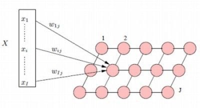
3.1. The Traditional Kohonen Network

The traditional Kohonen neural network [8], also called the Kohonen associative memory, and self-organizing map (SOM), has been the focus of an impressive number of studies in a variety of fields such as optimization, pattern recognition, image processing, and robotics. Several thousands of papers are listed in the bibliographies of [9,10].
The traditional Kohonen neural network implements a clustering algorithm similar to K-means [1,11,12]. It can be viewed as a vector quantizer, mapping large sets of data patterns onto a small computed set of patterns representative of pattern categories [13,14]. It can also be viewed as an associative memory, encoding input patterns in the form of weight vectors. It has the property of self organization because neighboring nodes can encode neighboring patterns.
The Kohonen algorithm has been modified to a probabilistic variant called probabilistic self-organizing map (PRSOM) [15]. The PRSOM associates to each network node a Gaussian density function to approximate the distribution of the input data using a mixture of normal distributions. However, with a large number of features, as it is often the case in pattern recognition [1], the Gaussian density has a large number of parameters and may not describe the patterns accurately enough [1].
Trained on a sample of a given pattern, the Gibbsian Kohonen network that we propose will compute at each of its node the parameters of a Gibbs density. These densities will serve, collectively, to model the pattern category. The parameters of this density are computed by the network training algorithm in agreement with the constrained entropy formalism [5] described in Section 2.

3.2. The Gibbsian Kohonen Network

The architecture of the Gibbsian Kohonen network is shown in Figure 1. Each node in this Gibbsian network stores the parameters of a Gibbs distribution learned from training samples in accordance with Equation 8. Assuming that the samples of a class of patterns contribute no information about other classes, a Kohonen memory is built for each class. The Gibbsian algorithm is described in Table 1. It runs as follows.
Figure 1. Kohonen neural networks.
Entropy 14 02478 g001
Table 1. The Gibbsian network training algorithm.
- Initialize the potential functions λ j ( β ) to small random values, β = 1 , . . . , K .
- Initialize patterns Γ j s y n in nodes j [ 1 , J ] .
- For n = 1 n i t e r , do
- For each training pattern Γ do
- Compute the vectors of representation H ( Γ ) and H ( Γ j s y n ) , j [ 1 , J ] .
- determine j * = min j d ( H ( Γ i ) , H ( Γ j s y n ) ) ,
- Update the potential functions:
λ j ( β ) ( n + 1 ) = λ j ( β ) ( n ) + ϵ n g n j , j * ( H ( β ) ( Γ j s y n ) - H ( β ) ( Γ i ) ) , β = 1 , . . . , K .
ϵ n = ϵ i ( ϵ f ϵ i ) n n m a x , g n j , j * = e x p - | | j - j * | | 2 2 σ n 2 , σ n = σ i ( σ f σ i ) n n m a x
- Synthesize new patterns Γ j s y n by MCMC using the potential functions
The potential functions
Λ j = ( λ j ( 1 ) , λ j ( 2 ) , . . . , λ j ( K ) )
stored at nodes j = 1 , . . . , J are first initialized to small random values. Let H i be the vector of feature histograms of the current input i, and let H j s y n the vector of feature histograms of the pattern synthesized by sampling a Gibbs distribution whose parameters are those stored currently at node j.
The synthesis is done by MCMC (Markov Chain Monte Carlo) stochastic sampling [3]. The sampling algorithm in the case of our online character classification application is given in the Appendix.
The node j * whose synthesized histogram vector is closest to the histogram vector of the current input is determined and the Gibbs parameters at each node j are updated in agreement with Equation 8, by an amount which is a decreasing function of the grid distance to node j * . Note that this update rule is a one sample at a time version of the gradient update in Equation 8. Function g j , j * defines the influence of node j * on node j during the update at j. At the iteration n:
g n j , j * = e x p - | | j - j * | | 2 2 σ n 2
σ n = σ i ( σ f σ i ) n n m a x
where n m a x is the maximum number of iterations.
g j , j * decreases with increasing grid distance between nodes j * and j and depends on parameter σ, which decreases with the number of iterations n between the values σ i and σ f . Parameter ϵ scales weight change and varies with the number of iterations from ϵ i to ϵ f . Parameters σ i , σ f , ϵ i and ϵ f must be chosen appropriately to obtain convergence of the iterations and topological ordering of the network. The values of the parameters used in our experiments are σ i = 1 , σ f = 0.02 , ϵ i = 1 , and ϵ f = 0.0005 .
Once the network for each class C l , l = 1 , . . . , L is trained, the classification can be done as follows: Let Γ be the pattern to classify and H its vector of feature histograms. Let d l be the minimum distance between H and the synthesized histograms in the trained Kohonen network for class C l . Pattern Γ is assigned to class k where
d k = min l d l

3.3. The Main Differences and Similarities

The Kohonen network and the Gibbsian Kohonen network have the same physical structure: an array (two-dimensional in this study) of code storing nodes, each connected to its neighbors according to a neighborhood system (the 4-neighborhood system in this study). The logical structure is also the same: each node performs an identical operation that consists of an update of its store modulated by its distance from the node closest to the current input. The main difference is the update rule. The Kohonen network update consists of pulling the stored value at each node toward the current input by an amount proportional to their difference. Ritter and Schulten have shown that this performs a Markov process with a potential function exhibiting numerous local minima [12]. In general, one cannot draw a conclusion on the distribution of the input falling in a node. Differently, the Gibbsian Kohonen network update rule determines the parameters of a Gibbs distribution to describe the input falling in a node. This update rule is a one sample at a time form of the gradient update in Equation 8. The use of one sample at a time variants of multi-sample update rules are common in pattern classification [1]. We recall from Section 2 that the multi-sample equation in this study (Equation 8) follows the maximization of a constrained entropy criterion (Equations 35) to determine a Gibbs distribution model of the input.
Another difference between the Kohonen network and the Gibbsian Kohonen network is the form of the input they process. The Gibbsian network runs an algorithm which applies to inputs in the form of histograms. These histograms are viewed as empirical realizations of the input data marginal distributions which the Gibbs distribution model is constrained to reproduce, while being the most neutral possible in the sense that it does not embody other information. A description by histograms of features is natural and common for images. In the study on texture modeling [5], for instance, the features resulted from the point-wise application of various filters such as spatial derivatives and Gabor filters. In the online character example of this study (next section), the pattern features are curvature approximation measurements at points along the acquired character signals.
The traditional Kohonen network and the Gibbsian Kohonen network have the same parameters to govern their logical structure, namely the coefficient ϵ i , ϵ f , σ i , and σ f used in the update equations of the algorithm described in Table 1. For both networks, these parameters are determined experimentally and in the same manner. Their value does not require fine tuning. For instance, in the on-line character recognition example of this study, the values in the range of those we determined in a previous study [13], and used in others [14,16,17], were fitting. There are other parameters associated indirectly to the Gibbsian Kohonen network via pattern synthesis which it used (last line in Table 1). These pertain to the MCMC shape sampling algorithm (Table 3), which is instantiated at each iteration of the algorithm of Table 2 and for each training pattern. Although the few parameters that this sampling algorithm uses can be quickly determined because they are discretization parameters, the shape sampling requires several iterations at each activation. Therefore, the last step of the Gibbsian network training algorithm is time consuming. However, it is important to bear in mind that the training algorithm is run only once, at the onset of the given application. Therefore, the training time requirement is not a decisive issue. Once the network is trained, it becomes a straightforward classifier with a classification time extremely short because it only involves computing a small set of vector distances and choosing the shortest.
Feature selection determines the number and type of features that are characteristic of the patterns in a category. It is part of any classification task regardless of the type of classifier used. It often involves parameter setting. Such parameters are not part of the intrinsic logical functions of the classifier in the sense that the classifier does not contain any operation destined to the choice of features. However, parameter setting is generally done by running the classifier with different values of the parameter and choosing the one that gives the best results. This can be time consuming but it is part of training, not classification proper, and, therefore, done only once. The Gibbsian network uses histograms of characteristics to describe the patterns of a category as will be discussed in more details in Section 4. The use of histograms has a two-sided implication. It is a powerful representation of patterns because they are empirical marginal distributions but, at the same time, the Gibbsian network depends on this representation exclusively, which restricts the type of features to use as input.

4. An Experimental Validation

We verified the Gibbsian Kohonen network algorithm and its implementation on handwritten online Arabic character recognition. In general, handwritten character data exhibits important inter- and intra-scriptor distortions, which make automatic classification a challenging task and, therefore, a good test to assess the potency of a classifier [18].

4.1. The Database

The data was collected using a Wacom Graphire digital tablet with a resolution accuracy of 23 points/cm and a sampling frequency of 100 points/s. The database contains 9504 handwritten characters collected from 22 writers, which represents 528 specimens of each of 18 isolated letters. Writing of the characters was not constrained, leading to a wide variety of sizes and orientations. Also, the database contains both clearly written characters and roughly written ones. This database was used and described in detail in [7]. For the experimental verification, the database was divided into two distinct sets. The training set contained 6336 samples and the testing set the remaining samples.

4.2. Feature Extraction

In accordance with the formalism of Section 2, we represented an online character by histograms of features, namely tangent differences computed from the character sequence of point coordinates as follows. Let ( ( x 0 , y 0 ) , ( x 1 , y 1 ) , · · · , ( x N - 1 , y N - 1 ) ) be the sequence of coordinates, and let θ k , k = 0 , . . . , N - 1 , be the tangent angles θ k = arctan ( y k + 1 - y k x k + 1 - x k ) , where indices are modulo N ( N = 50 in this application). For 1 α N - 1 , let ϕ ( α ) be the feature corresponding to the tangent angle differences defined by: ϕ ( α ) = θ k + α - θ k . Therefore, we have a set of features Φ = { ϕ ( α ) } , α = 1 , 2 , . . . , N . To each feature α corresponds a histogram H ( α ) following a discretization of the feature. Each seen as a vector, the histograms for all the features can be concatenated to form the vector of representation H, H ( Γ ) = ( H ( 1 ) ( Γ ) , H ( 2 ) ( Γ ) , . . . H ( N - 1 ) ( Γ ) ) . The use of all statistics H ( α ) , α { 0 , 1 , . . . , N - 1 } can result in a histogram representation H of significantly high dimension. For N = 50 and m = 36 , for instance, the representation has 1800 entries. Moreover, such a representation contains a significant amount of redundant information because features corresponding to close values of α have close histograms which, therefore, contain similar information about the shape Γ. Because neighboring features are highly correlated and the use of all the features results in a high dimensional vector, it is adequate to use a subset of K features. Trying all subsets of features to determine which one is best is, of course, of combinatorial complexity and, therefore, prohibitively expensive. However, it is sufficient, for our purpose, to have a reasonable set of features so as to concentrate on the problem of classification proper. We ran a substantial number of experiments with α equal to multiples of 2, 3, 4, and 5, and with the number of features K equal to 4, 5, 6, and 7. The number of histogram bins was varied between 8 and 36 by increments of 4 (to have reasonably distinct histogram representations). The best results, in terms of recognition rates, were obtained with K = 6 , multiples of 5 for α, and 12-bin histograms. We represented each character category by a 5 × 5 memory. Note that the histogram representation is determined for the whole database, rather than on a character category basis.

4.3. Evaluation

We evaluated performance by average recognition rates in L - fold cross validation experiments. We used L = 3 . Therefore, the database is divided into three disjoint parts of (approximately) equal size. Two parts serve training and the other part is used for testing. By varying the role of each part, we make three separate experiments, and recognition rates are averaged over these three experiments. If we assume that the number of samples in the database is a multiple of L, then, as pointed out in [18], L = 3 gives the least number of training samples strictly greater than the number of test samples. This value reflects the concern of training a classifier on as much data as possible and tests it on as much distinct data as possible under the constraint that the training sample is strictly larger than the test sample. In this case, recognition rates can be viewed as worst case rates compared with those with L > 3 .
The partition of the data into training and testing subsets was done as follow: (1) the test subset did not contain data from writers who contributed to the training subset, i.e., the validation is writer independent; and (2) the choice of which writer to include in which subset is done randomly. Therefore, this division of the data into training/testing offers an unbiased writer independent experimentation, which is not prone to statistical peculiarities that can be present in individual data sets.
Table 2 gives the Gibbsian network recognition rates for 3-fold validation. The average classification rate is 94.6 % . The relevant background to contrast these results to includes Bayes classification by class-conditional Gibbs density modeling [7] and the classical Kohonen network classification. In the comparison to follow, the parameters of each algorithm were optimized empirically. This, of course, can be a length procedure but pertains to training and, therefore done only once, at the onset of the application. The Kohonen training algorithm, using the histogram representation of characters is about 65 min on a relatively slow machine (SPARC ultra5, 360 MHz). The Gibbsian Kohonen network with the same representation required about five hours, which is 5 times the execution time of the traditional Kohonen network. Once trained the classification time of both network is of the order of the millisecond per character.
Table 2. 3-fold cross validation recognition rates using a 5 × 5 Gibbsian and Kohonen networks for each character category.
FoldGibbsian networkKohonen networkDifference
195.1 %94.4 %+0.7
294.0 %92.1 %+1.9
394.7 %92.4 %+2.3
Mean94.6%92.9 %+1.7
Bayes classification requires the class-conditional partition functions. The study [7] investigated two methods, one that uses the training data set directly and the other that draws samples from a reference distribution [19]. The performance of the corresponding Bayes decision methods were low ( 84.0 % and 89.87 % ) but a combination of the methods, which exploited their different error profiles, gave the good performance of 92.6 % recognition. The low performance of each of the Bayes methods is due in part to the difficulty to estimate the partition function, but mainly to the use of a single Gibbs density to model the category data.
The performance of the Gibbsian network compared with that of Gibbs Bayes classifiers is instructive because it shows the advantage of using several densities, rather than a single one, to represent pattern categories. However, it is also instructive to look at the performance of the traditional Kohonen network because it will show the pertinence of a Gibbs representation of patterns. To this effect, using the same character features and the same database, we ran experiments with a 5 × 5 (traditional) Kohonen memory for each character category. The 3-fold cross validation results are shown in Table 2. The average rate is 1.7 % lower than for the Gibbsian network, which is an important difference at this level of recognition (92%–94%) [1].
We have used the Ritter and Kohonen version of the original Kohonen network training algorithm. This continuous formulation is explained in the papers [12,20], which also give some theoretical results and examples. Our implementation has benefited from the prior investigations of [13,14,17,21] regarding the setting of the basic parameters intervening in training. In particular, Le Bail [13] has conducted extensive experimentation on these parameters. Typically, training can be tedious but otherwise uncomplicated.

4.4. Test of Statistical Significance

A statistical test of hypothesis to compare the Gibbsian and the Kohonen networks performance would be inconsequential if the recognition rates are used as the random events because such events are not independent. Indeed, the recognition rates are obtained in pairs by first sampling of the data and training and testing the classifiers on the samples. Instead, a more appropriate event to consider is the difference of the two classifiers performance for each random sampling of the data. In such a case, a random sampling of the data would correspond to a single hypothesis testing event, as it should. To this effect, both the Paired Student t-test and the Sign test are quite fitting. The Paired Student t-test yields that the difference in performance between the two classifiers (the Gibbsian network improving on the Kohonen network) is significant with a 90 % confidence interval for the mean recognition difference. The sign test leads the same conclusion. These statistical results fit well with intuition because the Gibbsian network performance is systematically higher in all the experiments (Table 2).

5. Conclusions

This study investigated a Kohonen neural network that can learn the parameters of Gibbs distributions to represent a pattern described by histograms (empirical distributions) of features considered descriptive of the category patterns. For each category, the Gibbsian Kohonen network computes at each of its node the parameters of a Gibbs density. The Gibbs densities at all nodes serve collectively to model the pattern category. The parameters are learned by a gradient update rule so as to maximize a constrained entropy criterion, leading to optimal densities that reproduce the observed characteristics of the training data. Once trained, the network functions as an associative memory to classify patterns, much like the traditional Kohonen network. This Gibbsian Kohonen network was tested on a character recognition application that shows better classification results than with the traditional Kohonen network. This work can benefit from an in-depth investigation of effective ways to estimate the partition functions of the Gibbs densities in the network.

Appendix

A. MCMC Shape Sampling Algorithm

The sampling process [3,22] starts with a given character shape
Γ = ( ( x 1 , y 1 ) , ( x 2 , y 2 ) , . . . ( x n p o i n t , y n p o i n t ) )
. At each step n, it considers a point A l ( x l , y l ) on the shape Γ and proposes to move it to a candidate point A l ( x l , y l ) in a local neighborhood of A l (Table A1). The proposal A l is accepted with probability
η ( Γ Γ s y n ) = min ( p ( Γ s y n ; Λ ) p ( Γ ; Λ ) , 1 )
If the ratio r = p ( Γ s y n ; Λ ) p ( Γ ; Λ ) is higher than 1, then the point candidate A l ( x l , y l ) is accepted. Otherwise, the point is accepted with a probability r. This algorithm synthesizes the shapes Γ s y n used to calculate potential functions Λ.
In order to improve the sampling process, we chose the candidate point A l among points A l d ( x l d , y l d ) by moving the point A l according to the directions d,
x l d = x l + τ sin ( κ d ) , y l d = y l + τ cos ( κ d )
where κ d indicates the angle corresponding to direction d. κ d = d 2 π n d i r e c t i o n and τ is a scale factor calculated according to τ = d s c o n s t a n t , d s being the length of the segment between two consecutive points of the form Γ. We chose a code with eight directions ( n d i r e c t i o n = 8 ), and a c o n s t a n t equal to 5 for the calculation of the scale factor τ.
Table A1. Shape sampling algorithm.
Given a shape Γ = ( ( x 1 , y 1 ) , ( x 2 , y 2 ) , . . . ( x n p o i n t , y n p o i n t ) )
- For s = 1 s m a x , with s m a x being the maximum sweep number
- For p = 1 n p o i n t ,with n p o i n t being the point number on shapes
- For d = 1 n d i r e c t i o n ,
with n d i r e c t i o n being the number of
directions
- move A l according to d directions
to obtain a set of new shapes Γ d ,
l = 1 , 2 , . . . , d
- Compute p ( Γ d ; Λ ) by Equation (6).
- Keep Γ ^ which maximizes p ( Γ d ; Λ ) and affect it to Γ s y n .
- Compute η ( Γ Γ s y n ) = min ( p ( Γ s y n ; Λ ) p ( Γ ; Λ ) , 1 ) .
- Draw a random number r [ 0 , 1 ] from a uniform distribution
- If r < η , replace Γ by Γ s y n .

References

  1. Duda, P.O.; Hart, P.E.; Stork, D.G. Pattern Classification. New York, NY, USA, 2001. [Google Scholar]
  2. Jain, A.; Duin, R.; Mao, J. Statistical pattern recognition: A review. IEEE Trans. Pattern Recognit. Mach. Intell. 2000, 22, 4–37. [Google Scholar] [CrossRef]
  3. Zhu, S. Embedding gestalt laws in Markov random fields. IEEE Trans. Pattern Recognit. Mach. Intell. 1999, 21, 1170–1187. [Google Scholar]
  4. Zhu, S.C.; Mumford, D. Prior learning and Gibbs reaction-diffusion. IEEE Trans. Pattern Recognit. Mach. Intell. 1997, 19, 1236–1250. [Google Scholar]
  5. Zhu, S.C.; Wu, Y.; Mumford, D. Minimax entropy principle and its application to texture modeling. Neural Comput. 1997, 9, 1627–1660. [Google Scholar] [CrossRef]
  6. Zhu, S.C.; Wu, Y.; Mumford, D. Filters, Random Fields and Maximum Entropy (FRAME): Towards a unified theory for texture modeling. Int. J. Comput. Vision 1998, 27, 107–126. [Google Scholar] [CrossRef]
  7. Mezghani, N.; Mitiche, A.; Cheriet, M. Bayes classification of online arabic characters by Gibbs modeling of class conditional densities. IEEE Trans. Pattern Recognit. Mach. Intell. 2008, 30. [Google Scholar] [CrossRef] [PubMed]
  8. Kohonen, T. Self-organizing Maps; Springer: Berlin/Heidelberg, Germany, 1995. [Google Scholar]
  9. Kaski, S.; Kangas, J.; Kohonen, T. Bibliography of Self-Organizing Map SOM papers: 1981–1997. Neural Comput. Surveys 1998, 1, 102–350. [Google Scholar]
  10. Oja, M.; Kaski, S.; Kohonen, T. Bibliography of Self-Organizing Map SOM papers: 1998–2001 addendum. Neural Comput. Surveys 2003, 3, 1–156. [Google Scholar]
  11. Lippman, R. An introduction to computing with neural networks. IEEE ASSP Mag. 1987, 3, 4–22. [Google Scholar] [CrossRef]
  12. Ritter, H.; Schulten, K. 1988. Kohonen Self-Organizing Maps: Exploring Their Computational Capabilities. In Proceedings of the IEEE International Joint Conference on Neural Networks, Piscataway, NJ, USA, 1988; IEEE Service Center. Volume I, pp. 109–116.
  13. LeBail, E.; Mitiche, A. Quantification vectorielle d’images par le réseau neuronal de kohonen. Traitement du Signal 1989, 6, 529–539. [Google Scholar]
  14. Sabourin, M.; Mitiche, A. Modeling and classification of shape using a Kohonen associative memory with selective multiresolution. Neural Netw. 1993, 6, 275–283. [Google Scholar] [CrossRef]
  15. Anouar, F.; Badran, F.; Thiria, S. Probabilistic self-organizing map and radial basis function. J. Neurocomput. 1998, 20, 83–96. [Google Scholar] [CrossRef]
  16. Mezghani, N.; Mitiche, A.; Cheriet, M. On-line Recognition of Handwritten Arabic Characters Using a Kohonen Neural Network. In Proceedings of the 8th International Workshop on Frontiers in Handwriting Recognition, Niagara-on-the-Lake, Canada, 6–8 August 2002; pp. 490–495.
  17. Mezghani, N.; Mitiche, A.; Cheriet, M. A new representation of shape and its use for superior performance in on-line Arabic character recognition by an associative memory. Int. J. Doc. Anal. Recognit. 2005, 7, 201–210. [Google Scholar] [CrossRef]
  18. Mitiche, A.; Aggarwal, J. Pattern category assignement by neural networks and the nearest neighbors rule. Int. J. Pattern Recognit. Artif. Intell. 1996, 10, 393–408. [Google Scholar] [CrossRef]
  19. Descombes, X.; Morris, R.; Zerubia, J.; Berthod, M. Maximum Likelihood Estimation of Markov Random Field Parameters Using Markov Chain Monte Carlo Algorithms. In Proceedings of the Internalional Workshop on Energy Minimization Methods, Venice, Italy, 21–23 May 1998.
  20. Ritter, H.; Kohonen, T. Self-organizing semantic maps. Biol. Cybern. 1989, 61, 241–254. [Google Scholar] [CrossRef]
  21. Mezghani, N.; Phan, P.; Mitiche, A.; Labelle, H.; de Guise, J. A Kohonen neural network description of scoliosis fused region and their corresponding lenke classification. Int. J. Comput. Assist. Radiol. Surgery 2012, 7, 157–264. [Google Scholar] [CrossRef] [PubMed]
  22. Spall, J.C. Estimation via Markov Chain Monte Carlo. IEEE Control Syst. Mag. 2003, 23, 34–45. [Google Scholar] [CrossRef]

