1. Introduction
The principles and methods in Shannon’s information theory have been widely applied in statistical estimation, filtering, and learning problems [
1,
2,
3,
4,
5,
6,
7,
8,
9,
10,
11,
12,
13,
14,
15,
16,
17,
18]. The learning process is essentially a procedure of information processing with the goal of decreasing data redundancy in the presence of uncertainty and encoding the data into a model, and hence it is intrinsically related to information theory. An information theoretic description of learning processes was given in [
10], where learning is defined as a process in which the system’s subjective entropy or, equivalently, its missing information decreases in time. The mathematical concept of information was also brought to biologically plausible information processing [
11]. In addition, a unifying framework for information theoretic learning (ITL) has been presented in [
18].
From a statistical viewpoint, learning can be thought of as approximating the
a posteriori distribution of the targets given a set of examples (training data).
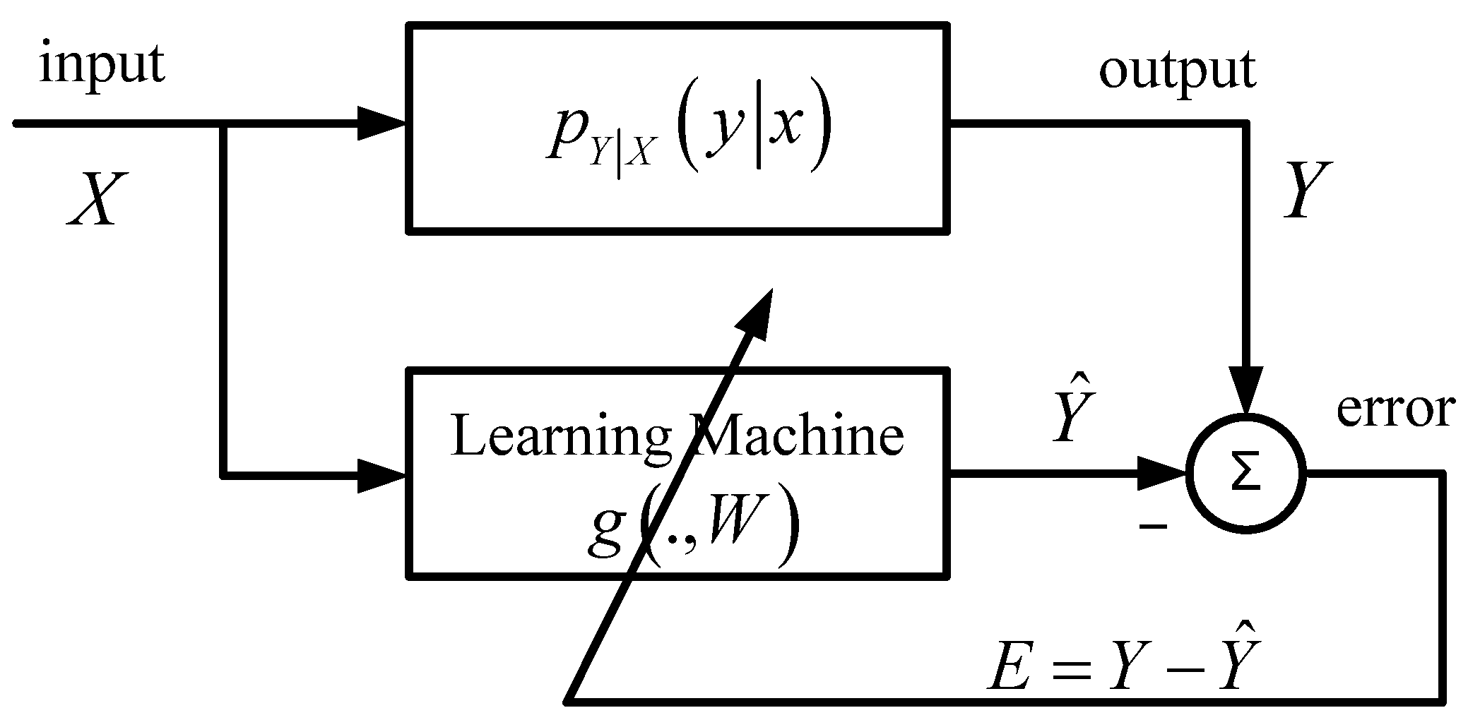
Figure 1 shows a general scheme of supervised machine learning, where the desired system output
Y (the teacher) is assumed to be related to the input signal
X through a conditional probability density function (PDF)
, and the learning machine (model) is represented by a parametric mapping
g (.,
W), where
denotes a parameter vector that needs to be estimated.
Figure 1.
A general scheme of supervised machine learning.
Figure 1.
A general scheme of supervised machine learning.
The learning goal is then to adapt the parameter
W such that the discrepancy between the model output
and the desired output
Y is minimized. How to measure the discrepancy (or model mismatch) is a key aspect in learning. One can use a statistical descriptor of the error (
) distribution as the measure of discrepancy. The most popular descriptors are the second order moments (variance, correlation,
etc.), which combined with the Gaussian assumption, in general leads to mathematically convenient and analytically tractable optimal solutions. A typical example is the mean square error (MSE) criterion in least-squares regression. However, the second order statistics as optimality criteria may perform poorly especially in nonlinear and non-Gaussian (e.g., heavy-tail or finite range distributions) situations. Recently, the error entropy, as an information theoretic alternative to MSE, has been successfully applied in supervised adaptive system training [
12,
13,
14,
15,
16,
17]. The minimum error entropy (MEE) criterion usually outperforms MSE criterion in many realistic scenarios, since it captures higher-order statistics and information content of signals rather than simply their energy. Under the MEE criterion, the optimal weight in
Figure 1 will be:
where
H (
E) denotes the Shannon entropy of the error
E,
pE(.) denotes the error PDF, and
denotes the expectation operator. Throughout this paper, “log” denotes the natural logarithm. The formulation (1) can be generalized to other entropy definitions, such as the
α-order Renyi entropy [
18]. Since entropy is shift invariant, the error PDF
pE(.) is in general restricted to zero mean in practice.
The learning machine in
Figure 1 can also be a nonparametric and universal mapping
g(.). Familiar examples include the support vector machine (SVM) [
19,
20] and kernel adaptive filtering [
21]. In this case, the hypothesis space for learning is in general a high (possibly infinite) dimensional reproducing kernel Hilbert space (RKHS)
, and the optimal mapping under MEE criterion is:
To implement the MEE learning, we should evaluate the error entropy. In practice, however, the error distribution is usually unknown, and the analytical evaluation of error entropy is not possible. Thus we have to estimate the error entropy from the samples. One simple way is to estimate the error PDF based on available samples, and plug the estimated PDF directly into the entropy definition to obtain the entropy estimator. In the literature there are many techniques for estimating the PDF of a random variable based on its sample data. In ITL, the most widely used approach is the Parzen windowing (or kernel density estimation) [
22]. By Parzen windowing, the estimated error PDF is:
where
is the kernel function with smoothing factor (or kernel size)
λ > 0,
is a continuous density, and
are error samples which are assumed to be independent and identically distributed (i.i.d.). As sample number
N → ∞, the estimated PDF will uniformly converge (with probability 1) to the true PDF convolved with the kernel function, that is
where * denotes the convolution operator. Then, by the Parzen windowing approach (with a fixed kernel function
), the estimated error entropy will converge almost surely (a.s.) to the entropy of the convolved density (see [
22,
23]). Thus, the actual entropy to be minimized is:
where
Z denotes a random variable that is independent of
X,
Y,
E, and has PDF
. Note that the PDF of the sum of two independent random variables equals the convolution of their individual PDFs. Here, we call the entropy
H (
E +
λZ) the smoothed error entropy, and
Z the smoothing variable. Under the smoothed MEE (SMEE) criterion, the optimal mapping in (2) becomes:
Although SMEE is an actual learning criterion (as sample number
N → ∞) in ITL, up to now its theoretical properties have been little studied. In this work, we study theoretically the SMEE criterion. The rest of the paper is organized as follows: in
Section 2, we present some basic properties of the SMEE criterion. In
Section 3, we investigate how the smoothing factor
λ affects the optimal solution. Finally in
Section 4, we give the conclusion.
2. Some Basic Properties of SMEE Criterion
In this section, some basic properties of SMEE criterion are presented. We assume from now on, without explicit mention, that the learning machine is a nonparametric and universal mapping g(.). In addition, the input vector X belongs to an m-dimensional Euclidean space, , and for simplicity, the output Y is assumed to be a scalar signal, .
Property 1: Minimizing the smoothed error entropy will minimize an upper bound of the true error entropy H (E).
Proof: According to the entropy power inequality (EPI) [
1], we have:
Thus, minimizing the smoothed error entropy H (E + λZ) minimizes an upper bound of H (E).
Remark 1: Although this property does not give a precise result concerning SMEE vs. MEE, it suggests that minimizing the smoothed error entropy will constrain the true error entropy to small values.
Property 2: The smoothed error entropy is upper bounded by , where and denote the variances of E and Z, respectively, and this upper bound is achieved if and only if both E and Z are Gaussian distributed.
Proof: The first part of this property is a direct consequence of the maximum entropy property of the Gaussian distribution. The second part comes from Cramer’s decomposition theorem [
24], which states that if
X1 and
X2 are independent and their sum
X1 +
X2 is Gaussian, then both
X1 and
X2 must also be Gaussian.
Remark 2: According to Property 2, if both E and Z are Gaussian distributed, then minimizing the smoothed error entropy will minimize the error variance.
Property 3: The smoothed error entropy has the following Taylor approximation around
λ = 0:
where
o (
λ2) denotes the higher-order infinitesimal term of Taylor expansion, and
J (
E) is the Fisher information of
E, defined as:
Proof: This property can be easily proved by using De Bruijn’s identity [
25]. For any two independent random variables
X1 and
X2,
, De Bruijn’s identity can be expressed as
where
denotes the variance of
X2 (Classical deBruijn identity assumes that
X2 is Gaussian. Here, we use a generalized deBruijn identity for arbitrary (not necessarily Gaussian)
X2 [
25]). So, we have:
and hence, we obtain the first-order Taylor expansion:
Remark 3: By Property 3, with small
λ, the smoothed error entropy equals approximately the true error entropy plus a scaled version of the Fisher information of error. This result is very interesting since minimizing the smoothed error entropy will minimize a weighted sum of the true error entropy and the Fisher information of error. Intuitively, minimizing the error entropy tends to result in a spikier error distribution, while minimizing the Fisher information makes the error distribution smoother (smaller Fisher information implies a smaller variance of the PDF gradient). Therefore, the SMEE criterion provides a nice balance between the spikiness and smoothness of the error distribution. In [
26], the Fisher information of error has been used as a criterion in supervised adaptive filtering.
Property 4: Minimizing the smoothed error entropy H (E + λZ) is equivalent to minimizing the mutual information between E + λZ and the input X, i.e., .
Proof: Since mutual information
, where
denotes the conditional entropy of
X given
Y, we derive:
where (a) comes from the fact that the conditional entropy
does not depend on the mapping
g(.).
Property 5: The smoothed error entropy is lower bounded by the conditional entropy , and this lower bound is achieved if and only if the mutual information I (E + λZ; X) = 0.
Proof: As
, we have:
where (b) is because of the non-negativeness of the mutual information
I (
E +
λZ;
X).
Remark 4: The lower bound in Property 5 depends only on the conditional PDF of
Y given
X and the kernel function
, and is not related to the learning machine. Combining Property 5 and Property 2, the smoothed error entropy satisfies the following inequalities:
Property 6: Let
be the smoothed conditional PDF of
Y given
X =
x, where the convolution is with respect to
y. If for every
,
is symmetric (not necessarily about zero) and unimodal in
, then the optimal mapping in (6) equals (almost everywhere):
where
is any constant.
Proof: The smoothed error PDF
can be expressed as:
where
F(
x) denotes the distribution function of
X. From (18), we see that the SMEE criterion can be formulated as a problem of shifting the components of a mixture of the smoothed conditional PDFs so as to minimize the entropy of the mixture. Then Property 6 holds since it has already been proved in [
27] that, if all components (conditional PDFs) in the mixture are symmetric and unimodal, the conditional mean (or median) will minimize the mixture entropy. The constant
c is added since the entropy is shift-invariant (in practice we usually set
c = 0).
3. How Smoothing Factor Affects the Optimal Solution
The smoothing factor λ is an important parameter in SMEE criterion, which controls the smoothness of the performance surface. In the following, we will investigate how the smoothing factor affects the optimal solution (optimal mapping) g*(.).
When λ = 0, the smoothed error entropy becomes the true error entropy, and the SMEE criterion reduces to the original MEE criterion. When λ > 0, the two criteria are different and, in general have different solutions. However, in some situations, for any λ, the SMEE criterion yields the same solution as the MEE criterion.
Proposition 1: If the desired output
Y is related to the input signal
X through the nonlinear regression model
Y =
f(
X) +
N, where
f is an unknown nonlinear mapping, and
N is an additive noise that is independent of
X and
Z, then for any
λ, the optimal solution under SMEE criterion is:
Proof: For any mapping
, and any
λ, we have:
where
U =
f(
X) −
g(
X),
V =
N +
λZ, and (c) comes from the fact that
U and
V are independent. The equality in (20) holds if and only if
U is
δ distributed, that is,
U is a constant. This can be easily proved as follows.
If
U is a constant, the equality in (20) will hold. Conversely, if the equality in (20) holds, we can prove that
U is a constant. Actually, in this case,
U and
U +
V are independent, and hence,
. It follows that:
which implies that the variance of
U is zero (
i.e.,
U is a constant). Therefore we have
g*(
x) =
f(
x) +
c.
Remark 5: Proposition 1 implies that for the nonlinear regression problem, the optimal solution under the SMEE criterion does not change with the smoothing factor provided that the additive noise is independent of the input signal.
If the unknown system (the conditional PDF) is not restricted to a nonlinear regression model, under certain conditions the optimal solution of SMEE can still remain unchanged with the smoothing factor λ. Specifically, the following proposition holds.
Proposition 2: If the conditional PDF
and the kernel function
are both symmetric (not necessarily about zero) and both unimodal in
, then for any
λ, the SMEE criterion produces the same solution:
Proof: By Property 6, it suffices to prove that the smoothed conditional PDF
is symmetric and unimodal. This is a well-known result and a simple proof can be found in [
28].
Remark 6: Note that the optimal solution under the minimum error variance criterion is also given by (22). In particular, if setting c = 0, the solution (22) becomes the conditional mean, which corresponds to the optimal solution under the MSE criterion.
Proposition 3: Assume that the conditional PDF is symmetric (not necessarily unimodal) with uniformly bounded support, and the kernel function is a zero-mean Gaussian PDF with variance λ2. Then, if smoothing factor λ is larger than a certain value, the optimal solution under the SMEE is still given by (22).
Proof: By Property 6, it is sufficient to prove that if smoothing factor
λ is larger than a certain value, the smoothed conditional PDF
is symmetric and unimodal. Suppose without loss of generality that the conditional PDF
is symmetric about zero with bounded support [-
B,
B],
B > 0. Since kernel function
is a zero-mean Gaussian PDF with variance
λ2, the smoothed PDF
can be expressed as:
where (d) follows from
. Clearly,
is symmetric in
y. Further, we derive:
We give below a simple proof of (25). It suffices to consider only the case
y ≥ 0 In this case, we consider two subcases:
- (1)
y ≥
B: In this case, we have
, (
y - τ) ≥ 0, and hence:
- (1)
(2) 0 ≤
y <
B: In this case, we have
,
. Since
:
we have
, and it follows easily that:
Combining (24), (26) and (28), we get , . Therefore (25) holds, which implies that if λ ≥ 2B the smoothed PDF is symmetric and unimodal, and this completes the proof of the proposition.
Remark 7: Proposition 3 suggests that under certain conditions, when λ is larger than a certain value, the SMEE criterion yields the same solution as the minimum error variance criterion. In the next proposition, a similar but more interesting result is presented for general cases where no assumptions on the conditional PDF and on the kernel function are made.
Proposition 4: When the smoothing factor λ → ∞, minimizing the smoothed error entropy will be equivalent to minimizing the error variance plus an infinitesimal term.
Proof: The smoothed error entropy can be rewritten as:
where
t = 1/
λ2. Since the term
does not depend on learning machine, minimizing
H (
E +
λZ) is equivalent to minimizing
, that is:
By De Bruijn’s identity (11):
When
λ is very large (hence
t is very small):
Combining (30) and (32) yields:
which completes the proof.
Remark 8: The above result is very interesting: when the smoothing factor
λ is very large, minimizing the smoothed error entropy will be approximately equivalent to minimizing the error variance (or the mean square error if the error PDF is restricted to zero-mean). This result holds for any conditional PDF and any kernel function. A similar result can be obtained for the nonparametric entropy estimator based on Parzen windows. It was proved in [
14] that in the limit, as the kernel size (the smoothing factor) tends to infinity, the entropy estimator approaches a nonlinearly scaled version of the sample variance.
4. Conclusions
Traditional machine learning methods mainly exploit second order statistics (covariance, mean square error, correlation, etc.). The optimality criteria based on second order statistics are computationally simple, and optimal under linear and Gaussian assumptions. Although second order statistics are still prevalent today in the machine learning community and provide successful engineering solutions to most practical problems, it has become evident that this approach can be improved, especially when data possess non-Gaussian distributions (multi-modes, fat tails, finite range, etc.). In most situations, a more appropriate approach should be applied to capture higher order statistics or information content of signals rather than simple their energy. Recent studies suggest that the supervised machine learning can benefit greatly from the use of the minimum error entropy (MEE) criterion. To implement the MEE learning, however, one has to estimate the error entropy from the samples. In the limit (when sample size tends to infinity), the estimated error entropy by Parzen windowing converges to the smoothed error entropy, i.e., the entropy of the error plus an independent random variable with PDF equal to the kernel function used in Parzen windowing, so the smoothed error entropy is the actual entropy that is minimized in the MEE learning.
In this paper, we study theoretically the properties of the smoothed MEE (SMEE) criterion in supervised machine learning and, in particular, we investigate how the smoothing factor affects the optimal solution. Some interesting results are obtained. It is shown that when the smoothing factor is small, the smoothed error entropy equals approximately the true error entropy plus a scaled version of the Fisher information of error. In some special situations, the SMEE solution remains unchanged with increasing smoothing factor. In general cases, however, when the smoothing factor is very large, minimizing the smoothed error entropy will be approximately equivalent to minimizing the error variance (or the mean square error if the error distribution is restricted to zero-mean), regardless of the conditional PDF and the kernel function.
This work does not address the learning issues when the number of samples is limited. In this case, the problem becomes much more complex since there is an extra bias in the entropy estimation. We leave this problem open for future research. The results obtained in this paper, however, are still very useful since they provide theoretical solutions to which the empirical solution (with finite data) must approximate.

