Nearest Neighbor Estimates of Entropy for Multivariate Circular Distributions

Abstract

In molecular sciences, the estimation of entropies of molecules is important for the understanding of many chemical and biological processes. Motivated by these applications, we consider the problem of estimating the entropies of circular random vectors and introduce non-parametric estimators based on circular distances between n sample points and their k th nearest neighbors (NN), where k ($\le n-1$) is a fixed positive integer. The proposed NN estimators are based on two different circular distances, and are proven to be asymptotically unbiased and consistent. The performance of one of the circular-distance estimators is investigated and compared with that of the already established Euclidean-distance NN estimator using Monte Carlo samples from an analytic distribution of six circular variables of an exactly known entropy and a large sample of seven internal-rotation angles in the molecule of tartaric acid, obtained by a realistic molecular-dynamics simulation.

1. Introduction

Estimation of entropies of molecules is an important problem in molecular sciences. Internal configurational entropy of a molecule is the entropy of the joint distribution of the internal molecular coordinates (bond lengths, bond angles, and dihedral angles), and as such it is a measure of random fluctuations in these coordinates. Most significant contribution to the internal configurational entropy of a molecule comes from the fluctuations in dihedral angles (also called internal-rotation angles). Many important properties of complex molecules, such as their stability and adopted conformation, depend on random fluctuations in their internal coordinates. Estimation of the internal configurational entropy of molecules is therefore important for understanding many chemical and biological processes, such as the spontaneity of a chemical reaction, protein folding, intermolecular protein-protein interactions, and protein-ligand interactions. It is also a key in the design of drugs that can stabilize the normally folded molecular structure or correct a misfolded structure, since protein misfolding is a cause of several diseases such as Alzheimer disease, mad cow disease, cystic fibrosis, and some types of cancer.

Estimation of the internal entropy of macromolecules, such as proteins, is a challenging problem because of the large number of correlated internal molecular coordinates. A commonly used method of estimating the internal entropy of a molecule, known as the quasi-harmonic approach, is based on the assumption of a multivariate normal distribution for the internal molecular coordinates [1]. Misra et al. [2] discussed the decision theoretic estimation of the entropy of a multivariate normal distribution and obtained improvements over the best affine equivariant estimator under the squared error loss function. However, the assumption of a multivariate normal distribution for the internal coordinates of a molecule is appropriate only at low temperatures, when the fluctuations in its internal coordinates are small. At higher temperatures, the dihedral angles of a complex molecule exhibit multimodes and skewness in their distributions, and the multivariate normal distribution becomes inadequate.

Demchuk and Singh [3] discussed a circular probability approach for modeling the dihedral angles of a molecule in the estimation of internal rotational entropy. As an illustration, they modeled the torsional angle of the methanol molecule by a trimodal von Mises distribution and derived a bath-tub-shaped distribution for the torsional potential energy of the molecule. Singh et al. [4] introduced a torus version of a bivariate normal distribution for modeling two dihedral angles. The marginal distributions of the model are symmetric unimodal or symmetric bimodal depending on the configurations of the parameters. A multivariate generalization of this bivariate model has been proposed by Mardia et al. [5]. Hnizdo et al. [6] and Darian et al. [7] used a Fourier series expansion approach for modeling univariate and bivariate distributions of molecular dihedral angles. Complex molecules, however, have many significantly correlated dihedral angles, whose joint distribution can take an arbitrary form. For this reason, a non-parametric approach for estimating the entropy of a circular random vector of arbitrary dimensions is desirable.

Several non-parametric estimators of the entropy of an m-dimensional random variable X have been discussed in the literature. A common approach is to replace the probability density function (pdf) $f(·)$ in the definition of the differential entropy,

$$H(f)=E_f(-lnf(X))$$

(1)

by its non-parametric kernel or histogram density estimator [8,9]. However, in most practical situations, implementation of such estimates in higher dimensions becomes difficult. In one dimension ($m=1$), several authors have proposed estimates of entropy in the context of testing goodness of fit [10,11]. Singh et al. [12] proposed the following asymptotically unbiased and consistent nearest-neighbor (NN) estimator of the entropy $H(f)$:

$${\widehat{H}}_{k,n}=\frac{m}{n}\sum _{i=1}^{n}ln{R}_{i,k,n}+ln\frac{{\pi }^{m/2}}{\Gamma (m/2+1)}+\gamma -L_{k-1}+lnn$$

(2)

Here, $R_{i,k,n}$ is the Euclidean distance of a point $X_i$ to its $k^{\mathrm{th}}$, $k\le n-1$ nearest (in the Euclidean-distance sense) neighbor in a random sample $X_1,X_2,...,X_n$ from the distribution $f(·)$; $\gamma =0.5772\cdots$ is Euler’s constant, $L_0=0$, $L_j={\sum }_{i=1}^{j}1/i,j=1,2,\cdots$, and $\Gamma (·)$ is the usual gamma function. For $k=1$, the estimator ${\widehat{H}}_{k,n}$ reduces to the NN estimator proposed by Kozachenko and Leonenko [13]. Results similar to those of [12] have been also reported by Goria et al. [14]. For the purpose of the estimation of the information-theoretic quantity of mutual information, Kraskov et al. [15] generalized the first-nearest-neighbor estimator of [13] in terms of $k^{\mathrm{th}}$ nearest-neighbor distances in a general metric, giving, however, explicit expressions only for the maximum and Euclidean metrics and without providing formal proofs of asymptotic unbiasedness and consistency. For $m=k=1$, Tsybakov and van der Meulen [16] established the mean-square-root-n consistency of a truncated version of ${\widehat{H}}_{k,n}$. Earlier, Loftsgaarden and Quesenberry [17] had used NN distances to construct non-parametric estimates of a multivariate pdf. Recently, Mnatsakanov et al. [18] studied k-NN estimators of entropy in which the parameter k is assumed to be a function of the sample size.

The NN entropy estimator (2) uses Euclidean distances between the sample points. However, when the random variable X is circular, it is natural to base an NN estimate of entropy on a circular distance rather than the Euclidean distance. A circular observation can be regarded as a point on a circle of unit radius. Once an initial direction and an orientation of the circle have been chosen, each circular observation can be specified by the angle from the initial direction to the point on the circle corresponding to the observation. In this paper, we construct estimates of the entropy of an m-dimensional circular random vector $\Theta \in {(0,2\pi ]}^m$ based on two different definitions of circular distances. Let $\varphi =({\varphi }_1,\dots ,{\varphi }_m)\in {[0,2\pi )}^m$ and $\psi =({\psi }_1,\dots ,{\psi }_m)\in {[0,2\pi )}^m$ be two observations on an m-dimensional circular random vector Θ. We define two circular distance functions $d_1(·,·)$ and $d_2(·,·)$ as follows:

$$d_1(\varphi ,\psi )=\sqrt{\sum _{i=1}^m(\pi -|\pi -|{\varphi }_i-{\psi }_i{\left|\right|)}^2}$$

(3)

and

$$d_2(\varphi ,\psi )=\sqrt{2\sum _{i=1}^m[1-cos({\varphi }_i-{\psi }_i)]}$$

(4)

Note that $\pi -|\pi -|{\varphi }_i-{\psi }_i\left|\right|,i=1,\dots ,m$, is the arc length between the points $(cos{\varphi }_i,sin{\varphi }_i)$ and $(cos{\psi }_i,sin{\psi }_i)$ on the unit circle $S_1$. On the other hand, ${[2(1-cos({\varphi }_i-{\psi }_i))]}^{1/2}$ is the Euclidean distance between the points $(cos{\varphi }_i,sin{\varphi }_i)$ and $(cos{\psi }_i,sin{\psi }_i)$ on the unit circle $S_1$.

In Section 2 and Section 3, we propose explicit expressions for NN estimators of entropy based on the circular distance functions $d_1(·,·)$ and $d_2(·,·)$, respectively, and prove their asymptotic unbiasedness and consistency (with some mathematical details given in an Appendix). In Section 4, we compare the performance of the estimator based on the circular distance $d_1$ with that of the Euclidean-distance estimator (2) using Monte Carlo simulations from an analytic 6-dimensional circular distribution, where the exact joint entropy is known. We there also apply the $d_1$-distance estimator to the problem of estimating the entropy of a 7-dimensional joint distribution of the internal-rotation angles in the molecule of tartaric acid, using a large sample of these angles obtained by a realistic molecular-dynamics simulation.

2. Nearest Neighbor Estimates of Entropy Based on Circular Distance $d_1$

For constructing nearest neighbor estimates of the entropy of a circular random vector based on the distance function (3), we first derive the expression for the volume of a ball

$$N_r(\psi )=\{\theta \in {[0,2\pi )}^m:d_1(\theta ,\psi )<r\}$$

(5)

centered at $\psi \in {[0,2\pi )}^m$ and having a radius $r\in [0,\sqrt{m}\pi ]$, $\sqrt{m}\pi$ being the maximum value of $d_1(·,·)$.

Lemma 2.1. Let $r\in [0,\sqrt{m}\pi ]$, $\psi \in {[0,2\pi )}^m$ and let $V_r$ be the volume of the ball $N_r(\psi )$, defined by (5). Then

$$V_r={\left(2\pi \right)}^m{A}_m\left(\frac{r^2}{{\pi }^2}\right)$$

(6)

where $A_m(·)$ denotes the cumulative distribution function of the sum of m independent and identically distributed random variables each having a beta distribution with parameters $\alpha =\frac{1}{2}$, $\beta =1$.

Proof. Without loss of generality, we may take $\psi =(0,\dots ,0)$. Then

$$V_r={\int }_{R}d\theta ={\left(2\pi \right)}^m\mathrm{Pr}\left(\sum _{i=1}^m{\left(\pi -\mid \pi -U_i\mid \right)}^2<r^2\right)$$

where $R=\{\theta =({\theta }_1,\dots ,{\theta }_m):\theta \in {[0,2\pi )}^m,{\sum }_{i=1}^m(\pi -|\pi -{\theta }_i{|)}^2<r^2\}$, $d\theta =d{\theta }_1\dots d{\theta }_m$ and $U_1,\dots ,U_m$ are independent and identically distributed uniform random variables over the interval $(0,2\pi )$. Define $C_i={(\pi -\mid \pi -U_i\mid )}^2/{\pi }^2$, $i=1,\cdots ,m$. Then $C_1,\cdots ,C_m$ are independent and identically distributed beta random variables, having parameters $\alpha =\frac{1}{2}$, $\beta =1$. Hence the result follows.

Remark 2.1. (i) For $m=1$ and $x\in [0,1]$, we have $A_1(x)=\sqrt{x}$. For $m=2$ and $x\in [0,2]$, it can be verified that

$$A_2(x)=\left\{\begin{array}{cc}\frac{\pi x}{4},\hfill & \text{if}0\le x\le 1\hfill \\ \sqrt{x-1}+\frac{x}{2}(2arcsin\sqrt{\frac{1}{x}}-\frac{\pi }{2}),\hfill & \text{if}1<x\le 2\hfill \end{array}\right.$$

(ii) For $m=3$ and $x\in [0,3]$, it can be verified that

$$A_3(x)=\left\{\begin{array}{cc}\frac{\pi x^{3/2}}{6},\hfill & \text{if}0\le x\le 1\hfill \\ \frac{\pi }{12}(-3+9x-4x^{3/2}),\hfill & \text{if}1\le x\le 2\hfill \\ \sqrt{x-2}+\frac{1}{12}\left\{(1-3x)(\pi -4arcsin\frac{1}{\sqrt{x-1}})+(4-12x)arctan\frac{x-3}{2\sqrt{x-2}}\right\}\hfill & \\ +\frac{1}{3}{x}^{3/2}\left\{arctan\sqrt{x(x-2)}+arctan\frac{x-\sqrt{x}-1}{\sqrt{x-2}}-arctan\frac{x+\sqrt{x}-1}{\sqrt{x-2}}\right\},\hfill & \text{if}2<x\le 3\hfill \end{array}\right.$$

(iii) For a general m ($\ge 1$) and $x\in [0,1]$, it can be verified that

$$A_m(x)=\frac{{(\pi x)}^{\frac{m}{2}}}{2^m\Gamma (1+\frac{m}{2})}$$

(iv) For any $m\ge 2$ and for $1\le x\le m$, $A_m(x)$ satisfies the following recursion relation

$$A_m(x)=\left\{\begin{array}{cc}{\int }_0^1{A}_{m-1}(x-s)f_C(s)ds,\hfill & \text{if}1\le x\le m-1\hfill \\ A_1(x-m+1)+{\int }_{x-m+1}^1{A}_{m-1}(x-s)f_C(s)ds,\hfill & \text{if}m-1\le x\le m\hfill \end{array}\right.$$

where $f_C(·)$ is the pdf of a beta random variable with parameters $\alpha =1/2$ and $\beta =1$.

The circular distance (3) becomes the Euclidean distance $d_E(\varphi ,\psi )={[{\sum }_{i=1}^m{({\varphi }_i-{\psi }_i)}^2]}^{1/2}$ when $|{\varphi }_i-{\psi }_i|\le \pi ,i=1,2,\cdots ,m$. Circular-distance balls $N_{r_q}(\theta )$, where $\theta \in {(0,2\pi )}^m$ and ${lim}_{q\to \infty }{r}_q=0$, thus tend to the corresponding Euclidean-distance balls as $q\to \infty$. We can therefore apply the Lebesgue differentiation theorem [19] to the probability density function $f(\theta )$ of a circular random variable $\Theta \in {[0,2\pi )}^m$ in the form

$$\underset{q\to \infty }{lim}\frac{1}{V_{r_q}}{\int }_{N_{r_q}(\theta )}f(\mu )d\mu =f(\theta ),\mathrm{at}\mathrm{almost}\mathrm{all}\theta \in {[0,2\pi )}^m$$

(7)

where $V_{r_q}$ is given by (6). Equation (7) suggests that, given a sufficiently large random sample ${\Theta }_1,\cdots ,{\Theta }_n$ from the distribution of Θ, the probability density function $f(\theta )$ can be approximated at almost all $\theta \in {[0,2\pi )}^m$ by

$${\widehat{f}}_n^{(1)}(\theta )=\frac{\mid N_r(\theta )\mid }{n{V}_r}=\frac{\mid N_r(\theta )\mid }{n{(2\pi )}^m{A}_m(\frac{r^2}{{\pi }^2})}$$

(8)

where $\mid N_r(\theta )\mid$ denotes the cardinality of the set $\{i:{\Theta }_i\in N_r(\theta )\}$ and r is sufficiently small.

Guided by this insight, we will now construct nearest neighbor estimates of entropy for an m-variate circular random vector Θ, having a probability density function $f(·)$. Let ${\Theta }_1,\dots ,{\Theta }_n$ be a random sample from the distribution of Θ and let $k\in \{1,\dots ,n-1\}$ be a given positive integer. For $i\in \{1,\dots ,n\}$, let $d_1(i,k,n)$ denote the circular distance of ${\Theta }_i$ from its $k^{\mathrm{th}}$ closest neighbor, with respect to the circular distance $d_1(·,·)$, i.e.,

$$d_1(i,k,n)=k^{\mathrm{th}}\text{smallest of}\{d_1({\Theta }_j,{\Theta }_i)j=1,\dots ,n,j\ne i\},i=1,\dots ,n$$

Assume that the sample size n is sufficiently large, so that the distances $d_1(i,k,n)$ are small, on the average. Then, based on approximation (8), a reasonable estimator of $f({\Theta }_i)$ is

$${\widehat{f}}_{k,n}^{(1)}({\Theta }_i)=\frac{k}{n{(2\pi )}^m{A}_m(\frac{d_1^2(i,k,n)}{{\pi }^2})}$$

and thus a reasonable estimator of the entropy $H(f)=E(-lnf(\Theta ))$ is

$${\widehat{G}}_{k,n}^{(1)}=-\frac{1}{n}\sum _{i=1}^{n}ln{\widehat{f}}_{k,n}^{(1)}({\Theta }_i)=\frac{1}{n}\sum _{i=1}^{n}ln\left(\frac{n}{k}{(2\pi )}^m{A}_m\left(\frac{d_1^2(i,k,n)}{{\pi }^2}\right)\right)$$

(9)

In the following theorem, we derive the expression for the asymptotic mean of the estimator ${\widehat{G}}_{k,n}^{(1)}$. Apart from the arguments for the interchange of the limit and the integral signs, the proof is similar to that of Theorem 8 of Singh et al. [12], who in their proof interchange the limit and the integral signs without mentioning the conditions under which it is allowed.

Theorem 2.1. Suppose that there exists an $ϵ>0$, such that

$${\int }_{{[0,2\pi )}^m}\mid lnf(\theta ){\mid }^{1+ϵ}f(\theta )d\theta <\infty$$

(10)

and

$${\int }_{{[0,2\pi )}^m}{\int }_{{[0,2\pi )}^m}\mid ln{d}_1(\theta ,\mu ){\mid }^{1+ϵ}f(\theta )f(\mu )d\theta d\mu <\infty$$

(11)

Then, for a fixed $k\in \{1,2,\dots ,\}$ (not depending on n)

$$\underset{n\to \infty }{lim}{E}_f\left({\widehat{G}}_{k,n}^{(1)}\right)=L_{k-1}-\gamma -lnk+H(f)$$

where ${\widehat{G}}_{k,n}^{(1)}$ is defined by (9), $L_0=0$, $L_j={\sum }_{i=1}^j\frac{1}{i},j=1,2,\dots$ and $\gamma =-{\int }_0^{\infty }(lnt)e^{-t}dt=0.5772\cdots$ is Euler’s constant.

Proof. Let

$$T_{i,k,n}=ln\left(\frac{n}{k}{(2\pi )}^m{A}_m\left(\frac{d_1^2(i,k,n)}{{\pi }^2}\right)\right),i=1,\dots ,n$$

Then $T_{1,k,n},\dots ,T_{n,k,n}$ are identically distributed random variables. Therefore,

$$E_f\left({\widehat{G}}_{k,n}^{(1)}\right)=E_f\left(T_{1,k,n}\right)={\int }_{{[0,2\pi )}^m}{E}_f\left(S_{\theta ,k,n}\right)f(\theta )d\theta$$

(12)

where, for a given $\theta \in {[0,2\pi )}^m$, $S_{\theta ,k,n}$ is a random variable having the same distribution as that of the conditional distribution of $T_{1,k,n}$ given ${\Theta }_1=\theta$.

$${\rho }_{k,n}(u)=\pi \sqrt{A_m^{-1}\left(\frac{k{e}^u}{n{(2\pi )}^m}\right)}$$

where $A_m^{-1}(·)$ denotes the inverse function of $A_m(·)$. Using standard arguments, we get

$$\begin{array}{ccc}\hfill P_f\left(S_{\theta ,k,n}\le u\right)& =& 1-P_f\left(d_1(1,k,n)>{\rho }_{k,n}(u)\mid {\Theta }_1=\theta \right)\hfill \\ & =& 1-\sum _{j=0}^{k-1}\left(\genfrac{}{}{0pt}{}{n-1}{j}\right){\left(P_f\left(N_{{\rho }_{k,n}(u)}(\theta )\right)\right)}^j{\left(1-P_f\left(N_{{\rho }_{k,n}(u)}(\theta )\right)\right)}^{n-1-j}\hfill \end{array}$$

where $N_r(·)$ is defined by (5). For a fixed $u\in (-\infty ,\infty )$, $k\in \{1,2,\dots \}$ and for almost all values of $\theta \in {[0,2\pi )}^m$, using Lemma 2.1, we have

$$\underset{n\to \infty }{lim}\left(n{P}_f\left(N_{{\rho }_{k,n}(u)}(\theta )\right)\right)=k{e}^u\underset{n\to \infty }{lim}\left(\frac{1}{V_{{\rho }_{k,n}(u)}}{\int }_{N_{{\rho }_{k,n}(u)}(\theta )}f(\mu )d\mu \right)=k{e}^{u}f(\theta )$$

Therefore, using the Poisson approximation to the binomial distribution, we get

$$\underset{n\to \infty }{lim}{P}_f\left(S_{\theta ,k,n}\le u\right)=1-\sum _{j=0}^{k-1}{e}^{-kf(\theta )e^u}\frac{{\left(kf(\theta )e^u\right)}^j}{j!}=\frac{1}{\Gamma (k)}{\int }_0^{kf(\theta )e^u}{e}^{-t}{t}^{k-1}dt$$

(13)

for almost all values of $\theta \in {[0,2\pi )}^m$. For a fixed $\theta \in {[0,2\pi )}^m$, let $S_{\theta ,k}$ be a random variable having the pdf

$$g_{\theta ,k}(u)=\frac{e^{-kf(\theta )e^u}{\left(kf(\theta )e^u\right)}^k}{\Gamma (k)},-\infty <u<\infty$$

Then, in view of (13),

$$S_{\theta ,k,n}\stackrel{d}{⟶}{S}_{\theta ,k},\mathrm{as}n\to \infty$$

(14)

where $\stackrel{d}{⟶}$ stands for the convergence in distribution. For each fixed $\theta \in {[0,2\pi )}^m$, it can be verified that

$$E_f\left(S_{\theta ,k}\right)=\frac{1}{\Gamma (k)}{\int }_0^{\infty }(lnt)e^{-t}{t}^{k-1}dt-lnk-lnf(\theta )=L_{k-1}-\gamma -lnk-lnf(\theta )$$

Under the condition (10), it can be shown (for details, see the Appendix) that, for almost all values of $\theta \in {[0,2\pi )}^m$, there exists a constant C (not depending on n) such that for all sufficiently large values of n

$$E_f\left(\mid S_{\theta ,k,n}{\mid }^{1+ϵ}\right)<C$$

(15)

Then, in view of (14) and the moment convergence theorem, it follows that

$$\underset{n\to \infty }{lim}{E}_f\left(S_{\theta ,k,n}\right)=E_f\left(S_{\theta ,k}\right)=L_{k-1}-\gamma -lnk-lnf(\theta )$$

(16)

for almost all values of $\theta \in {[0,2\pi )}^m$ Using Fatou’s lemma, we get

$$\begin{array}{cc}& \underset{n\to \infty }{lim\; sup}{\int }_{{[0,2\pi )}^m}\mid E_f\left(S_{\theta ,k,n}\right){\mid }^{1+ϵ}f(\theta )d\theta \hfill \\ & \le {\int }_{{[0,2\pi )}^m}\underset{n\to \infty }{lim\; sup}\mid E_f\left(S_{\theta ,k,n}\right){\mid }^{1+ϵ}f(\theta )d\theta \hfill \\ & ={\int }_{{[0,2\pi )}^m}\mid L_{k-1}-\gamma -lnk-lnf(\theta ){\mid }^{1+ϵ}f(\theta )d\theta \hfill \\ & \le 2^{ϵ-1}\left(\mid L_{k-1}-\gamma -lnk{\mid }^{1+ϵ}+{\int }_{{[0,2\pi )}^m}\mid lnf(\theta ){\mid }^{1+ϵ}f(\theta )d\theta \right)<\infty \hfill \end{array}$$

by (10). Therefore,

$$\underset{n\to \infty }{lim}{\int }_{{[0,2\pi )}^m}{E}_f\left(S_{\theta ,k,n}\right)f(\theta )d\theta ={\int }_{{[0,2\pi )}^m}\underset{n\to \infty }{lim}{E}_f\left(S_{\theta ,k,n}\right)f(\theta )d\theta ={\int }_{{[0,2\pi )}^m}{E}_f\left(S_{\theta ,k}\right)f(\theta )d\theta$$

Now the result follows from (12) and (16).

Since the estimator ${\widehat{G}}_{k,n}^{(1)}$ is not asymptotically unbiased, we propose the following (asymptotic) bias corrected estimator for estimating the entropy $H(f)$:

$${\widehat{H}}_{k,n}^{(1)}=\frac{1}{n}\sum _{i=1}^{n}ln\left(A_m\left(\frac{d_1^2(i,k,n)}{{\pi }^2}\right)\right)+ln\left(n{(2\pi )}^m\right)-L_{k-1}+\gamma$$

(17)

Thus, we have the following corollary to Theorem 2.1.

Corollary 2.1. Under the assumptions of Theorem 2.1, the estimator ${\widehat{H}}_{k,n}^{(1)}$ is asymptotically unbiased for estimating the entropy $H(f)$.

The following theorem provides conditions under which the estimator ${\widehat{H}}_{k,n}^{(1)}$ is consistent for estimating the entropy $H(f)$.

Theorem 2.2. Suppose that there exists an $ϵ>0$, such that

$${\int }_{{[0,2\pi )}^m}\mid lnf(\theta ){\mid }^{2+ϵ}f(\theta )d\theta <\infty$$

(18)

and

$${\int }_{{[0,2\pi )}^m}{\int }_{{[0,2\pi )}^m}\mid ln{d}_1(\theta ,\mu ){\mid }^{2+ϵ}f(\theta )f(\mu )d\theta d\mu <\infty$$

(19)

Then, for a fixed $k\in \{1,2,\dots \}$ (not depending on n),

$$\underset{n\to \infty }{lim}{\mathrm{Var}}_f\left({\widehat{H}}_{k,n}^{(1)}\right)=0$$

and thus ${\widehat{H}}_{k,n}^{(1)}$ is a consistent estimator of the entropy $H(f)$.

Under conditions (18) and (19), in the proof of Theorem 2.2, the steps involved in justifying the interchange of the limit and the integral sign are tedious but virtually identical to the arguments used in the proof of Theorem 2.1. The remaining part of the proof is identical to the proof of Theorem 11 of Singh et al. [12]. We therefore omit the proof of Theorem 2.2.

Remark 2.2. For small values of $m\ge 4$, the function $A_m(·)$ involved in the evaluation of estimate ${\widehat{H}}_{k,n}^{(1)}$ can be computed using numerical integration. For moderate and large values of m, which is the case with many molecules encountered in molecular sciences, using the central limit theorem one can get a reasonable approximation of $A_m(·)$ by the cumulative distribution function of a normal distribution having mean $m/3$ and variance $4m/45$.

3. Nearest Neighbor Estimates of Entropy Based on Circular Distance $d_2$

Let $\psi \in {[0,2\pi )}^m$. In order to construct nearest neighbor estimates of entropy based on the distance function $d_2(·,·)$, defined by (4), we require the volume of the ball to be

$$S_r(\psi )=\{\theta \in {[0,2\pi )}^m:d_2(\theta ,\psi )<r\}$$

(20)

centered at $\psi \in {[0,2\pi )}^m$ and having radius $r\in [0,2\sqrt{m}]$.

Lemma 3.1. Let $r\in [0,2\sqrt{m}]$, $\psi \in {[0,2\pi )}^m$ and let $W_r$ be the volume of the ball $S_r(\psi )$, defined by (20). Then

$$W_r={(2\pi )}^m{B}_m\left(\frac{r^2}{4}\right)$$

where $B_m(·)$ denotes the cumulative distribution function of the sum of m independent and identically distributed random variables each having a beta distribution with parameters $\alpha =\frac{1}{2}$ and $\beta =\frac{1}{2}$

Proof. We have

$$W_r={\int }_{\{\theta \in {[0,2\pi )}^m,{\sum }_{i=1}^m(1-cos({\theta }_i))<\frac{r^2}{2}\}}d\theta ={(2\pi )}^m\mathrm{Pr}\left(\sum _{i=1}^m\frac{1-cos{U}_i}{2}<\frac{r^2}{4}\right)$$

where $U_1,\dots ,U_m$ are independent and identically distributed uniform random variables over the interval $[0,2\pi )$.

Define $D_i=(1-cos{U}_i)/2,i=1,\dots ,m$. Then, $D_1,\dots ,D_m$ are independent and identically distributed beta random variables, having parameters $\alpha =\frac{1}{2}$ $\beta =\frac{1}{2}$. Hence the result follows.

Remark 3.1. (i) For $m=1$ and $x\in (0,1)$,

$$B_1(x)=\frac{2}{\pi }arcsin(\sqrt{x})=\frac{1}{\pi }arccos(1-2x)$$

(ii) $B_m(x)$ satisfies a similar recursion relation as that satisfied by $A_m(x)$ and given in Remark 2.1 (iv).

For $i\in \{1,\dots ,n\}$, let $d_2(i,k,n)$ denote the circular distance of ${\Theta }_i$ from its $k^{\mathrm{th}}$ closest neighbor with respect to the circular distance $d_2(·,·)$, defined by (4). Assume that the sample size n is sufficiently large, so that on average the distances $d_2(i,k,n)$ are small. Then, based on approximation (7), a reasonable estimator of $f({\Theta }_i)$ is

$${\widehat{f}}_{k,n}^{(2)}({\Theta }_i)=\frac{k}{n{(2\pi )}^m{B}_m\left(\frac{1}{4}{d}_2^2(i,k,n)\right)}$$

and thus a reasonable estimator of the entropy $H(f)=E(-lnf(\Theta ))$ is

$${\widehat{G}}_{k,n}^{(2)}=-\frac{1}{n}\sum _{i=1}^{n}ln{\widehat{f}}_{k,n}^{(2)}({\Theta }_i)=\frac{1}{n}\sum _{i=1}^{n}ln\left(\frac{n{(2\pi )}^m}{k}{B}_m\left(\frac{1}{4}{d}_2^2(i,k,n)\right)\right)$$

(21)

The proof of the following theorem is identical to the proof of Theorem 2.1 and therefore it is omitted.

Theorem 3.1. Suppose that there exists an $ϵ>0$ such that (10) holds and

$${\int }_{{[0,2\pi )}^m}{\int }_{{[0,2\pi )}^m}\mid ln{d}_2(\theta ,\mu ){\mid }^{1+ϵ}f(\theta )f(\mu )d\theta d\mu <\infty$$

(22)

Then, for a fixed $k\in \{1,2,\dots ,\}$ (not depending on n),

$$\underset{n\to \infty }{lim}{E}_f\left({\widehat{G}}_{k,n}^{(2)}\right)=L_{k-1}-\gamma -lnk+H(f)$$

where ${\widehat{G}}_{k,n}^{(2)}$ is defined by (21).

Since the estimator ${\widehat{G}}_{k,n}^{(2)}$ is not asymptotically unbiased, we propose the following (asymptotic) bias corrected estimator for estimating the entropy $H(f)$:

$${\widehat{H}}_{k,n}^{(2)}=\frac{1}{n}\sum _{i=1}^{n}ln\left(B_m\left(\frac{1}{4}{d}_2^2(i,k,n)\right)\right)+ln\left(n{(2\pi )}^m\right)-L_{k-1}+\gamma$$

(23)

Thus, we have the following corollary to Theorem 3.1.

Corollary 3.1. Under the assumptions of Theorem 3.1, the estimator ${\widehat{H}}_{k,n}^{(2)}$ is asymptotically unbiased for estimating the entropy $H(f)$.

The following theorem provides conditions under which the estimator ${\widehat{H}}_{k,n}^{(2)}$ is consistent for estimating the entropy $H(f)$. The proof of the theorem follows using the arguments similar to the one given for the proof of Theorem 2.2.

Theorem 3.2. Suppose that there exists an $ϵ>0$ such that (18) holds and

$${\int }_{{[0,2\pi )}^m}{\int }_{{[0,2\pi )}^m}\mid ln{d}_2(\theta ,\mu ){\mid }^{2+ϵ}f(\theta )f(\mu )d\theta d\mu <\infty$$

(24)

Then, for a fixed $k\in \{1,2,\dots \}$ (not depending on n),

$$\underset{n\to \infty }{lim}{\mathrm{Var}}_f\left({\widehat{H}}_{k,n}^{(2)}\right)=0$$

and therefore, under conditions (18) and (24), ${\widehat{H}}_{k,n}^{(2)}$ is a consistent estimator of the entropy $H(f)$.

Remark 3.2. (i) Using Remark 3.1 (i) and the fact that $arccos(x)\in [0,\pi ]$ is a decreasing function of $x\in [-1,1]$, for $m=1$ and $i\in \{1,\dots ,n\}$, we have

$$\begin{array}{ccc}\hfill B_1\left(\frac{1}{4}{d}_2^2(i,k,n)\right)& =& \frac{1}{\pi }arccos\left(1-\frac{d_2^2(i,k,n)}{2}\right)\hfill \\ & =& \frac{1}{\pi }\times k^{\mathrm{th}}\text{smallest of}\left\{arccos\left(cos\left({\Theta }_j-{\Theta }_i\right)\right),j=1,\dots ,n,j\ne i\right\}\hfill \\ & =& \frac{1}{\pi }\times k^{\mathrm{th}}\text{smallest of}\left\{\pi -\mid \pi -\mid {\Theta }_j-{\Theta }_i\mid \mid ,j=1,\dots ,n,j\ne i\right\}\hfill \end{array}$$

since $arccos\left(cosx\right)=\pi -\mid \pi -\mid x\mid \mid ,x\in [-2\pi ,2\pi ]$

Therefore, for $m=1$ and $i\in \{1,\dots ,n\}$, we have

$$B_1\left(\frac{1}{4}{d}_2^2(i,k,n)\right)=\frac{d_1(i,k,n)}{\pi }\Rightarrow {\widehat{G}}_{k,n}^{(1)}={\widehat{G}}_{k,n}^{(2)}\Rightarrow {\widehat{H}}_{k,n}^{(1)}={\widehat{H}}_{k,n}^{(2)}$$

Thus for $m=1$, estimators ${\widehat{H}}_{k,n}^{(1)}$ and ${\widehat{H}}_{k,n}^{(2)}$, based on circular distance functions $d_1(·,·)$ and $d_2(·,·)$ respectively, are identical.

(ii) For small values of $m\ge 2$, the function $B_m(·)$ involved in the evaluation of estimate ${\widehat{H}}_{k,n}^{(2)}$ can be computed using numerical integration. For moderate and large values of m, which is the case with many molecules encountered in molecular sciences, using the central limit theorem one can get a reasonable approximation of $B_m(·)$ by the cumulative distribution function of a normal distribution having mean $m/2$ and variance $m/8$.

With $k\in \{1,2,\dots \}$, (17) and (23) define two classes of estimators for the entropy $H(f)$. The biases and variances of these estimators depend on k, the sample size n, and the pdf $f(·)$ and its dimensions m. It would be useful to have the knowledge of the biases and variances as functions of k, n, m, and some characteristic of $f(·)$, such as $\mu =E(h(f(\Theta )))$, where $h(·)$ is a function such that a reliable estimate of μ can be obtained using the available data on Θ. We have not been able to derive any meaningful expressions for the biases and variances of the proposed estimators, and this problem is under further investigation.

4. Monte Carlo Results and a Molecular Entropy Example

The performance of an entropy estimator can be investigated rigorously by using Monte Carlo samples from a distribution for which the entropy is known exactly. While analytic distributions of more than two correlated circular variables with exactly calculable entropic attributes do not seem available, one may construct a distribution of higher dimensionality as a product of a suitable number of bivariate distributions. To test the performance of the circular-distance estimator (17), we used an analytic 6-dimensional circular distribution given as the product of three bivariate circular distributions, each of the form [4]

$$f({\theta }_1,{\theta }_2)=C{e}^{{\kappa }_{1}cos({\theta }_1-{\mu }_1)+{\kappa }_{2}cos({\theta }_2-{\mu }_2)+\lambda sin({\theta }_1-{\mu }_1)sin({\theta }_2-{\mu }_2)}$$

which, as a circular analogue of the bivariate normal distribution, can be called the bivariate von Mises distribution. Details pertaining to the 6-dimensional distribution used and the Monte Carlo sampling are given in [20], where the same circular distribution was used in an investigation of the combined mutual-information-expansion and Euclidean-distance-NN method of entropy estimation.

Table 1. Circular- and Euclidean-distance estimates ${\widehat{H}}_{k,n}^{(1)}$ and ${\widehat{H}}_{k,n}$, respectively, from samples of size n of the analytic distribution of 6 circular variables; the exact entropy value is (to 4 decimals) $H=1.8334$.

$n\times {10}^{-6}$	${\widehat{H}}_{1,n}^{(1)}/{\widehat{H}}_{1,n}$	${\widehat{H}}_{2,n}^{(1)}/{\widehat{H}}_{2,n}$	${\widehat{H}}_{3,n}^{(1)}/{\widehat{H}}_{3,n}$	${\widehat{H}}_{4,n}^{(1)}/{\widehat{H}}_{4,n}$	${\widehat{H}}_{5,n}^{(1)}/{\widehat{H}}_{5,n}$
0.05	1.86851	1.92019	1.96379	2.00395	2.03653
	2.01225	2.09929	2.16540	2.22380	2.27390
0.10	1.81503	1.86968	1.90481	1.92899	1.95164
	1.95640	2.01952	2.07339	2.11255	2.14865
0.20	1.80070	1.83713	1.85672	1.87498	1.89122
	1.92305	1.96691	2.00110	2.03086	2.05650
0.40	1.8007	1.81582	1.82840	1.83904	1.84862
	1.89363	1.92652	1.95001	1.96939	1.98668
0.60	1.80066	1.80693	1.81496	1.82296	1.83097
	1.88696	1.90952	1.92764	1.94358	1.95783
0.80	1.79837	1.80297	1.81063	1.81660	1.82222
	1.87936	1.89971	1.91649	1.92946	1.94125
1.00	1.79539	1.80017	1.80566	1.81030	1.81566
	1.87317	1.89238	1.90694	1.91850	1.92915
2.00	1.79660	1.79533	1.79736	1.79970	1.80266
	1.86471	1.87555	1.88493	1.89298	1.90073
4.00	1.79673	1.79383	1.79404	1.79480	1.79613
	1.85696	1.86477	1.87136	1.87702	1.88211
6.00	1.79795	1.79491	1.79385	1.79419	1.79458
	1.85403	1.86071	1.86552	1.87029	1.87414
8.00	1.79893	1.79484	1.79373	1.79322	1.79337
	1.85240	1.85745	1.86197	1.86545	1.86891
10.00	1.80036	1.79562	1.79426	1.79350	1.79329
	1.85170	1.85578	1.85969	1.86287	1.86583

Table 1. Circular- and Euclidean-distance estimates ${\widehat{H}}_{k,n}^{(1)}$ and ${\widehat{H}}_{k,n}$, respectively, from samples of size n of the analytic distribution of 6 circular variables; the exact entropy value is (to 4 decimals) $H=1.8334$.

$n\times {10}^{-6}$	${\widehat{H}}_{1,n}^{(1)}/{\widehat{H}}_{1,n}$	${\widehat{H}}_{2,n}^{(1)}/{\widehat{H}}_{2,n}$	${\widehat{H}}_{3,n}^{(1)}/{\widehat{H}}_{3,n}$	${\widehat{H}}_{4,n}^{(1)}/{\widehat{H}}_{4,n}$	${\widehat{H}}_{5,n}^{(1)}/{\widehat{H}}_{5,n}$
0.05	1.86851	1.92019	1.96379	2.00395	2.03653
	2.01225	2.09929	2.16540	2.22380	2.27390
0.10	1.81503	1.86968	1.90481	1.92899	1.95164
	1.95640	2.01952	2.07339	2.11255	2.14865
0.20	1.80070	1.83713	1.85672	1.87498	1.89122
	1.92305	1.96691	2.00110	2.03086	2.05650
0.40	1.8007	1.81582	1.82840	1.83904	1.84862
	1.89363	1.92652	1.95001	1.96939	1.98668
0.60	1.80066	1.80693	1.81496	1.82296	1.83097
	1.88696	1.90952	1.92764	1.94358	1.95783
0.80	1.79837	1.80297	1.81063	1.81660	1.82222
	1.87936	1.89971	1.91649	1.92946	1.94125
1.00	1.79539	1.80017	1.80566	1.81030	1.81566
	1.87317	1.89238	1.90694	1.91850	1.92915
2.00	1.79660	1.79533	1.79736	1.79970	1.80266
	1.86471	1.87555	1.88493	1.89298	1.90073
4.00	1.79673	1.79383	1.79404	1.79480	1.79613
	1.85696	1.86477	1.87136	1.87702	1.88211
6.00	1.79795	1.79491	1.79385	1.79419	1.79458
	1.85403	1.86071	1.86552	1.87029	1.87414
8.00	1.79893	1.79484	1.79373	1.79322	1.79337
	1.85240	1.85745	1.86197	1.86545	1.86891
10.00	1.80036	1.79562	1.79426	1.79350	1.79329
	1.85170	1.85578	1.85969	1.86287	1.86583

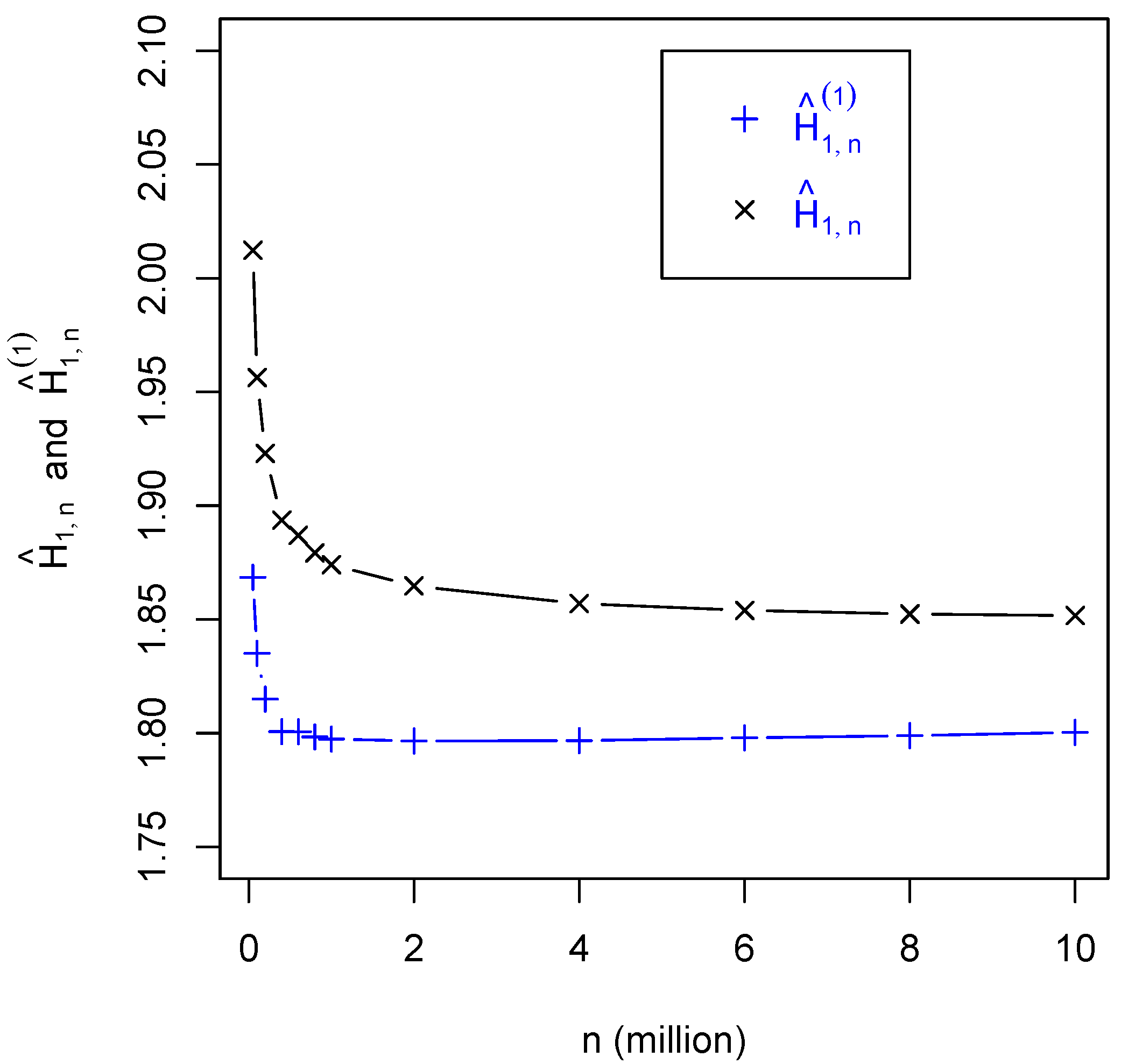
Table 1 presents the circular-distance estimates ${\widehat{H}}_{k,n}^{(1)}$, $k=1,\cdots ,5$ obtained from samples of sizes in the range $n=5\times {10}^4$–$1\times {10}^7$, together with the corresponding Euclidean-distance estimates ${\widehat{H}}_{k,n}$. Figure 1 displays the estimates ${\widehat{H}}_{k=1,n}^{(1)}$ and ${\widehat{H}}_{k=1,n}$ as functions of the sample size n. Noting that the exact entropy value here is, to 4 decimal places, $H=1.8334$, we observe that as n increases the circular-distance estimates initially “undershoot” the exact value and then start to approach it slowly from below. In contrast, the Euclidean-distance estimates approach the exact value monotonically from above. Interestingly, the biases of the two kinds of estimates at sample sizes $n\gtrsim 1$ million are approximately equal in absolute value. The behavior of the circular-distance estimates at $k=2,\cdots ,5$ is similar to that at $k=1$, and the estimate values at different k’s become very close at $n\gtrsim 1$ million.

Figure 1. Plots of the circular- and Euclidean-distance estimates ${\widehat{H}}_{1,n}^{(1)}$ and ${\widehat{H}}_{1,n}$, respectively, as functions of the sample size n, for the analytic distribution of 6 circular variables; the exact entropy value is (to 4 decimals) $H=1.8334$.

To investigate the usefulness of circular-distance NN estimators in the problem of evaluating the configurational entropy of internal rotations in molecules, we used the circular-distance estimator ${\widehat{H}}_{k,n}^{(1)}$ to estimate the entropy of the joint distribution of internal-rotation angles in the molecule of tartaric acid, where the number of variables is $m=7$. Samples of size n up to 14.4 million of the internal-rotation angles were obtained from a molecular dynamics simulation of the (R,S) stereoisomer of this molecule [21]. 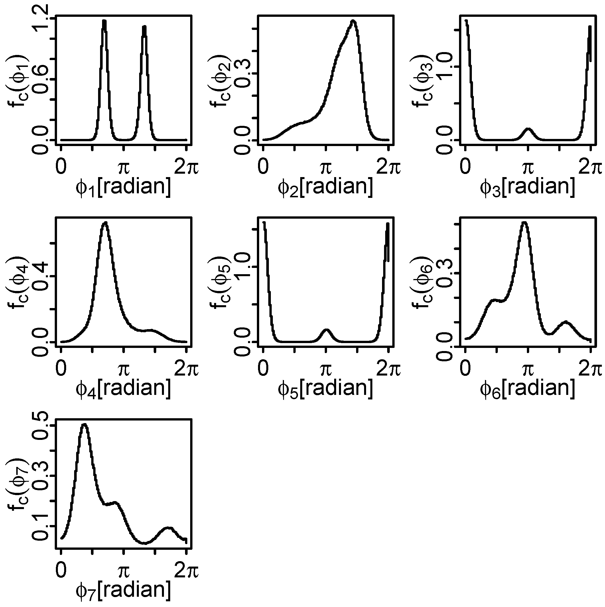Figure 2 shows marginal histograms, smoothed using a Gaussian kernel, of the seven internal-rotation angles of tartaric acid; note that these marginals display markedly non-Gaussian features. The code ANN [22] (with our modification for the circular distance $d_1$), which utilizes a k-d tree algorithm [23], was used for finding the k-th NN distances between sample points. 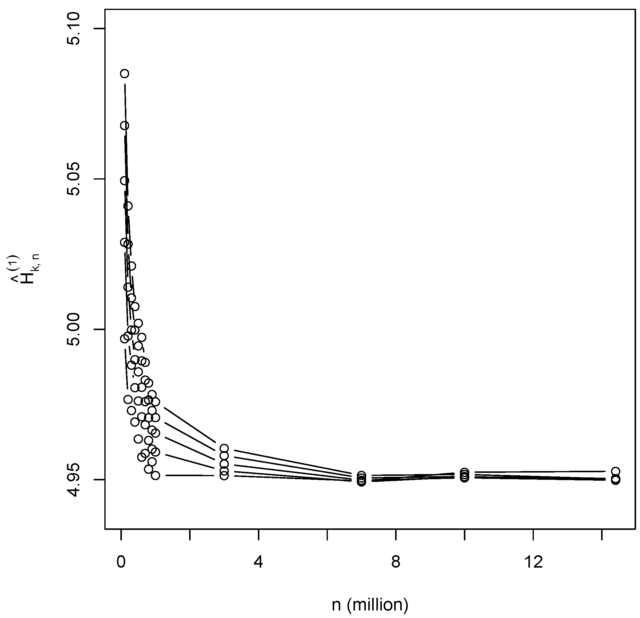Figure 3 presents the estimates ${\widehat{H}}_{k,n}^{(1)}$, $k=1,...,5$ as functions of the sample size n. The values of ${\widehat{H}}_{k,n}^{(1)}$ decrease as n increases, while, at a fixed value of $n\lesssim 7$ million, they increase as k increases; at greater values of n, the estimates at different k’s become quite close in value. 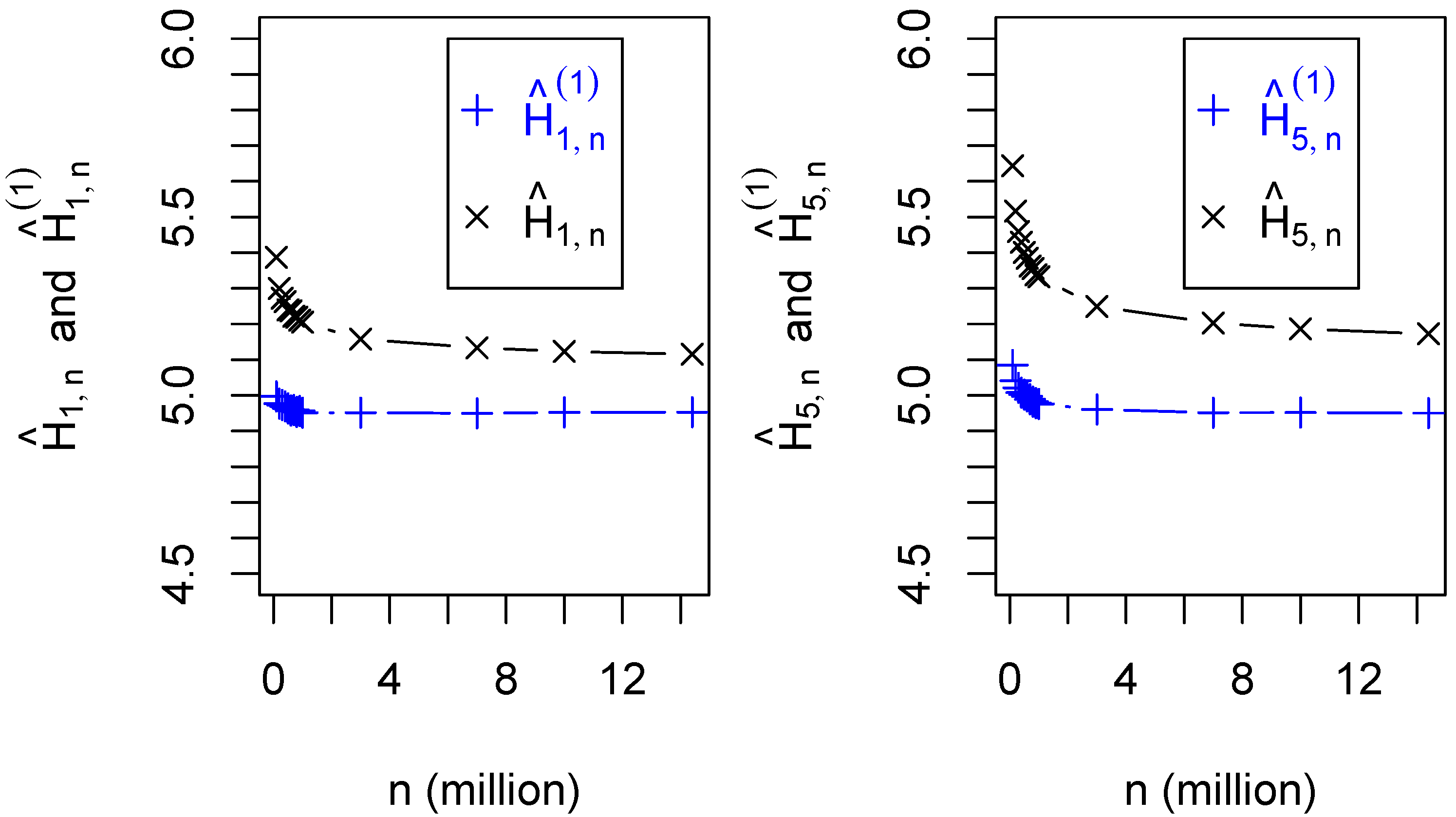Figure 4 compares the circular-distance estimates ${\widehat{H}}_{1,n}^{(1)}$ and ${\widehat{H}}_{5,n}^{(1)}$ with the corresponding Euclidean-distance estimates ${\widehat{H}}_{k,n}$. We note that an $n\to \infty$ extrapolated Euclidean-distance estimate $\widehat{H}=5.04\pm 0.01$ was obtained for this entropy in [21]. Again, as in the case of the analytic circular distribution, this value approximately equals the arithmetic mean of the circular and Euclidean distance estimates at sample sizes $n\gtrsim 1$ million.

Figure 2. Smoothed marginal histograms of the internal-rotation angles ${\varphi }_i$, $i=1,\cdots ,7$ of the (R,S) isomer of tartaric acid obtained by molecular dynamics simulations.

Figure 3. Circular-distance nearest-neighbor estimates ${\widehat{H}}_{k,n}^{(1)}$, $k=1,\cdots ,5$ of the entropy of the 7-dimensional joint distribution of internal-rotation angles in the (R,S) isomer of tartaric acid as functions of the sample size n. The estimates ${\widehat{H}}_{k,n}^{(1)}$ at a fixed $n\lesssim 7$ million increase in value as k increases.

Figure 4. Circular-distance nearest-neighbor estimates ${\widehat{H}}_{1,n}^{(1)}$ and ${\widehat{H}}_{5,n}^{(1)}$ of the internal-rotation entropy of tartaric acid as functions of the sample size n compared with the Euclidean-distance nearest-neighbor estimates ${\widehat{H}}_{1,n}$ and ${\widehat{H}}_{5,n}$. An $n\to \infty$ extrapolated estimate is $\widehat{H}=5.04\pm 0.01$ [21].

Perhaps surprisingly, the results of both the analytic-distribution and molecular-simulation studies undertaken here indicate that only when relatively small data samples are available, the use of a circular-distance estimator has some advantage over the Euclidean-distance estimator. On samples of large size, needed for sufficient convergence of an NN estimate of the entropy of a multivariate distribution, the circular-distance estimates obtained did not have a significantly smaller bias than the Euclidean-distance estimates. In view of such findings, one may question whether the additional computational complexity of a circular-distance estimate is worth the effort. However, we observed that as the sample size increased, the circular NN distances in the sample became quickly so small that the circular-distance estimator ${\widehat{H}}_{k,n}^{(1)}$ coincided in value with the simpler Euclidean-distance estimator ${\widehat{H}}_{k,n}$ in which the same NN-distance values were used. This is explained by the fact that when the circular NN distances $d_1(i,k,n)\le \pi$, the estimator ${\widehat{H}}_{k,n}^{(1)}$ can be replaced with the estimator ${\widehat{H}}_{k,n}$ in which the NN distances $d_1(i,k,n)$ are substituted for the Euclidean NN distances $R(i,k,n)$; this fact follows directly from Remark 2.1 (iii). The only extra computational effort is then expended in finding the circular, instead of Euclidean, NN distances in a given sample.