Turing Systems, Entropy, and Kinetic Models for Self-Healing Surfaces

Department of Industrial Engineering, Tel Aviv University, Ramat Aviv, 69978, Israel
Entropy 2010, 12(3), 554-569; https://doi.org/10.3390/e12030554
Submission received: 30 January 2010
/
Revised: 15 February 2010
/
Accepted: 16 February 2010
/
Published: 15 March 2010
(This article belongs to the Special Issue Entropy and Friction Volume 2)
Abstract
:The paper addresses the methods of description of friction-induced self-healing at the interface between two solid bodies. A macroscopic description of self-healing is based on a Turing system for the transfer of matter that leads to self-organization at the interface in the case of an unstable state. A microscopic description deals with a kinetic model of the process and entropy production during self-organization. The paper provides a brief overview of the Turing system approach and statistical kinetic models. The relation between these methods and the description of the self-healing surfaces is discussed, as well as results of their application. The analytical considerations are illustrated by numerical simulations.
1. Introduction
Self-healing of surfaces is one of the most surprising and complex phenomena of biological systems. It represents spontaneous disappearing of surface defects and restoring initial structure of a surface, and is led and controlled by inner properties of the system. In the last years, self-healing ability of biological systems attracted the attention of material engineers [1,2]. The main goal of engineering studies in this direction is to create artificial systems and surfaces with self-healing properties.
In general, the investigations in the field of artificial self-healing materials design follow two approaches. The first approach addresses design of self-healing materials such that the disappearance of the defects is led by inner abilities of the system and does not require external fields and energy. Such self-healing phenomenon is called autonomic healing, and it is was observed in polymer composites [3,4], including nanocomposites [5], and in the other types of engineered materials [1]. The second approach deals with the systems in which self-healing processes occur under an influence of external fields, while the self-healing process is governed by the system structure and material properties [6,7]. Such phenomenon was considered for polymer materials in thermal fields [8] and for the surfaces in mechanical systems, in which self-healing is induced by friction [2]. The surfaces that have a self-healing property, either without external energy or under the influence of the external fields, are known as self-healing surfaces.
In the last years, a number of methods for modeling and studying of self-healing surfaces both in “microscopic” and in “macroscopic” scales were developed. Design of self-healing polymer composites deals with molecular structures of materials and encapsulated healing agents that started to react with the basic polymer while it was damaged [4]. In contrast, the studies of self-healing in external fields or mechanical influence consider macroscopic models of materials [9] and apply suitable continuity equations for description of self-healing phenomenon on the surfaces. As a result, self-healing is considered as a kind of self-organization phenomenon that leads to the changes of the surface state according to the system properties.
In particular, Gershman and Bushe [10] considered the surfaces with self-healing induced by friction, and suggested to apply the methods that are commonly used for analysis of a self-organization phenomenon (see e.g., [11,12]). They studied self-healing by the use of thermodynamics of non-linear dynamical systems and applied the entropy principles to self-healing [13]. Further progress in this direction was achieved by Nosonovsky and Bhushan [6,7], who considered self-healing as a hierarchical phenomenon. Analysis of this phenomenon by the methods of non-linear dynamical systems theory led to consideration of self-organization that occurs on different hierarchical levels of the material: from nanoscale via microscale to macroscale. Later, Fox-Rabinovich, et al. [14] suggested a criterion that determines the possibility of self-organization on the basis of entropy.
The indicated studies present the entropic concepts and methods for consideration of self-healing by the use of dynamical systems theory. Nevertheless, qualitative or quantitative models that describe the processes on self-healing surfaces in the direct form of self-organizing system have not been reported yet. The objective of this paper is to determine such qualitative models using wide assumptions about the material properties, and to consider its relevance for quantitative analysis of self-healing.
In this paper, self-healing processes on the surfaces are considered using Turing system, which is widely used for modeling and analysis of self-organizing dynamical systems [15,16,17]. A macroscopic behavior of the surface material is modeled by general two components Turing system in two dimensions, while microscopic processes are describes by kinetic equations [13]. Entropy production and occurrence of self-organization on the surface are analyzed by the use of methods and models suggested by Klimontovich [18,19].
In certain cases, analytical considerations of the models are illustrated by numerical simulations.
2. Turing System and Self-Organization Processes
Turing system is a general model that is used for description of the processes in distributed non-linear dynamical systems. This system, also called reaction-diffusion system, was suggested by Turing in 1952 [20] as a method of modeling the processes in distributed chemical media, in which spatial patterns of reagents concentrations can appear. In his initial work, Turing applied this system for description of morphogenesis, while in further decades Turing system was used as a basis for modeling different kinds of non-linear distributed dynamical systems [11,12,17].
In general, Turing system is defined as a following system of n partial differential equations [17]:
where Δ stands for two-dimensional Laplace operator , is interpreted as a vector of reagents concentrations, –as a diffusion matrix. Functions determine behavior of reagents and their relations, and υ stands for bifurcation parameter. It is assumed that the system is defined on a certain domain and that initial and boundary conditions are determined, as well.
In the case of linear functions , behavior of the system is rather simple. For example, let us consider system (1) that describes a media that consists of connected oscillators [21]. In this case, and the system is written as follows:
where and are diffusion coefficients for reagents and , respectively, and is a frequency of oscillations. Indeed, if , then system (2) can be transformed to the equation that describes a linear oscillator without dissipation.
If, in opposite, functions in system (1) are non-linear, then the system can demonstrate different types of behavior. For such a system there exists a value of parameter υ such that if , then homogeneous state of the media is unstable, and the system behaves as follows [22]:
- −
- if then a short external influence on the system gives a rise to static or pulse auto-waves;
- −
- if then auto-waves and wave structures appear without external influence.
Wave structures that appear in the system are known as dissipative structures and also called Turing structures or Turing patterns. In special cases, system (1) has also solitary solutions that represent single running or static pulse-waves over a homogeneous media.
To illustrate a behavior of the media that is described by system (1), let us consider an example of Turing patterns formation the surface of semiconductor plate [23,24,25]. In this example, and represent non-stable concentrations of electrons and holes. In this case, the Turing system has the following form:
In such a two-component system, auto-waves can exist if and , and dissipative structures can appear if [17]. Assume that these requirements hold true, and that functions and correspond to quadric recombination:
where , and , are positive constants and , determine stationary concentrations.
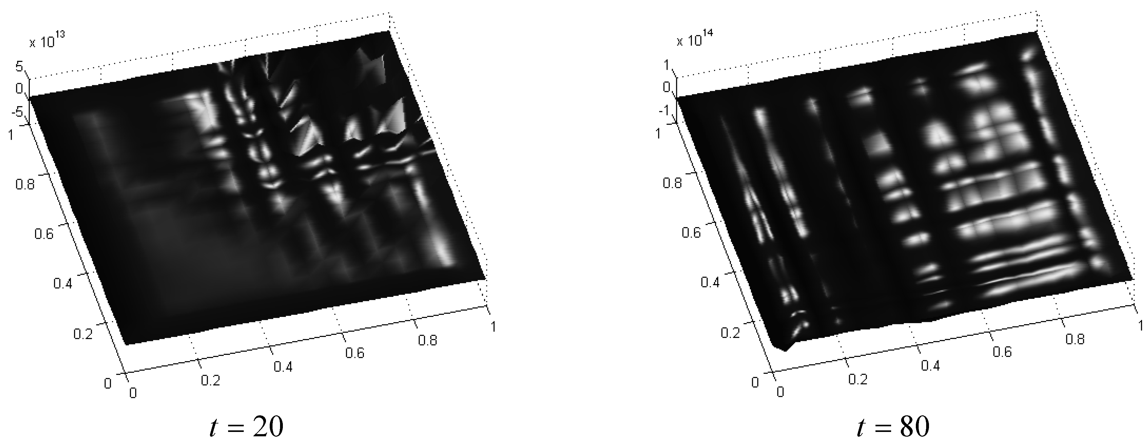
A direct numerical simulation of system (3) for parameters of silicon , , , , shows that on initially homogeneous surface appear running waves and the system does not converge to some steady state. In the simulations, it was assumed that the system starts from the state , , and that at the bounds and are equivalent to zero. The results of simulations are illustrated by Figure 1.
Figure 1.
Results of numerical simulation of system (3) with parameters of silicon.

However, for parameters of the system , , , , that correspond to germanium, numerical simulation demonstrate its fast convergence to the stable state. Such a behavior clarifies the reason of less noise as it is demonstrated by germanium electronic devices comparatively to silicon devices.
In certain cases of engineered systems, system (1) can include both concentrations of reagents and velocities of their production that allows to control patterns formation. For example, Balkarey, et al. [26,27] implemented such approach for design of self-organizing systems of information storage. The model for a two-layer system of distributed Van-der-Pol equations has the following form [26]:
where and , similar to variable in system (2), have a meaning of velocities of and . Coefficients , , determine connection between the layers, and coefficients , , , determine relation between the frequencies within the layers. In this system, stable Turing patterns exist [26,27], and their formation can be controlled both by boundary conditions [25] and by distributed external field [23,24].
As indicated above, Turing systems (1) with non-linear functions allow the processes of self-organization that, according to definition of the system, occur on the surface of the described system. These processes are represented by appearance of spatial running or stable wave structures. Recently, Leppänen presented a number of numerical examples of such structures for different Turing systems [28,29] and also reported about existence of stable three-dimensional Turing patterns. In this case, Laplace operator Δ in system (1) has a three-dimensional form, , indeed, and functions f depend on first spatial derivations of u. Last years, similar results were obtained by Shoji, et al. [30], and stable solitary solutions in three-dimensional Turing systems were obtained in the field of non-linear optics [31].
3. Kinetic Models and Entropy
In the above-presented Turing system (1), values , , were interpreted as reagents concentrations or other macroscopic measures that can be obtained by direct observation. Now let us consider a kinetic representation for such systems.
3.1. Concentrated Turing System
Let us start with a concentrated Turing system and as an example let us consider a Van-der-Pol equation, as it was studied by Klimontovich [18,19]:
In the form of concentrated Turing system is can be written as follows [19]:
where stands for the energy of oscillations with frequency ω and ; is a parameter that represents a feedback and represents a value of linear energy dissipation. System (5) is a kind of system (1) that can be considered as a description of behavior of each element in the distributed system of non-interacting oscillators.
In spite of the existence of the exact solution of system (5), let us consider a distribution μ of oscillations energy E. This distribution is presented by a Fokker-Planck equation for system (5) that has the following form [19]:
where δ stands for intensity of external source of fluctuations. If fluctuations depend on the energy of oscillations and do not depend on external sources, as it holds, e.g., for quantum oscillators, then and system (6) has a form
where k stands for Boltzmann constant and T has a meaning of temperature for the oscillations with frequency ω.
Stationary solution of system (6) is given by the Gibbs distribution [19,32]:
where H is a Hamilton function and stands for free energy. The Shannon entropy of distribution is given by a formula:
Regarding parameter , there exist three cases that, according to formulas (8) and (9), give the following distributions μ, entropies S and average energies [19,32]:
- Chaotic behavior that holds while and . Then
- Threshold state with . Then
- Generating regime while and . Then
For these three cases, it holds true that while . A renormalization of entropies S using average energies gives the following values of fluctuations:
and the following renormalized entropies :
For the renormalized entropies , it holds true that , i.e., while a value of control parameter increases, its system entropy renormalized by the average energy decreases, which represents occurrence of self-organization process in the system. The self-organization in the considered systems means that it moves from chaotic behavior (case 1) via threshold state (case 2) to generating regime (case 3). This statement is known as Klimontovich S-theorem [19,32] that gives a quantitative criterion of self-organization occurrence similar to the value of bifurcation parameter υ in system (1). In the considered example of Van-der-Pol equation, bifurcation parameter υ corresponds to and its bifurcation value is . In addition, the construction required by S-theorem demonstrates a correspondence between macroscale description (5) and microscale description (6) of system behavior in the terms of energy distributions.
3.2. Distributed Turing System
Let us apply the above presented approach to the distributed Turing system (1). In such system, concentrations , , depend on spatial coordinates, in the considered two-dimensional case – on x and y coordinates. Hence, distribution μ of energy E for distributed Turing system is also a two-dimensional function that is normalized over time and spatial coordinates.
In system (1), generating regime depend both on inner energy of oscillations and on spatial diffusion D. Hence, kinetic Fokker-Planck equation (7) for distribution μ obtains the following form:
where F is a function that corresponds to the functions f in system (1). In particular, for distributed system of Van-der-Pol oscillators (5), equation (10) is similar to equation (7) with an addendum that relates to the spatial diffusion [19]:
The last equation was studied by Klimontovich [18,19], and it was found that the number N of distributed oscillators with distribution (11) plays the same role as a bifurcation parameter υ for the system. The above-mentioned two-layer system (4) provides an example of such system with . In certain sense, these results correspond with the Fox-Rabinovich, et al. consideration [14] of self-organization criterions.
Since distribution μ depends on spatial coordinates x and y, energy E can be considered as a function of x and y. Then Fokker-Planck equation (10) for distribution μ can be written in a general form as follows [33]:
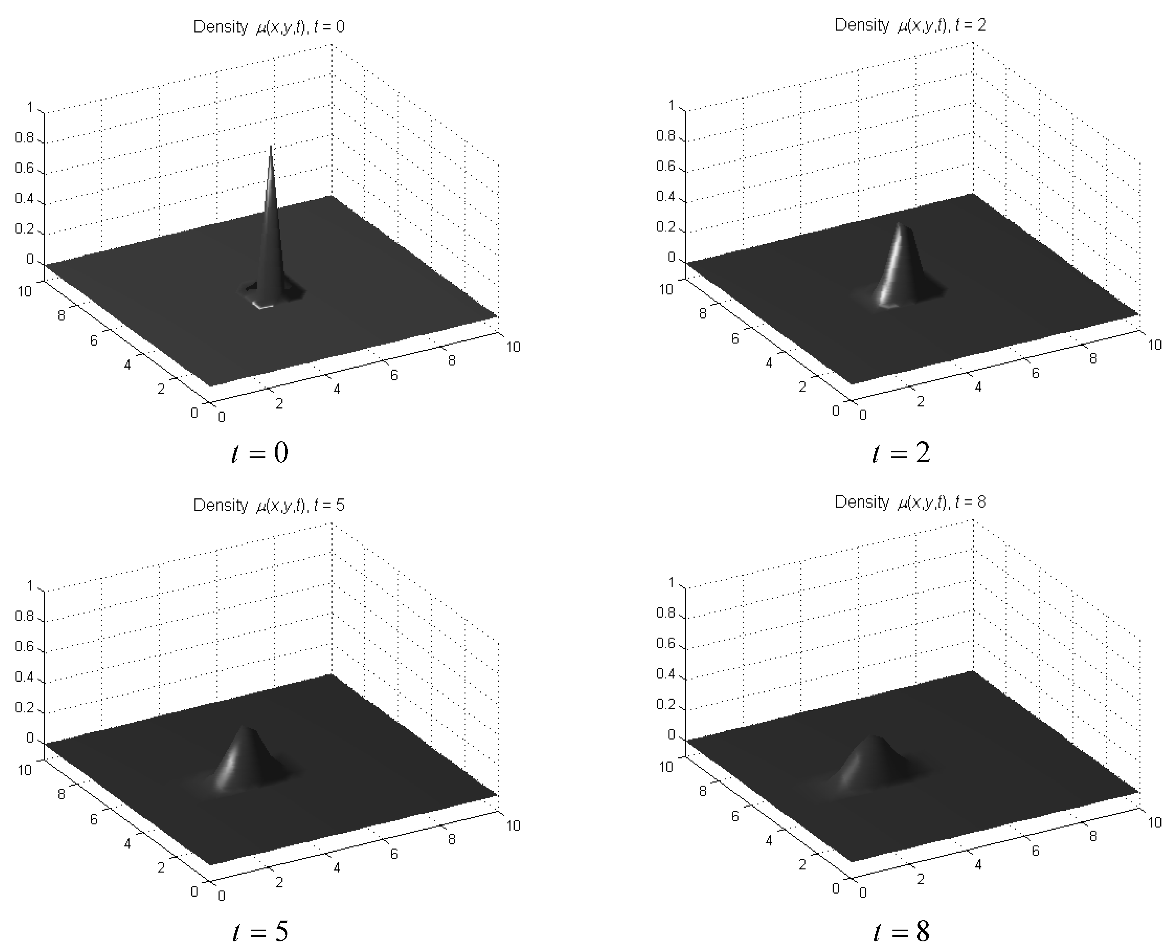
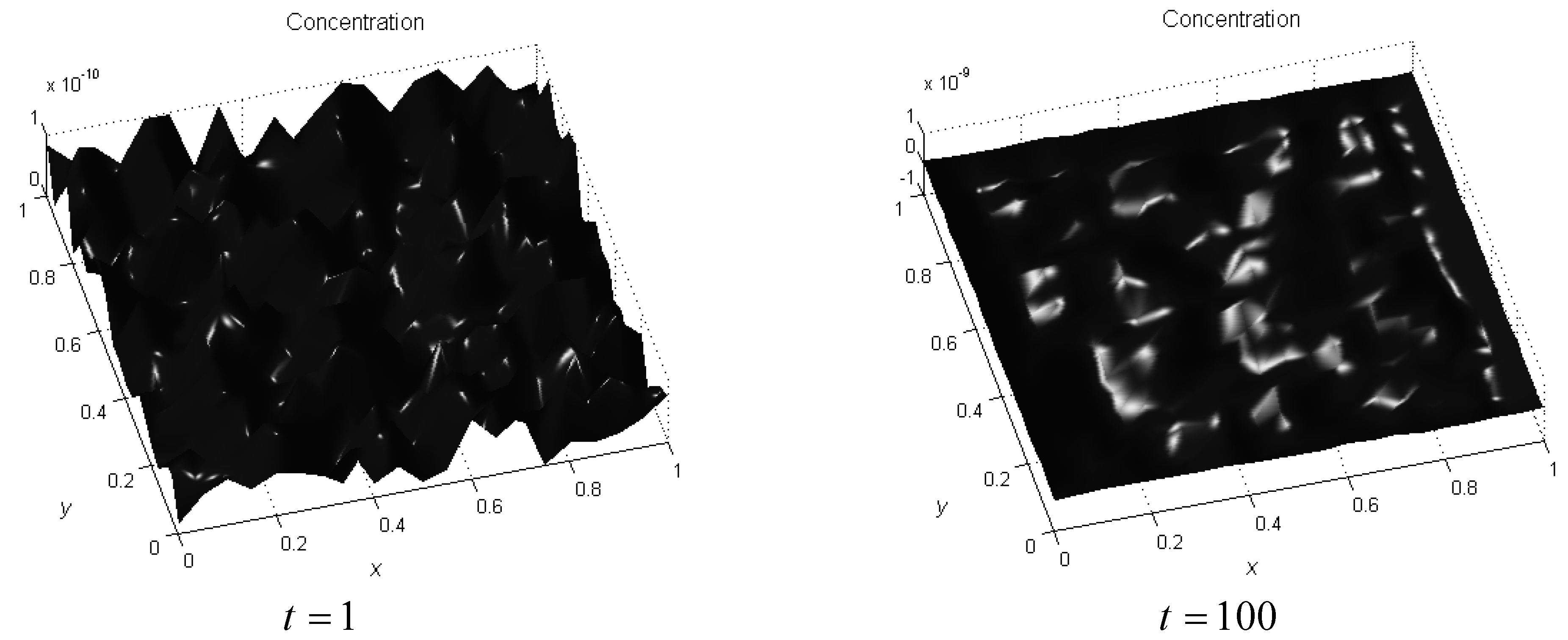
where and , , are some functions that correspond to the functions of considered system (1) and that in liner case do not depend on distribution μ [34]. As above, in equation (12) indexed α-s correspond to diffusion effects, while their formal definition differs from their definition in systems (2) and (3). An example of density dynamics for equation (12) with constant coefficients , , and is shown in Figure 2. The figure is obtained by direct numerical simulation of equation (12) over square domain with zero boundary conditions. The steps in spatial coordinates x and y are equivalent to , and the step in time coordinate is equivalent to 1. Initial state is presented by symmetric two-dimensional Gaussian distribution with that is concentrated in the center of the domain.
Figure 2.
Example of density dynamics for equation (12) with constant coefficients.

As in the above-considered example of Van-der-Pol equation, Turing system (1) and Fokker-Planck equations (10) or (12) present two forms of system description: the first deals with a description in the terms of concentrations and the second – with density. Thus, it can be expected that for these equations the consideration of entropy as some criterion of self-organization can be useful as well.
In general, kinetic equations (10) and (12) that corresponds to the system (1) cannot be solved analytically. Nevertheless, an application of entropic measures as measure functions and consideration of the equations stability relatively to those measures can provide criteria of self-organization occurrence.
We will follow the above-considered approach that is based on Shannon entropy for equation (10). The considerations of equation (12), which in addition to Shannon entropy include Renyi and Tsalis entropies, are presented by Frank [33]. In the implementation of entropic measures as measure functions we follow a direction that was suggested by Klimontovich [19], while in details of the methods for studies of distributed systems stability relatively to measure we follow an approach presented by Sirazetdinov [35].
Similar to formula (9), the Shannon entropy of distribution μ that is governed by equation (10) is defined as follows:
In addition, we will use a Kullback-Leibler distance, also called Boltzmann-Kullback measure [33], that determines the distance between distribution for an energy E and distribution :
where stands for such energy that the entropy in the sense of equation (10) reaches its maximum.
Notice that both E and are functions of coordinates x and y, and distribution corresponds to uniform distribution that, according to maximum of entropy, represents a chaotic regime of the system. Such understanding of chaotic regime in distributed systems differs from the understanding of chaotic behavior in concentrated systems. In fact, in concentrated systems, stable homogeneous movement corresponds to regular behavior, while in distributed systems a uniform spatial distribution means the most non-regular concentrations of reagents.
Kullback-Leibler distance (14) meets the required properties of a processes measure function [35]:
- −
- for any time-moment t,
- −
- , that follows form conventional assumption that ,
- −
- for any μ, Kullback-Leibler distance is continuous in time, that follows from continuality of distribution μ and energy E.
It is easy to certify that the entropy (13) can be considered as a positive functional [35] relatively to Kullback-Leibler distance. According to the assumption about , it is strictly positive. Hence, distance is bounded with a finite upper bound. From general properties of entropy for any distribution μ and by the same convention that .
Now we are ready to apply a theorem on instability of steady processes [35] that, in the introduced terms, states that if then distribution μ is unstable relatively to distance . In the light of above-considered Klimontovich’s S-theorem [19,32], this theorem is intuitively obvious, since it states that distribution μ becomes non-uniform if its entropy decreases from its maximum that is reached for uniform distribution. The simple meaning of the theorem allows certain quantitative description of the system behavior. By the use of the entropy definition (13), we obtain:
Since for any x and y, the first addendum is positive, while the second addendum is negative. Hence the sign of is determined by the values of that are defined by distribution μ and by the values of .
If then and the state with uniform distribution is stable. However, already for distribution μ such that its dependence on E and t is given by a formula:
where is a normalization coefficient with the meaning of steady state energy, function is harmonic and proportional to (a strict formula for the function is rather complex and we omit it here). Thus, periodically becomes negative or positive; while it is negative, distribution μ changes, and while it is positive, distribution μ stays unchanged. Such behavior corresponds to appearance of running waves that are similar to the waves in the above-presented example of Turing system (3).
The consideration of entropy changing in time can allow certain description of self-organization in distributed Turing systems. Nevertheless, because of the complexity of required calculations it can be applied for relatively simple systems. Additional information about self-organization and its relation with the entropy may be obtained by consideration of two Kolmogorov equations. The first equation is equivalent to the Fokker-Planck equation, while the second governs transitions between the states. Such representation requires further consideration of the system behavior on microscale level. Some possible techniques for such considerations are presented by Klimontovich [18,19] and Landa [21]. Below, we will give some remarks on such techniques.
4. Remarks on Wave Behavior
As indicated above, analysis of the system behavior at microscale level requires additional techniques and methods. Let us consider a possible way of modeling such behavior as it is presented by Landa [21]. In particular, let us consider a non-linear Ginzburd-Landau equation that for (2+1)-dimensions has the following form:
where . If shift velocity over y is equivalent zero then this equation obtains a form of standard time-dependent Ginzburg-Landau equation:
that in the running with velocity coordinates is a cubical Schrödinger equation:
In the case of two-dimensional operator Δ, this equation describes behavior of wave pulses on the surface with spatial x and y coordinates.
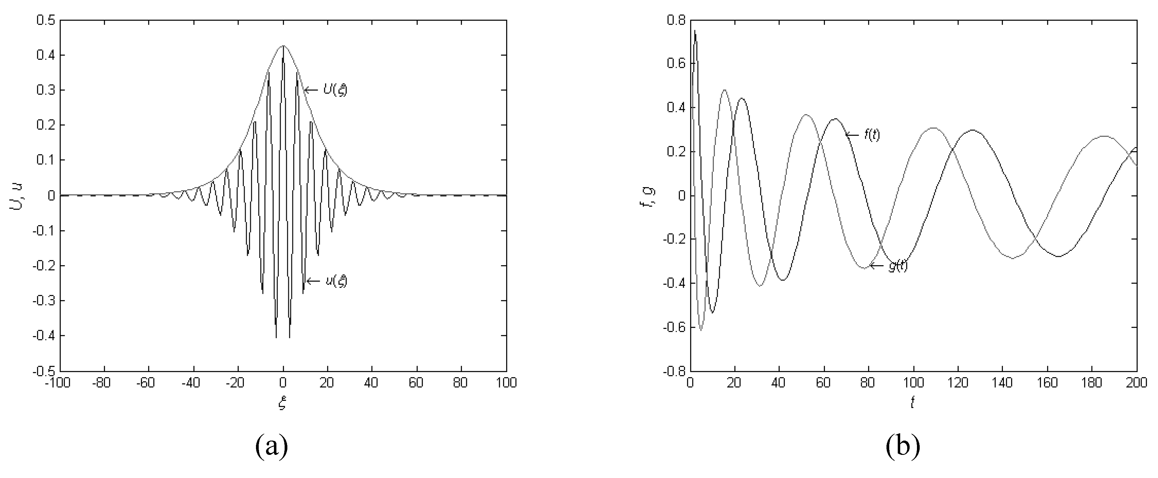
Cubical Schrödinger equation (16) allows a number of solution types. Solutions in the form of stable and running waves are similar to the waves shown in Figure 1. In addition, this equation allows a solitary solution that for (1+1)-dimensional equation (16) has a form [21]:
and is illustrated by Figure 3.a.
Equation (16) is written in a complex form while in the form of two real equation it can be represented by a Turing system (1) as follows [21]. Let , where f and g, as well as u, are functions of spatial coordinates and time. Then equation (16) obtains a form of the following system:
where function f can be corresponded to a birth density and function g – to a death density. Behavior of these functions is illustrated by Figure 3.b.
Figure 3.
(a) Solitary solution of cubical Schrödinger equation (16) in (1+1)-dimensions. (b) Birth f and death g densities for system (17) corresponding to equation (16).
Figure 3.
(a) Solitary solution of cubical Schrödinger equation (16) in (1+1)-dimensions. (b) Birth f and death g densities for system (17) corresponding to equation (16).
Each of two equations of system (17) is a nonlinear Fokker-Planck equation that describes a behavior of the Brown particle in the external field such that its behavior depends on previous states. Notice that in system (17) the first equation does not include and the second equation does not include , i.e., as it follows from quantum mechanical nature of equation (16), spatial behavior of reagents depends on the behavior of each other but does not depend on the reagent behavior itself. In the description that includes both macroscale and microscale levels, each equation of system (17) have to include both and with suitable coefficients. Nevertheless, analysis of such system is rather complex and remains to future research.
5. Friction-Inspired Self-Organization on Surfaces
Let us implement the above-presented models to the contact surfaces of solid bodies during friction. The goal of the next consideration is to give additional illustration of Turing system behavior and to introduce such models into the context of self-healing during friction. We consider the simplest case of friction of solid bodies without lubrication. For further information on friction and methods of its studies see books [36,37], and for consideration of self-organization during friction see monographs [2,6].
Assume that there are two solid bodies that contact by their surfaces and that one the bodies is moving relatively to the other. Since the contact surfaces have microdefects, the surfaces are rough and, under certain pressure, abrasion occurs. That leads to flattening of the contact surfaces, while a near-surface structure of the material is disturbed. This process is followed by heating of the bodies and by the changes in their electric charges; that in their turn lead to the non-zero flows of the matter in near-surface layers. Schematic illustration of the considered process is shown in Figure 4; this figure is based on an illustration presented by Garkunov [37].
Figure 4.
Scheme of two solid bodies and their contact surfaces (based on [37]).
Figure 4.
Scheme of two solid bodies and their contact surfaces (based on [37]).
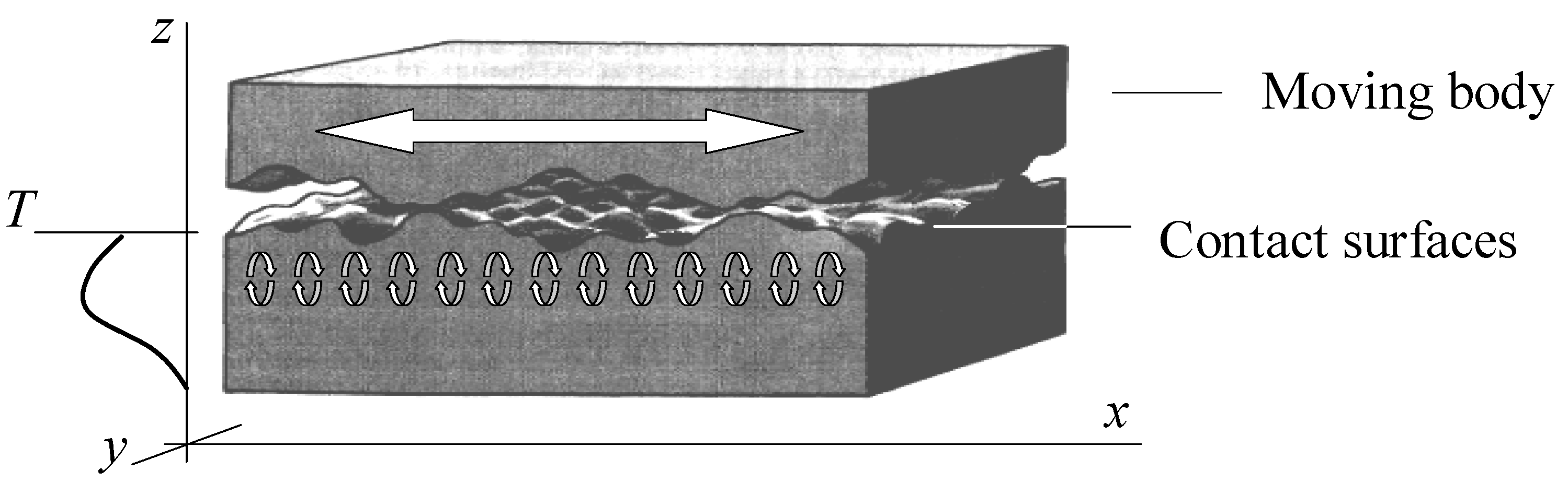
In Figure 4, the bottom body stays still and the upper body moves over the x axis. It is assumed that the pressure is applied to the upper body and is directed down over the z axis. In addition, the Figure shows a near-surface matter flows and a distribution of temperature T in the bottom body [37].
As indicated above, at least three processes govern matter concentrations on the contact surfaces: heat flow and corresponding matter flow, abrasion and corresponding changes of matter concentration and changes of electric charges of the bodies and corresponding flow of ions. From the macroscale point of view, we are interested in first two processes.
Let us formulate a Turing system that describes these processes. In this formulation, we follow the considerations of one-dimensional heat and matter flows that are presented by Berkovich and Gromakovsky [36] and by Garkunov [37], and distribute these considerations to the three-dimensional case. We apply normalized units for temperature and for matter concentration , and consider the processes in the bottom body (see Figure 4).
An implementation of one-dimensional equation for a heat flow [37] to the three-dimensional case with abrasion gives the following equation:
where represents a diffusion of temperature over a surface; corresponds to the diffusion and heat flow via the surface, where function determines a proportional dependence of on the heat flow and opposite dependence on matter concentration ; and function (also called heat ejection [37]) takes into account an abrasion that decreases concentration and effects of temperature changes during friction.
Formulation of equation for matter concentration on a surface is based on the Fick diffusion equations [38] and takes into account a matter flow over the z axis [36]. The equation is formulated as follows:
where represents a diffusion of matter on a surface; corresponds to the matter flow via the surface because of abrasion, where function determines a proportional dependence of on the matter flow from the body because of temperature and electric charge effects and opposite dependence on matter concentration ; and function takes into account a dependence of abrasion on temperature .
Equations (18)-(19) form a Turing system that in the case of non-linear functions α, δ and ω allows a self-organization on a contact surface. Strict solutions of equations (18)-(19) can be obtained in special cases of these functions, however, effects of self-organization can be observed by numerical simulations. In Figure 5, we present results of such simulations for constant diffusion coefficients α, , , and , where .
Figure 5.
Results of numerical simulation of system (18)–(19) with modeling parameters.
From Figure 5, it follows that initially random defects of surface are flattening out with time, while the concentration of the matter at the contact surface increases. During the simulations, it was observed that the concentration changes periodically and moves to steady oscillating over the surface. Nevertheless, notice again that the simulations were conducted for modeling parameters, while consideration of the processes for real materials requires additional research.
6. Conclusion
In the paper, we considered some models that can be applied for description and modeling of self-healing surfaces, in particular, of contact surfaces during friction. For modeling of self-healing surfaces, Turing systems are considered and their behavior is analyzed.
It is demonstrated that known entropy methods of self-organization analysis naturally correspond to the models based on Turing systems. Moreover, in the case of distributed systems, Turing system can be considered as a suitable model both for dynamics of reagent concentrations (macroscale level) and for dynamics of matter distribution (microscale level). This fact, in addition to correspondence of Turing systems with entropy methods, makes such models r useful in the description of self-healing surfaces.
In this paper, macroscale Turing system that describes dynamics of matter distribution was analyzed by the use of methods of stability by measure, while measure functions were determined by entropy measures. This analysis demonstrated an application of entropy criteria of self-organization to Turing systems. Nevertheless, this consideration showed that the quantitative consideration of distributed self-organizing systems by the use of entropy methods is rather complex and can be applied for relatively simple systems.
Regarding a microscale level, it was demonstrated that the known quantum-mechanical non-linear models can be considered as a kind of Turing systems. By adding suitable diffusion coefficients, such models can be applied for friction analysis both at microscale and at nanoscale levels. In addition, such approach provides a wide context for friction analysis and relates its studies with probabilistic and quantum-mechanical models.
Finally, the paper presents an illustrative example of description of self-healing during simple friction. For contact surfaces of solid bodies, a modeling Turing system is formulated, and its behavior is considered by direct numerical simulations. It is demonstrated that for certain modeling parameters, the system allows a process of self-healing on the contact surface. The further consideration of such models and their application to certain materials and friction conditions is remains for further research.
Acknowledgements
I am grateful to V. P. Rijov for numerous discussions on self-organization and entropy of dynamical systems, to M. Nosonovsky who introduced me into the field of self-healing surfaces and materials, and to B. Golani, A. Gruber, S. Hodorov, S. Kann and V. Segal and for their stimulating interest to the described models.
References
- Van der Zwaag, S. (Ed.) Self Healing Materials. An Alternative Approach to 20 Centuries of Materials Science; Springer-Verlag: Dordrecht, Netherlands, 2007.
- Fox-Rabinovich, G.S.; Totten, G.E. (Eds.) Self-Organization During Friction. Advanced Surface-Engineered Materials and Systems Design; Taylor & Francis: Boca Raton, FL, USA, 2007.
- Hayes, S.A.; Zhang, W.; Branthwaite, M.; Jones, F.R. Self-healing of damage in fibre-reinforces polymer-matrix composites. J. R. Soc. Interface 2007, 4, 381–387. [Google Scholar] [CrossRef] [PubMed]
- White, S.R.; Sottos, N.R.; Geubelle, P.H.; Moore, J.S.; Kessler, M.R.; Sriram, S.R.; Brown, E.N.; Viswanathan, S. Autonomic healing of polymer surfaces. Nature 2001, 409, 794–797. [Google Scholar] [CrossRef] [PubMed]
- Balazs, A.C. Modeling self-healing materials. Materials Today 2007, 10, 18–23. [Google Scholar] [CrossRef]
- Nosonovsky, M.; Bhushan, B. Multiscale Dissipative Mechanisms and Hierarchical Surfaces; Springer-Verlag: Berlin, Heidelberg, 2008. [Google Scholar]
- Nosonovsky, M.; Bhushan, B. Thermodynamics of surface degradation, self-organization and self-healing for biomimetic surfaces. Phil. Trans. R. Soc. A 2009, 367, 1607–1627. [Google Scholar] [CrossRef] [PubMed]
- Varley, R.J.; Zwaag, S.van der. Towards an understanding of thermally activated self-healing of an ionomer system during ballistic penetration. Acta Materialia 2008, 56, 5737–5750. [Google Scholar]
- Gerde, E.; Marder, M. Friction and fracture. Nature 2001, 413, 285–288. [Google Scholar] [CrossRef] [PubMed]
- Gershman, I.S.; Bushe, N.A. Elements of thermodynamics and self-organization during friction. In Self-Organization during Frict; Fox-Rabinovich, G.S., Totten, G.E., Eds.; Taylor & Francis: Boca Raton, FL, USA, 2007; Chapter 2; pp. 13–56. [Google Scholar]
- Haken, H. Synergetics. An Introduction. Nonequilibrium Phase Transitions in Physics, Chemistry and Biology, 3rd ed.; Springer-Verlag: New York, NY, USA, 1983. [Google Scholar]
- Nikolis, G.; Prigogine, I. Self-Organization in Nonequilibrium Systems; John Willey & Sons: New York, NY, USA, 1977. [Google Scholar]
- Prigogine, I. Thermodynamics of Irreversible Processes; John Willey & Sons: New York, NY, USA, 1968. [Google Scholar]
- Fox-Rabinovich, G.; Gershman, I.S.; Yamamoto, K.; Veldhuis, S.; Agguire, M.; Beake, B.; Kovalev, A.; Biksa, A. Self-organization during friction in complex surface engineered tribo-systems. Entropy 2010, 12, 275–288. [Google Scholar] [CrossRef]
- Gaponov-Grekhov, A.V.; Rabinovich, M.I. Auto-structures. Chaotic dynamics of ensembles. In Non-linear Waves. Structures and Bifurcations; Gaponov-Grekhov, A.V., Rabinovich, M.I., Eds.; Nauka: Moscow, Russia, 1987; pp. 7–44. [Google Scholar]
- Gaponov-Grekhov, A.V.; Lomov, A.S.; Osipov, G.V.; Rabinovich, M.I. Creation and dynamics of two-dimensional structures in non-stable dissipative medias. In Non-linear Waves. Structures and Bifurcations; Gaponov-Grekhov, A.V., Rabinovich, M.I., Eds.; Nauka: Moscow, Russia, 1988; pp. 61–83. [Google Scholar]
- Vasiliev, V.A.; Romanovskii, Yu.M.; Chernavskii, D.S.; Yakhno, V.G. Auto-wave Processes in Kinetic Systems: Spatial and Temporal Self-organization in Physics, Chemistry, Biology, and Medicine; D. Reidel Publishing Company: Dordrecht, The Netherlands, 1987. [Google Scholar]
- Klimontovich, Yu.L. Problems in the statistical theory of open systems: criteria for the relative degree of order in self-organization processes. Sov. Phys. Usp. 1989, 32, 416–433. [Google Scholar] [CrossRef]
- Klimontovich, Yu.L. Turbulent Motion and the Structure of Chaos; Kluwer Academic Publishers: New York, NY, USA, 1991. [Google Scholar]
- Turing, A.M. The chemical basis of morphogenesis. Phil. Trans. R. Soc. B 1952, 237, 37–72. [Google Scholar] [CrossRef]
- Landa, P.S. Nonlinear Oscillations and Waves in Dynamical Systems; Kluwer Academic Publishers: Dordrecht, Boston, London, 1996. [Google Scholar]
- Kerner, B.S.; Osipov, V.V. Autosolitons. Uspehi Fiz. Nauk 1989, 157, 201–206. [Google Scholar] [CrossRef]
- Kagan, E. A Model of concentration structures on the semiconductor’s surface. Izvestiya TREI 1995, 1, 43–45. [Google Scholar]
- Kagan, E. On the realization of controlled patterns’ formation on the semiconductor surface. In Proceedings of the Third International Arctic Seminar on Physics and Mathematics IAS’98, Murmansk State Pedagoical University, Murmansk, Russia, 1998; pp. 48–51.
- Kagan, E. Stability of turing patterns in a reaction-diffusion system with boundary control. In Nanomaterials: Methods and Approaches; Belonenko, M.B., Ed.; PrinTerra: Volgograd, Russia, 2008; pp. 134–147. [Google Scholar]
- Balkarey, Yu.I.; Elinson, M.I.; Evtikhov, M.G. Auto-waves and dissipative structures in two-layers medium of Van der Pol Oscillators connected by diffusion. J. Theor. Phys. 1987, 57, 209–218. [Google Scholar]
- Balkarey, Yu.I.; Elinson, M.I.; Evtikhov, M.G. Auto-waves, Dissipative structures and storing information in multi-layers medium with diffusion. Microelectronics 1988, 17, 313–320. [Google Scholar]
- Leppänen, T. Computational Studies of Pattern Formation in Turing Systems. PhD Dissertation, Helsinki University of Technology, Espoo, Finland, 2004. [Google Scholar]
- Leppänen, T. The theory of turing pattern formation. In Current Topics in Physics; Kaski, K., Bario, R.A., Eds.; Imperial College Press: London, UK, 2005; pp. 190–227. [Google Scholar]
- Shoji, H.; Yamada, K.; Ueyama, D.; Ohta, T. Turing patterns in three dimensions. Phys. Rev. E 2007, 75, 046212. [Google Scholar] [CrossRef] [Green Version]
- Mihalache, D.; Mazilu, D.; Lederer, F.; Malomed, B.A.; Crasovan, L.-C.; Kartashov, Y.V.; Torner, L. Stable Three-dimensional solitons in Attractive Bose-Einstein Condensates loaded in an optical lattice. Phys. Rev. A 2005, 021601(R). [Google Scholar] [CrossRef]
- Klimontovich, Yu.L. Entropy evolution in self-organization processes H-theorem and S-theorem. Physica A 1987, 142, 390–404. [Google Scholar] [CrossRef]
- Frank, T.D. Nonlinear Fokker-Planck Equations. Fundamentals and Applications; Springer-Verlag: Berlin, Germany, 2005. [Google Scholar]
- Risken, H. The Fokker-Planck Equation. Methods of Solution and Applications; Springer-Verlag: Berlin, Germany, 1989. [Google Scholar]
- Sirazetdinov, T.K. Stability of Distributed Systems; Nauka: Novosibirsk, Russia, 1987. [Google Scholar]
- Berkovich, I.I.; Gromakovsky, D.G. Tribology; Samara State University of Technology Press: Samara, Russia, 2000. [Google Scholar]
- Garkunov, D.N. Triboengineering (Wear and Non-Wear); Moscow Agricultural Academy Press: Moscow, Russia, 2000. [Google Scholar]
- Armazov, B.N.; Mukhina, G.G. (Eds.) Materials Theory; Moscow State Technical University (MSTU n. a. N. E. Bauman) Press: Moscow, Russia, 2005.
© 2010 by the authors; licensee Molecular Diversity Preservation International, Basel, Switzerland. This article is an open-access article distributed under the terms and conditions of the Creative Commons Attribution license (http://creativecommons.org/licenses/by/3.0/).
Share and Cite
MDPI and ACS Style
Kagan, E. Turing Systems, Entropy, and Kinetic Models for Self-Healing Surfaces. Entropy 2010, 12, 554-569. https://doi.org/10.3390/e12030554
AMA Style
Kagan E. Turing Systems, Entropy, and Kinetic Models for Self-Healing Surfaces. Entropy. 2010; 12(3):554-569. https://doi.org/10.3390/e12030554
Chicago/Turabian StyleKagan, Eugene. 2010. "Turing Systems, Entropy, and Kinetic Models for Self-Healing Surfaces" Entropy 12, no. 3: 554-569. https://doi.org/10.3390/e12030554