1. Introduction
Time series analysis is not only a very important technique for identifying different components and revealing variation characters of the variable studied, but also is the basis of many simulation and forecast works, thus it has been widely used in many different fields of applied researches and engineering practical works presently, such as electronics, business, medicine, physics, earth sciences, hydraulic engineering and among others [
1,
2,
3,
4,
5,
6,
7,
8]. However, due to the influence of many random and uncertain natural factors as well as the subjective factors, observed time series data always include many noises, which contaminate the real series data and cause many difficulties in the time series data analysis process, e.g., periods’ identification, parameters’ estimation, simulation and forecasting,
etc. [
9,
10,
11,
12,
13,
14]. Due to the existence of noises, it is not an easy task to get accurate time series analysis results in practical works. As far as the noises are concerned, they are generally classified as either additive or dynamical, and additive noises are sometimes called measurement noises [
15,
16]. Comparatively, the dynamical noises are generated by certain physical mechanisms, so they usually show good correlations (or maybe constants sometimes) and can be identified and modified easily; but the additive noises often show random characters and are difficult to be analyzed and described accurately. In the present paper, on the basis of the different physical generation mechanisms between real series and noises in observed time series data [
15], the components which have pure random characters and are generated by random and uncertain factors are defined as noises, and they are the main focus to be studied in this paper.
In order to obtain accurate and reliable time series data analysis results in practical works, noises reduction or removing should precede other tasks in the time series analysis process. At present, there have been a number of de-noising methods. Among them, one kind of de-noising methods is to establish suitable deterministic models to simulate the observed time series first, and then regard the difference between observed series and simulated series as noises [
17,
18]. However, many real natural evolution mechanisms cannot be understood completely now and sometimes even know nothing, so the real models are unknown in these cases and the de-noising results are unreliable. Another important kind of de-noising methods is based on spectral analysis [
19]. Since most of time series in nature show many complex variation characters [
20,
21,
22] (e.g., the hydrologic time series are the most representative because of usually showing extremely non-stationary and nonlinear characters which result from spatial and dynamical heterogeneities and also showing multi-temporal scale variation characters [
9,
23,
24], so they will be the examples in “cases studies” in
section 5), these traditional spectral analysis-based methods (Wiener filtering, Kalman filtering, Fourier transform and among others) have many disadvantages and also cannot meet the practical needs enough. For examples, Wiener filtering method and Kalman filtering method are only suitable for linear natural systems, and the analysis results depend on the establishment of state space functions to a great extent; and Fourier transform method is just suitable for stationary and linear time series analysis. In recent years, wavelet analysis (WA) used widely is a new and powerful method of time series analysis in theory [
25,
26,
27,
28,
29,
30], by which noises in time series data can also be reduced or removed. However, when using the wavelet de-noising method, there are some key but difficult problems as discussed in
section 2, and most of them have not been solved presently, so the de-noising results of it are also not as good as expected in many practical works.
To distinguish the new method which would be proposed in this paper, the de-noising methods mentioned above are called “traditional de-noising methods”. The discussion results about these traditional de-noising methods indicate that: (1) most of the de-noising methods used presently have their own applicable conditions and also have many disadvantages, which would limit their uses and cause the difficulties in getting accurate analysis results in practice; (2) for certain time series data, the de-noising results vary with the methods used, sometimes analysis results of certain methods show unreasonable phenomena or even wrong completely, for examples, the separated noises show good auto-correlations, the de-noised series data losses some real components, etc.; (3) comparatively, the wavelet de-noising method is much more applicable and more powerful than others, since it can identify the variation characters of time series data both in temporal and frequency domains. However, several key problems impact its effectiveness and accuracies; and (4) for the de-noising methods used presently, they do not take the physical difference between the characters of real series data and noises into account effectively. However, the physical processes of the variable studied are always the most concerned in practical works, especially in hydraulic engineering and earth sciences. In this paper, the real series data in observed time series is called “main series”, i.e., the observed time series data is composed of the “main series” and “noises”. If based on the different characters of noises and main series to de-noising, the analysis process would have more reliable physical basis and the results could become more accurate and reasonable.
Information entropy is a powerful and universal theoretical concept used for measures of disorder, uncertainty and complexity [
31,
32,
33,
34,
35]. For a given system whose exact description is not precisely known, the entropy is defined as the amount of information needed to exactly specify the state of the system, given what we know about the system. Nowadays, information entropy theories have been applied across physics, mathematics, information theory and many other branches of applied sciences and engineering, and more and more applications have indicated the effectiveness and universality of it, for examples, the principle of maximum entropy (POME) [
36] is widely used to estimate parameters and determine the probability distribution of the random variables studied [
37,
38,
39,
40,
41,
42,
43,
44,
45], and maximum entropy spectral analysis (MESA) [
46] has been a commonly used method for identifying the dominant periodicities of time series data [
47,
48,
49,
50,
51,
52]. In this paper, for the main objective of proposing a new wavelet de-noising method which is more applicable and effective in applied sciences and practical works, the information entropy theories are employed to the time series de-noising process mainly for describing the different characters of noises and main series and then providing reliable physical basis to the de-noising. To begin with, several key but difficult problems about wavelet de-noising are discussed, and the suggestions and approaches for solving them are put forward, then by using information entropy theories both to describe random characters of the noises and degrees of complexity of the main series in observed time series data, respectively, a new entropy-based wavelet de-noising method is proposed. Finally, noises in some different synthetic series and typical observed time series data are separated by using the new proposed method and other traditional wavelet de-noising methods, and the results are compared and discussed in detail. The results indicate that better performances of the new method proposed in de-noising of time series data.
The paper is organized as follows. After the introduction, traditional wavelet de-noising methods are reviewed in
Section 2, and then a set of key but difficult wavelet de-noising problems are discussed in detail in
Section 3; in
Section 4, the new entropy-based wavelet de-noising method is proposed by applying information entropy theories to de-noising process; some examples are analyzed by different methods for verifying the new method proposed in
Section 5. Finally, a set of discussions about the new method conclude the paper.
3. Discussions of Several Key Problems Concerning Wavelet De-noising
In order to propose a new effective wavelet de-noising method, by which more accurate and reliable time series data de-noising results can be obtained, especially in practical applied sciences and engineering applications, the following main and key problems of wavelet de-noising are discussed in detail, and several suggestions and approaches for solving them are also given, which are the choice of reasonable wavelet function, choice of proper time scale levels, determination of accurate thresholds and choice of suitable thresholding rules, respectively.
3.1. Choice of Reasonable Wavelet Function
According to the wavelet analysis theory, it is known that the first and key problem concerning WA is how to choose a reasonable mother wavelet function, since the analysis results of time series data vary with the wavelet function used. Many papers have discussed this problem [
64,
65,
66]. In the authors’ opinion, the mathematical properties of wavelets should be taken into account first when choosing a wavelet function,
i.e., it is preferable to first choose progressive, linear phase wavelets; secondly, the wavelet chosen should exhibit good localized properties in both the temporal and frequency domains; thirdly, the trade-off between time and scale resolutions of the chosen wavelet has to be adapted to the analysis process [
67]; and fourthly, the chosen wavelet should meet the “regularity conditions” in Equation (5) for reconstructing different components in the original series data. The mathematical properties of commonly used wavelet functions are summarized in
Table 1 [
68].
Based on the mathematical properties of wavelet functions, a simple method of choice of reasonable wavelet function proposed in [
69] can be used in this paper, whose basic idea is: first each of the wavelet functions is used to separate the main series and noises in the observed time series by DWT, and then the similarity degrees between original time series and the main series are compared, and we judge whether the characters of the separated noises are purely random or not; finally the most reasonable wavelet function can be chosen by comparing the analysis results of these wavelet functions.
Table 1.
Mathematical properties of the mother wavelet functions used commonly.
Table 1.
Mathematical properties of the mother wavelet functions used commonly.
| Wavelet function | Abbreviation | Function number | Mathematical properties |
|---|
| Compactly supported | Symmetry | Vanishing moment | Orthogonality | Double-Orthogonality |
|---|
| Haar | haar | 1 | + | + | 1 | + | + |
| Daubechies | dbN | 10 | + | − | N | + | + |
| Symlets | symN | 7 | + | +* | N | + | + |
| Coiflets | coifN | 5 | + | +* | 2N | + | + |
| Dmeyer | dmey | 1 | + | + | / | + | + |
| BiorSplines | biorM.N | 15 | + | + | M | − | + |
| ReverseBior | rbioM.N | 15 | + | + | M | − | + |
3.2. Choice of Proper Time Scale Levels
As is known to all, the noises and main series in observed time series are generated by different physical mechanisms,
i.e., the main series are generated by a deterministic physical mechanism, while noises are generated by many random and uncertain factors, so they have obviously different variation characters. Concretely, the noises show random characters and mainly reflect the inherent uncertainties in nature, while the main series are composed of deterministic components and mainly reflect the deterministic characters of the variable studied [
15,
16]. When applying DWT to analyze observed time series data, the components under different time scale levels obviously show different characteristics,
i.e., the main series usually locates in bigger time scale levels and shows low-frequency characteristics, while noises usually locate in small time scale levels and show high-frequency characters.
Based on the obviously different characters of the main series and noises, and in order to reduce noises in observed time series data effectively, it is suggested that the maximum time scale level be determined according to both the time series data analyzed and the scales (i.e., resolution) concerned in practical works. For the hydrologic series data whose data points are just dozens or hundreds, the maximum time scale level generally can be valued at 2 or 3 in practical hydrologic de-noising works.
3.3. Determination of Accurate Thresholds
In order to reduce or remove noises in time series data accurately, by employing information entropy theories to the de-noising process, a method of determining accurate wavelet coefficients thresholds was proposed in [
9] and is used in this paper. The theoretical and physical basis of this method is that both the values and variation characters of wavelet coefficients of the main series and noises in observed time series data are obviously different,
i.e., when applying DWT to the time series data analyzed, small wavelet coefficients are assumed to be dominated by noises and carry little useful information, but the main series carry all useful information and are concentrated in a limited number of big wavelet coefficients [
58]. Moreover, from the energy point of view, the energies of the main series are concentrated on several time scale levels corresponding to the periods and trends of series data, but the energies of noises scatter in the whole time scales and decrease rapidly as the time scale level increases.
Based on this difference, information entropy can be applied to the wavelet de-noising process. The main idea of the method proposed is to use entropy value H obtained by POME [
36] to describe the random characters of the noises separated, and use wavelet energy entropy (WEE) [
70] to describe the degrees of complexity of the main series reconstructed first, and then, according to the variations of noises’ H and main series’ WEE along with the increasing of wavelet coefficients thresholds, the separation process of noises in time series can be described and understood. After the noises are removed completely, values of H and WEE would become constants within a certain set of thresholds; and these thresholds can be regarded as the most reasonable final results:
where
f(x) is the probability density function used for describing random characters of noises.
W’j.k are the wavelet coefficients of DWT adjusted by a certain thresholding rule.
M is the maximum time scale level, and
Kj is the number of wavelet coefficients in time scale level
j. Besides, although the approach used for calculation of entropy value H by POME has been illustrated in many papers, it is described briefly again in
Appendix A, mainly to help readers understand the new method proposed more clearly, and also for keeping the integrity of the contents about wavelet de-noising.
The information entropy theories are employed to determine wavelet coefficient thresholds for two main purposes. The first is to use information entropy theories to describe the obviously different characteristics of noises and main series in observed time series data, which can provide a more reliable physical basis for the process of threshold estimation and de-noising, so the analysis results can be more reasonable in practice. The other purpose is that no matter what probability distribution noises follow in the time series data analyzed, i.e., more than just the noises following second-order stationary process, and no matter what amount of noises is included in time series data analyzed, they can be described and analyzed by POME quantitatively and accurately, so the analysis results can also be more reliable, and the new entropy-based wavelet de-noising method proposed in the following can become more effective and more universal.
3.4. Choice of Suitable Thresholding Rules
In order to overcome the disadvantages of hard- and soft-thresholding rules used commonly, and also to avoid the difficulties of parameters estimation in many improved mid-thresholding rules, by comprehensive analysis, the Equation (12), which does not include any new parameter, is chosen and used in this paper [
71]. As shown in Equation (12), the wavelet coefficients are adjusted by using themselves and the thresholds, when
Tj = 0, it is just the same as Equation (8); and when
Tj = 1, it is the same as Equation (9). Therefore, the Equation (12) is the combination of both hard- and soft-thresholding rules, and the analysis results by using Equation (12) are continuous and can reduce or even remove the constant deviations between
Wj,k and real
W’j,k:
4. New Entropy-Based Wavelet De-noising Method
Based on both the basic idea of wavelet threshold de-noising and the discussion results of four key problems about wavelet de-noising above, a new entropy-based wavelet de-noising method is proposed as follows:
- (1)
Firstly, we choose reasonable wavelet function and determine the proper time scale levels, then analyze the time series data by DWT in Equation (4) and obtain high frequency wavelet coefficients Wj,k under time scale level j (j = 1, 2, …, M).
- (2)
We set the same threshold
T for different time scale level
j [
72] and use a certain small threshold
T to adjust
Wj,k according to Equation (12). Then we use
W’j,k to reconstruct the main series by Equation (7), and regard the difference between observed time series and reconstructed main series as noises.
- (3)
We determine the proper probability density function to describe the random characters of noises separated by using H in Equation (10), as described in
appendix A, and describe the complexity degrees of the reconstructed main series by using WEE in Equation (11).
- (4)
The threshold value T in step (2) is increased gradually, and for each threshold value, we do the same analysis according to the steps (2) and (3), and then get two series of H and WEE values corresponding to a set of thresholds.
- (5)
After noises in the observed time series are removed completely, both the values of noises’ H and the reconstructed main series’ WEE would become constants, so the threshold T* corresponding to the constants of H and WEE is the most reasonable threshold.
- (6)
We use threshold T* to reduce noises in the observed time series data analyzed, and separate the main series and noises.
- (7)
We judge whether the de-noising results are reasonable or not by using the criterion proposed in [
9] initially, and moreover, the prior information and experiences about the series data analyzed are used to judge the reasonability of the de-noising results further. If not, we do the same analysis according to steps (1)-(6), until accurate de-noising results are obtained.
Besides, the analysis process of time series data by using the new entropy-based wavelet de-noising method proposed is also depicted in
Figure 1.
Figure 1.
The analysis process of time series data by the new entropy-based wavelet de-noising method proposed (in the black pane, the analysis processes are information entropy theories based).
Figure 1.
The analysis process of time series data by the new entropy-based wavelet de-noising method proposed (in the black pane, the analysis processes are information entropy theories based).
As described above, because information entropy theories are mainly used to describe the uncertainties of noises and the complexities of main series, and then based on the different characters of noises and main series in observed time series data to de-noising, it holds that the new method proposed has a reliable physical basis and the analysis results are reasonable and are the global optimum. Besides, the analysis process of the new method is simple and is easy to implement, so it is more applicable and useful in applied sciences and engineering practice. However, it should be pointed out that when using this new method, great attention should be paid to the choice of proper probability distributions to describe noises. In practical works, in order to obtain accurate threshold estimation results, on one hand, as much prior information and experience as possible should be used to determine the proper probability distribution, which are also very important in the de-noising process by traditional wavelet de-noising methods; on the other hand, it is suggested that several probability distributions be used together, and by comprehensively comparing the analysis results of different distributions, the most reasonable results could be obtained finally.
Nevertheless, it should also be pointed out that since the basic idea of the new wavelet de-noising method proposed is based on the difference of wavelet coefficients’ values and energies about the main series and noises in original time series data to de-noising, this new method has its own applicable condition: when there are too many noises in the time series data analyzed, i.e., the wavelet coefficients of noises are close to or even much bigger than the coefficients of the main series, the energy of noises would be much bigger than that of the main series, and the main parts of time series data become noises, but not the main series. In these situations, the main series are submerged completely in the noises so cannot easily be identified by the new method proposed. Besides, because the amounts of real signals in different observed series data are unknown, it is difficult to determine the cutoff of SNR (signal to noises ratio) of the applicable condition. But from another point of view, in the authors’ opinion, these series greatly contaminated by noises can be regarded as pure random series and then analyzed by proper statistical methods, and there is no need to reduce or remove noises again in practical works.
5. Case Studies
In order to verify the new entropy-based wavelet de-noising method proposed in this paper, both synthetic series and observed time series data are analyzed by different methods, and the results are compared and discussed in detail, all of which will be done in the following sections.
5.1. Synthetic Series Analysis
Two different synthetic series, S1 and S2 for short, were generated by Monte-Carlo method. Among them, noises in the S1 series follow a normal probability distribution of N~(0, 5), while noises in the S2 series follow a Pearson-III (P-III for short) probability distribution of P~(0, 8, 0.5), and their SNR are 9.51 and 6.27, respectively. Since the two synthetic series include different noises, they can be used to judge whether the new method proposed is suitable for analyzing different noises or not. Moreover, because the real series data in the two synthetic series are known clearly, the de-noised series (i.e., the main series) can be compared with the real series data, and the performances of these de-noising methods used can be understood further.
Firstly, the “db4” mother wavelet function is chosen and the maximum time scale level 5 is used, then DWT is applied to the two synthetic series. Based on the DWT results, noises in both S1 series and S2 series are separated by using the new method proposed, and the results are shown in
Figure 2 and
Figure 3, respectively. Besides, the two synthetic series are also analyzed by using three other typical wavelet de-noising methods, namely the UT, HSURE (heuristic SURE) and MIN, and the statistical characteristic values, including mean (
), standard deviation (σ), coefficient of skewness (C
s) and the first-order autocorrelation coefficient (r
1), of original synthetic series, main series and noises obtained by different methods are calculated and summarized in
Table 2 and
Table 3, respectively. Furthermore, the de-noised series data obtained by different methods are also compared with the real series data by using the quantitative indicator of mean square error (MSE) in Equation (13), whose value can reflect the similar degrees of two series data to a certain extent:
where
x(i) and
y(i) are the two series data analyzed, and
n is the length of series data
x(i).
Table 2.
Statistical characteristics of the de-noising results of the S1 series obtained by different methods.
Table 2.
Statistical characteristics of the de-noising results of the S1 series obtained by different methods.
| De-noising method | Series’ type | Statistical characteristic values |
|---|
| σ | Cs | r1 | MSE |
|---|
| S1 series | 75.05 | 20.46 | −0.005 | 0.93 | 37.07 |
| New method proposed | Main series | 73.32 | 18.85 | −0.003 | 0.98 | 8.21 |
| Noises | 1.73 | 4.91 | 0.010 | 0.08 |
| UT | Main series | 74.27 | 22.04 | 0.007 | 0.92 | 21.99 |
| Noises | 0.78 | 6.65 | −0.020 | 0.42 |
| HSURE | Main series | 74.46 | 21.75 | 0.013 | 0.97 | 17.73 |
| Noises | 0.59 | 4.01 | −0.165 | −0.26 |
| MIN | Main series | 74.53 | 22.24 | 0.010 | 0.96 | 10.36 |
| Noises | 0.52 | 5.44 | −0.104 | 0.26 |
Table 3.
Statistical characteristics of the de-noising results of the S2 series obtained by different methods.
Table 3.
Statistical characteristics of the de-noising results of the S2 series obtained by different methods.
| De-noising method | Series’ type | Statistical characteristic values |
|---|
| σ | Cs | r1 | MSE |
|---|
| S2 series | 174.77
0.0002 | 45.60
0.3138 | −0.02 | 0.96
-0.1971 | 112.05 |
| New method proposed | Main series | 173.95
0.0008 | 45.09
0.7490 | −0.02 | 0.98
-0.5695 | 22.35 |
| Noises | 0.82
-0.0016 | 7.58
2.2873 | 0.51 | −0.03
-0.1011 |
| UT | Main series | 174.77 | 44.11 | −0.01 | 0.97 | 99.23 |
| Noises | −0.00 | 10.97 | 0.39 | 0.30 |
| HSURE | Main series | 174.78 | 44.63 | −0.03 | 0.99 | 26.09 |
| Noises | −0.01 | 8.28 | 0.35 | −0.07 |
| MIN | Main series | 174.78 | 44.22 | −0.02 | 0.99 | 55.02 |
| Noises | −0.01 | 9.70 | 0.38 | 0.16 |
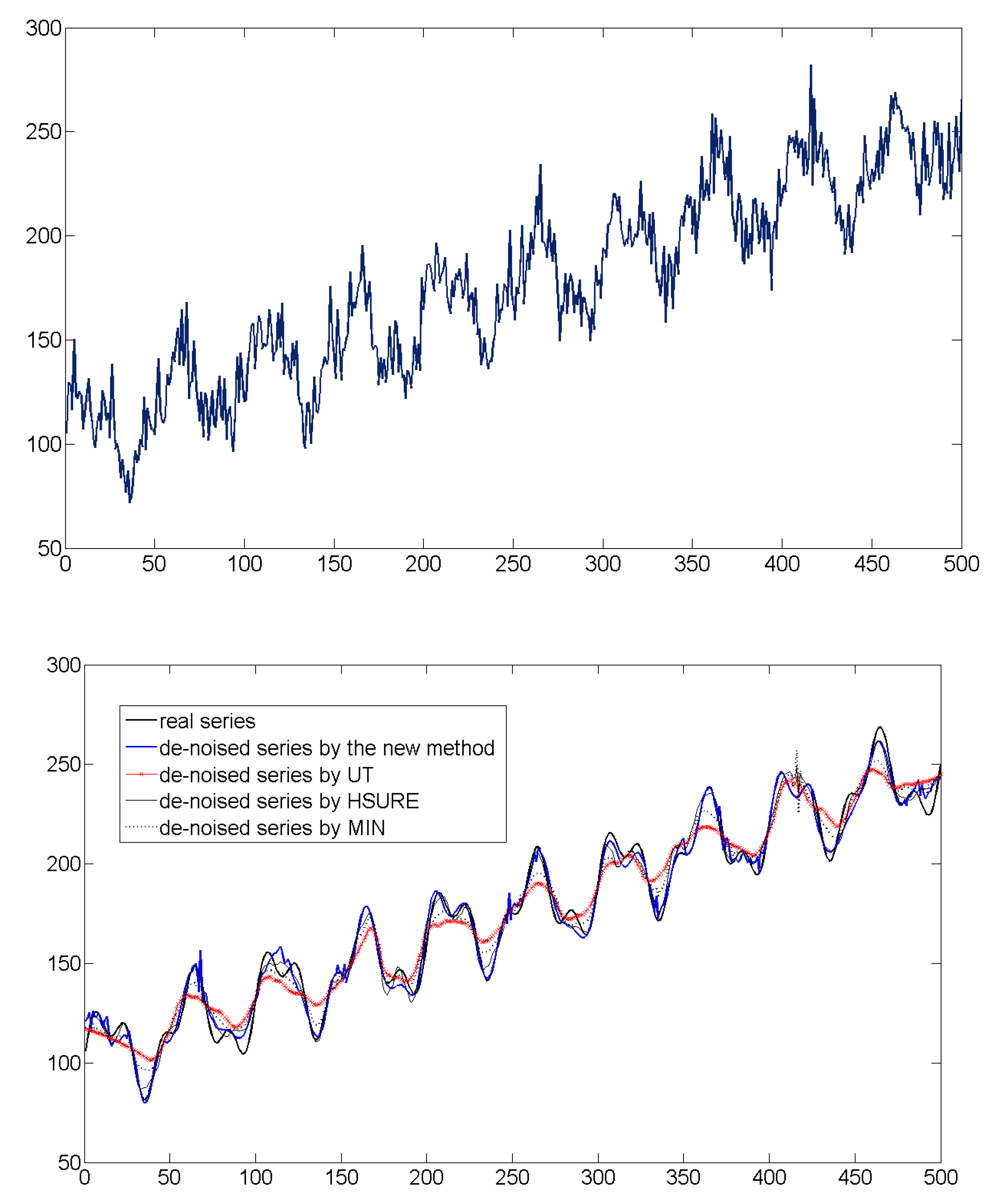
Figure 2.
The synthetic S1 series data (upper) and the de-noising results of S1 series (lower) by using the different methods (in synthetic series S1, noises follow a normal probability distribution).
Figure 2.
The synthetic S1 series data (upper) and the de-noising results of S1 series (lower) by using the different methods (in synthetic series S1, noises follow a normal probability distribution).
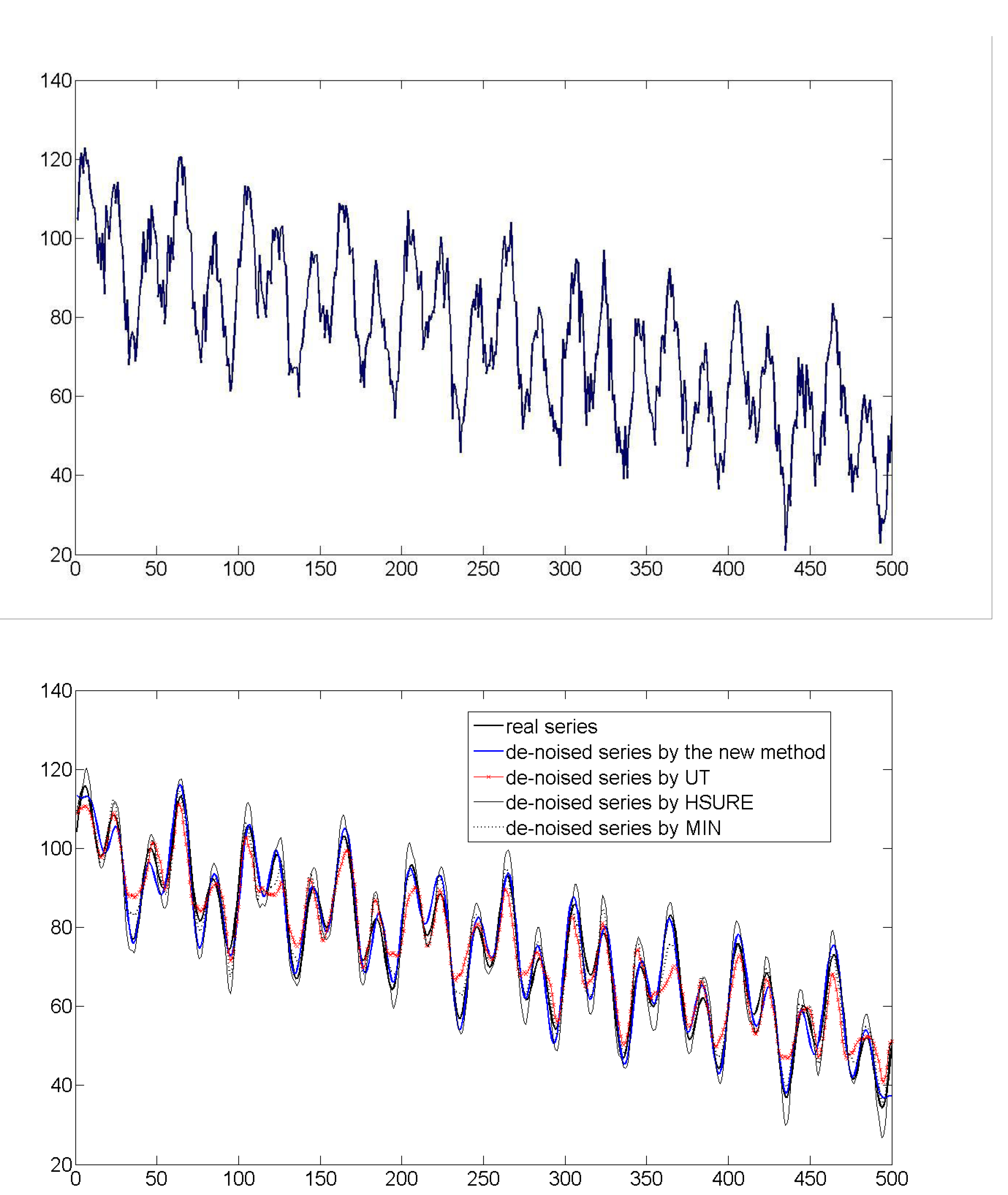
Figure 3.
The synthetic S2 series data (upper) and the de-noising results of S2 series (lower) by using the different methods (In synthetic series S2, noises follow a P-III probability distribution).
Figure 3.
The synthetic S2 series data (upper) and the de-noising results of S2 series (lower) by using the different methods (In synthetic series S2, noises follow a P-III probability distribution).
By comparing and discussing the analysis results of the two synthetic series comprehensively, it can be found that: (1) when using the new method proposed to analyze both the S1 series and the S2 series, the statistical characteristic values of original synthetic series and the main series are very close, and the noises separated show pure random characters. Taking the S1 series for example, the r
1 values of S1 series and the main series are 0.93 and 0.98, respectively; while the r
1 value of the noises separated is 0.08. Besides, the analysis results plotted in
Figure 2 and
Figure 3 also show that the two de-noised series obtained by the new method are very similar to the corresponding real series data, respectively. Thus it is thought that the de-noising results are accurate, and which indicate the reliability of the new method proposed; (2) no matter whether we reduce normal noises in the S1 series or skewed noises in the S2 series, the analysis results of the new entropy-based wavelet de-noising method are in good accord with the criterion proposed in reference [
9]. Therefore, it can hold that the new method proposed not only has its own effectiveness but also has good universality; (3) noises separated from the synthetic series by traditional methods (UT, HSURE and MIN) are different and show good auto-correlations. For examples, r
1 values of noises separated from S1 series are 0.42, –0.26 and 0.26 corresponding to UT, HSURE and MIN, respectively. It means that the analysis results of traditional wavelet de-noising methods are not reasonable and these results should be viewed with caution when used; (4) for the de-noised results of the S1 series and the S2 series by the new method, the values of MSE are 8.21 and 22.35, respectively, which are the lowest in all the analysis results of the methods used. It means that the de-noised series obtained by the new method proposed are the most similar to the real series data, so the analysis results are the most accurate and reliable; (5) by comparing with the analysis results of different de-noising methods, it shows much better performances of the new method proposed in de-noising than other traditional wavelet de-noising methods.
5.2. Observed Time Series Analysis
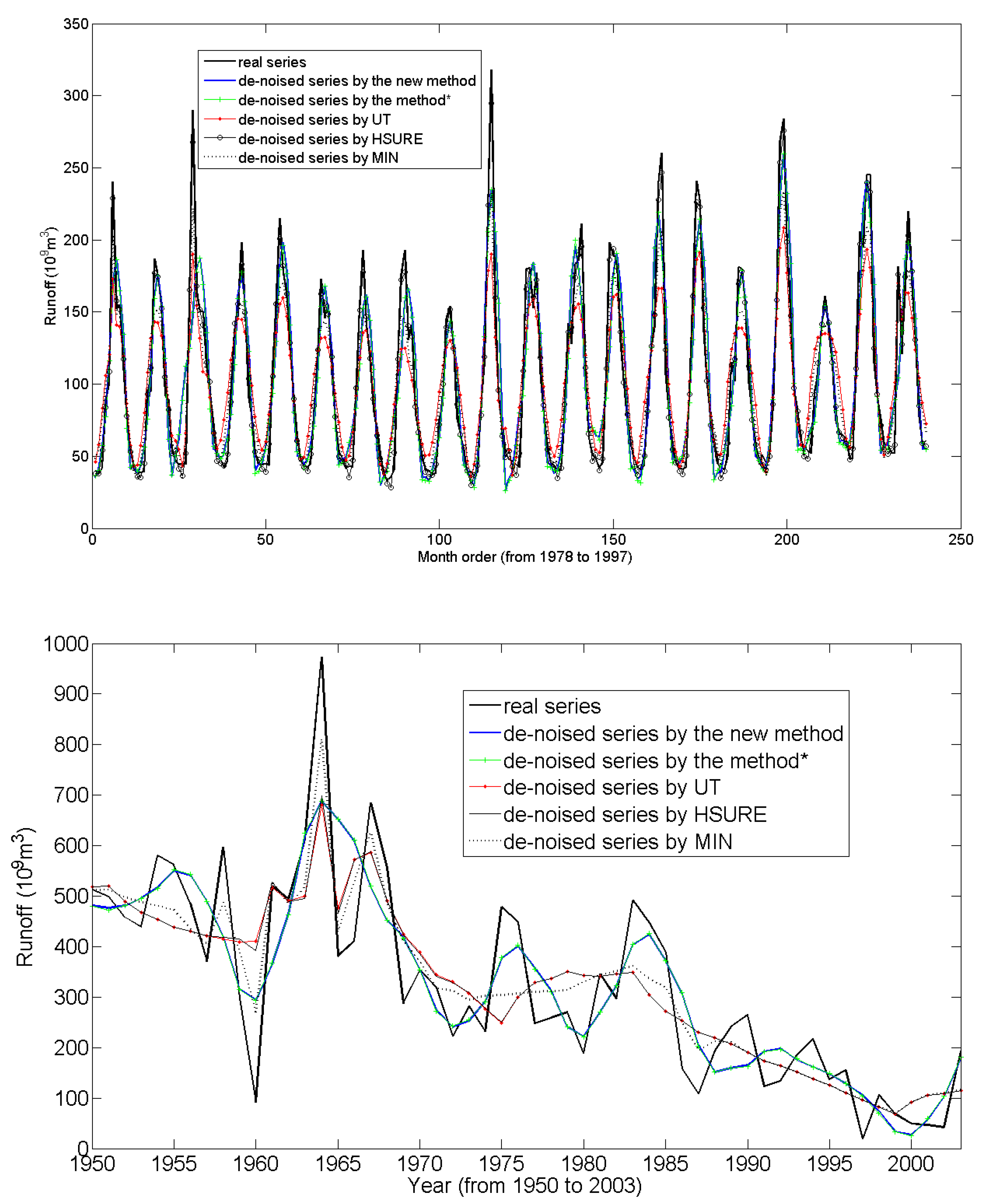
Two hydrologic time series data, RS1 and RS2 for short, are also analyzed by different methods to further verify the performances of the new method proposed. The two hydrologic series data have complex non-stationary and multi-temporal scale characters and are the most representative observed time series data, so in the authors’ opinion, it is deemed that if suitable for analyzing the two hydrologic series data here, the new method proposed can also be used to analyze other observed time series data accurately in practical works.
As illustrated in [
9], RS1 presents 20 years (1978-1997) of monthly runoff series measured at the Dashankou hydrologic station at Kaidu River in Xinjiang province in the northwest of China. There are two recharge sources about Kaidu River, one is snowmelt from Tianshan Mountain, mainly happening from March to April every year, and the other is rainfall, mainly happening at August every year. Consequently two flood seasons happen in every year, and the RS1 series has two obvious periods: about 6 months and 12 months. RS2 presents 54 years (1950-2003) of annual runoff series measured at the Lijin hydrologic station at the estuary area of the Yellow River watershed in the north of China. The Yellow River, the second largest river in China, is an important water source in North China. After the 1970s, because of the great influence of human activities and climatic conditions changes in this area, runoff in the middle and lower Yellow River became seasonal and even presents a cutting-off trend, which causes serious sediment problems and eco-environment problems. Hydrologic regimes in the estuary area are controlled by the whole Yellow River watershed. In present studies, it is shown that the runoff in the Yellow River mainly has four dominant periods: 3, 7, 11 and 18 years.
Analysis of the variation characters (such as periods) of RS1 and RS2 series have great significance in understanding the physical hydrologic processes and for water resources management, as well as many other practical hydrologic works. However, due to the influence of noises, the periods of the two hydrologic series data cannot be identified accurately when analyzing the raw series data directly, especially when analyzing the RS2 series. If the raw series data is de-noised first by a certain method and then periods could be identified accurately, it can be deemed that the de-noising results are reliable and the corresponding de-noising method is effective.
Figure 4.
The de-noising results of RS1 series and RS2 series by different methods (in
Figure 4, “Method*” is the method proposed in reference [
9]).
Figure 4.
The de-noising results of RS1 series and RS2 series by different methods (in
Figure 4, “Method*” is the method proposed in reference [
9]).
According to the analysis results in [
9], here, the P-III probability distribution is used to describe the random characters of noises in the RS1 series, and the normal probability distribution is used to describe the random characters of noises in the RS2 series. Then the two hydrologic series data are analyzed by the new method proposed and three other typical methods (UT, HSURE and MIN). During the analysis process, the “dmey” wavelet is chosen and the maximum time scale level 3 is used to analyze the RS1 series; and the “db2” wavelet is chosen and the maximum time scale level 2 is used to analyze the RS2 series. Finally, the de-noising results of the two observed hydrologic series by different methods are depicted in
Figure 4, and the characteristic values about each of these series data and calculated and summarized in
Table 4 and
Table 5, respectively.
Table 4.
Statistical characteristics of the de-noising results of the RS1 series obtained by different methods.
Table 4.
Statistical characteristics of the de-noising results of the RS1 series obtained by different methods.
| De-noising method | Series types | Statistical characteristic values |
|---|
| σ | r1 | Cs |
|---|
| Original series (RS1) | 101.55 | 61.24 | 0.73 | 0.99 |
| New method proposed | Main series | 101.53 | 57.26 | 0.84 | 0.82 |
| Noises | 0.02 | 14.86 | −0.11 | 0.36 |
| Method* | Main series | 101.53 | 58.32 | 0.82 | 0.77 |
| Noises | 0.02 | 15.07 | −0.16 | 0.33 |
| UT | Main series | 101.74 | 40.97 | 0.84 | 0.35 |
| Noises | −0.19 | 28.08 | 0.42 | 1.15 |
| HSURE | Main series | 101.57 | 59.14 | 0.79 | 0.83 |
| Noises | −0.02 | 7.00 | −0.39 | 0.29 |
| MIN | Main series | 101.76 | 48.24 | 0.82 | 0.57 |
| Noises | −0.29 | 19.42 | 0.29 | 0.96 |
Table 5.
Statistical characteristics of the de-noising results of the RS2 series obtained by different methods.
Table 5.
Statistical characteristics of the de-noising results of the RS2 series obtained by different methods.
| De-noising method | Series types | Statistical characteristic values |
|---|
| σ | r1 | Cs |
|---|
| Original series (RS2) | 324.48 | 194.97 | 0.64 | 0.69 |
| New method proposed | Main series | 323.09 | 164.26 | 0.87 | 0.68 |
| Noises | 1.39 | 65.37 | −0.10 | 0.14 |
| Method* | Main series | 322.81 | 172.39 | 0.86 | 0.70 |
| Noises | 1.67 | 63.31 | −0.13 | 0.11 |
| UT | Main series | 328.75 | 150.43 | 0.91 | 0.32 |
| Noises | −4.27 | 88.34 | 0.34 | 0.30 |
| HSURE | Main series | 325.45 | 179.43 | 0.79 | 0.61 |
| Noises | −0.93 | 44.45 | −0.44 | 0.04 |
| MIN | Main series | 327.57 | 165.06 | 0.81 | 0.60 |
| Noises | −3.09 | 61.28 | −0.21 | 0.08 |
Analysis results in
Table 4 and
Table 5 show that because of the use of Equation (12) to adjust the high frequency wavelet coefficients of DWT, the de-noising results of the new method proposed in the present paper are a little better than those obtained from [
9] and much better than three other traditional methods. Besides, analysis results show that the noises separated from RS1 series follow a skew probability distribution since the value of C
s is bigger than 0.3. Furthermore, the statistical characteristic values of original observed series data, the main series and noises accord well with the criterion proposed in [
9], so it can be deemed that the de-noising results of the two hydrologic time series data are also reasonable and accurate, and the new method proposed is reliable and effective for de-noising. Finally, it can be found that although the real series data in the two observed hydrologic series data are unknown,
Figure 4 shows that compared with the analysis results of other methods, trends of the de-noised series obtained by the new method proposed are more in accordance with the trends of the observed series data as a whole, which means that the new method proposed is comparatively more reliable, and moreover, because noises are reduced accurately and reliably, the periods of the two observed time series data can be identified accurately, as discussed in [
9]. But for the de-noised series of other methods as shown in
Figure 4, they have a little big difference with the de-noised series of the new method, which mean that they also include certain amount of noises or lose some real signals, so all the periods cannot be identified by using them. Since the issue of periods’ identification is far beyond the scope of the present paper, more details about which can be found in detail in reference [
9].
6. Summary and Conclusions
The authenticity and reliability of observed time series data are the very important basis of many applied research and engineering works. In practice, the existence of noises contaminates the real series data and causes many difficulties in time series analysis. When using traditional methods to reduce or remove noises in time series data, the results cannot meet the practical needs. In this paper, in order to overcome the disadvantages of traditional methods and to obtain accurate de-noising results of time series data, by employing information entropy theories to describe the obviously different characters of noises and main series, a new entropy-based wavelet de-noising method has been proposed. By analyzing both synthetic series and typical observed time series data, the performance of the new method proposed has been verified. By comprehensive analysis, the following conclusions about the new method proposed can be drawn: first, because of its basis on information entropy theories to describe the obvious difference of noises and main series in observed series data and then de-noising, the analysis process has a more reliable physical basis and the results of the new method are the global optimum in the whole aspect; secondly, compared with traditional methods, the de-noising results of the new method are more accurate and more reasonable; thirdly, since can be used to analyze both normal noises and skewed noises accurately, the new method shows good effectiveness and universality; and fourthly, the analysis process of the new method is simple and is easy to implement, so it is more applicable and useful in practical applied sciences and engineering works, and therefore, it can be used in future practical applications.
Nevertheless, great attention should be paid to several detailed problems when using the new method, such as determination of the proper probability distribution to describe noises, and choice of a reasonable wavelet function and time scale levels. Only by analyzing and solving these detailed problems accurately, reliable and reasonable de-noising results could be obtained finally.


