Diagnosing a Strong-Fault Model by Conflict and Consistency


Abstract
:1. Introduction
2. Theoretical Background
2.1. Discrete Model
2.1.1. Logic Based Diagnosis Model
- SV (system variable) is the finite set of system variables. The set can be partitioned into mode variables (MODE), observation variables (OBS) and inner variables (INNER). The possible behavioral modes of each component are defined by the mode variable. Observation variables means their values can be obtained from sensors and in this paper (and other most cases) they are assumed to be perfectly correct. And inner variable is all other variables.
- SD (system description) is a finite set of logic propositions which are constraints over SV. Usually SD is represented by CNF or Negative Normal Form (NNF) [28].
- MD (mode distribution) is the prior probability distribution of mode variables.
2.1.2. Weak-Fault Model and Strong-Fault Model
2.2. Diagnosis Problem
- DM is the diagnosis model of a system.
- obs is the assignment set of observation variables.
2.2.1. Diagnosis
2.2.2. Preferred Diagnosis
- P(mode) is the priori probability of mode.
- P(obs|mode) is the conditional probability of observation obs given mode. For simplification, in most cases, P(obs|mode) is restricted in {0, 1} (when there exist conflicts, P(obs|mode) = 0; when there is no conflict, P(obs|mode) = 1) which means the diagnosis is evaluated by priori probability instead of posterior probability. However, the simplification ignores system structure and implies that the existence of conflict is the only flag of if the candidate mode is right, which means that both false alarm and missing alarm are zero. This paper proposes a new scheme to compute it more accurate.
- P(obs) is the marginal probability of observation obs and there is no need to compute it because it is a normalization factor.
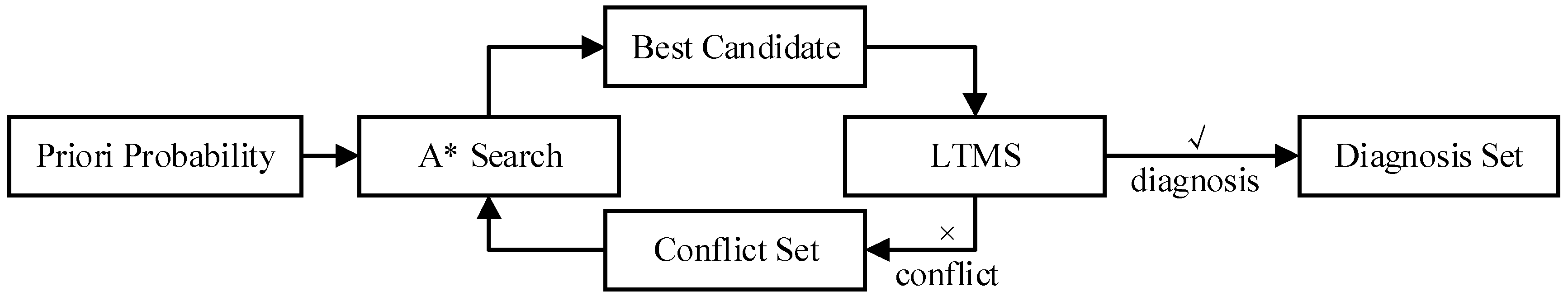
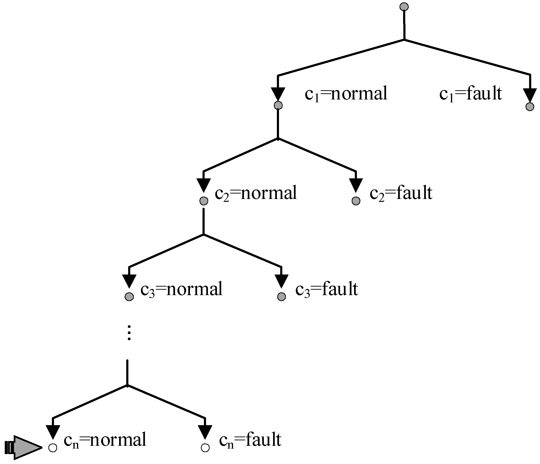
2.3. Conflict Directed A* Search for Weak Model
2.3.1. Single-Diagnosis
2.3.2. Multiple Diagnoses
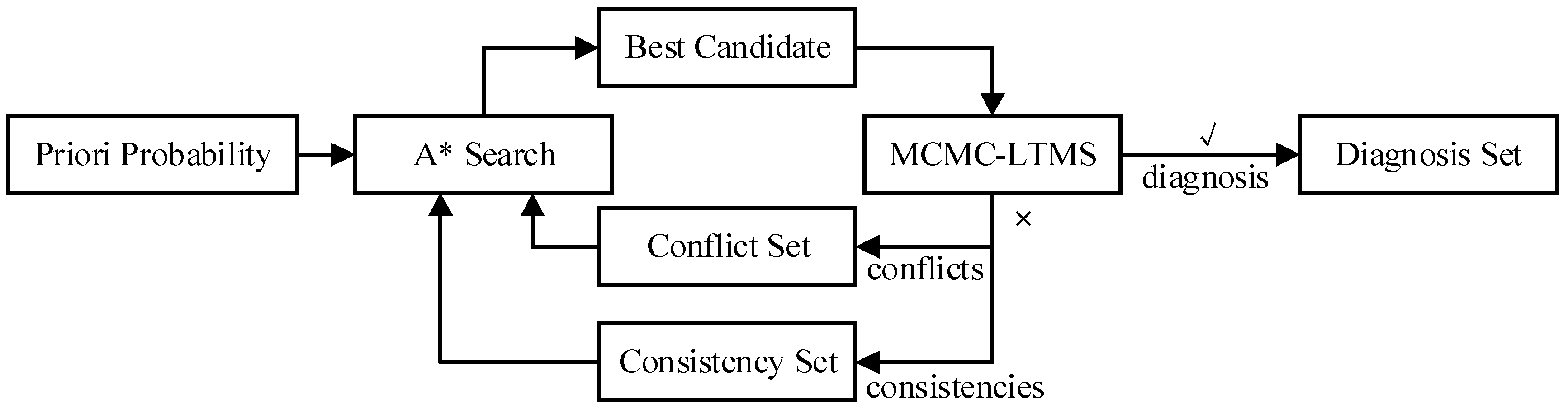
3. Conflict and Consistency Directed A* Diagnosis for a Strong-Fault Model
3.1. Model Encoding
3.2. Multi-Conflict Multi-Consistency LTMS
3.2.1. Multi-Conflict LTMS
3.2.2. Multi-Consistency LTMS
3.2.3. MCMC-LTMS
| Algorithm 1. Pseudocode of CHECK_CONSISTENCY for Multi-Conflict and Multi-Consistency-LTMS (MCMC-LTMS). |
| CHECK_CONSISTENCY (SD, obs, ω) |
| Inputs: SD, system description in the form of CNF obs, observations of observed variables ω, assumptions of mode variables Outputs: the consistency among SD, obs and ω |
| load obs and ω clause_set = SD /* bit0 ~ unit propagate, bit1 ~ conflict or false clause, bit2 ~ true clause */ bit<3> flag0 = 0, flag = 0 do flag = PROPAGATE_FORWARD(clause_set) flag0 = flag0 | flag while (flag ! = 0) conflict = flag0 & (1 << 1) return conflict? false: true |
| Algorithm 2. Pseudocode of PROPAGATE_FORWARD for MCMC-LTMS. |
| PROPAGATE_FORWARD (clause_set) |
| Inputs: clause_set, the clauses describe system Outputs: a 3-bit flag, bit0 ~ unit propagate, bit1 ~ conflict, bit2 ~ true clause clause_set, clause_set is replaced by the clauses remain the same |
| bit<3> flag = 0 for clause in clause_set CLAUSE_SCAN(clause, false_assign, true_assign, unknown_literal)) if(true_assign is not empty) reason = (unknown_literal is empty)? true: false //rule 2 PROPAGATE_TRUE_CLAUSE(clause, true_assign, false_assign, reason)//rule 3 flag = flag | (1<<2) else if(unknown_literal.size > 1) remain_clause.insert(clause) else if(unknown_literal.size == 1) //rule 1 store clause, false_assign, unknown_literal in fringe else PROPAGATE_FALSE_CLAUSE(clause, false_assign) flag = flag | (1<<1) for clause, false_assign, literal in fringe flag = flag | PROPAGATE_FRINGE_CLAUSE(clause, false_assign, literal)?: (1<<0): (1<<1) clause_set = remain_clause return flag |
| Algorithm 3. Pseudocode of MIN_CONFLICTS for MCMC-LTMS. |
| MIN_CONFLICTS (conf_atom_clause) |
| Inputs: conf_atom_clause, a conflict atom, conflict atom set, false clause or false clause set Outputs: the set of minimal conflicts |
| conflict = {} for item in conf_atom_clause if(item is a mode atom and is true) conflict0 = {item} else if(item is a non-mode atom or clause) conflict0 = {} for i in item’s support set conflict0 = MIN_PRODUCT(conflict0, MIN_CONFLICTS(i)) else conflict0 = {} conflict = MIN_PLUS(conflict, conflict0) return conflict |
| Algorithm 4. Pseudocode of MAX_CONSISTENCIES for MCMC-LTMS. |
| MAX_CONSISTENCIESc(atom_true_clause) |
| Inputs: atom_true_clause, an atom, an atom set, a true clause or a true clause set Outputs: the set of maximal consistencies |
| consistency = {} for item in atom_true_clause if(item is a mode atom and is true) consistency0 = {item} else if(item is a non-mode atom or clause) consistency0 = {} for i in item’s support set consistency0 = MAX_PRODUCT(consistency0, MAX_CONSISTENCIES (i)) consistency = MAX_PLUS(consistency, consistency0) return consistency |
3.3. A* Search in Diagnosis
3.3.1. Bayes in Assignments and Possible Conflicts
3.3.2. Single Diagnosis—CCDLSA*
| Algorithm 5. Pseudocode of CCDLSA*. |
| CCDLSA*(SD, obs) |
| Inputs: SD, system description in the form of CNF obs, observations of observed variables Output: ω, the diagnosis consistent with SD and obs |
| ω = all components are normal if(!CHECK_CONSISTENCY(SD, obs, ω)) atom_true_clause = consistency variables or valid true clauses conf_atom_clause = conflict variables or valid false clauses conflicts = {}, fault_components = empty vector consistencies = MAX_CONSISTENCIES(atom_true_clause) do conflicts = conflicts + MIN_CONFLICTS (conf_atom_clause) push back FAULT_COMPONENT(conflicts) - fault_components into fault_components ω = A*_BEST_CANDIDATE(conflicts, consistencies, fault_components) while(!CHECK_CONSISTENCY(SD, obs, ω)) return ω |
| Algorithm 6. Pseudocode of A*_BEST_CANDIDATE for CCDLSA*. |
| A*_BEST_CANDIDATE (conflicts, consistencies, fault_component) |
| Inputs: conflicts, the set of all conflicts consistencies, the set of all consistencies fault_components, the set of possible fault components Output: ω, the best candidate |
| add {} into queue do ω = pop queue if ω does not assign values for all components in fault_components EXPAND(ω, conflicts, consistencies) else break while(1) ω = ADD_DEFAULT(ω) return ω |
3.3.3. Multiple Diagnoses—CCDGA*
| Algorithm 7. Pseudocode of CCDGA*. |
| CCDGA*(SD, obs, k) |
| Inputs: SD, system description in the form of CNF obs, observations of observed variables k, the number of diagnosis want to obtain Output: Ω, the diagnosis set consistent with SD and obs |
| conflicts = {}, consistencies = {} do ω = A*_BEST_CANDIDATE(conflicts, consistencies, all_components) atom_true_clause = consistency variables or valid true clauses in the first consistency check conf_atom_clause = conflict variables or valid false clauses if(!CHECK_CONSISTENCY(SD, obs, ω)) conflicts t = conflicts + MIN_CONFLICTS (conf_atom_clause) consistencies = MAX_CONSISTENCIES(atom_true_clause) in the first consistency check else add ω into Ω while(size of Ω < k) return Ω |
4. Algorithm Analysis
4.1. MCMC-LTMS
4.2. A* Search in Diagnosis
4.2.1. Single Diagnosis—CCDLSA*
4.2.2. Multiple Diagnoses—CCDGA*
5. Case Study
5.1. Model Introduction
5.2. MCMC-LTMS
5.3. A* Search in Diagnosis
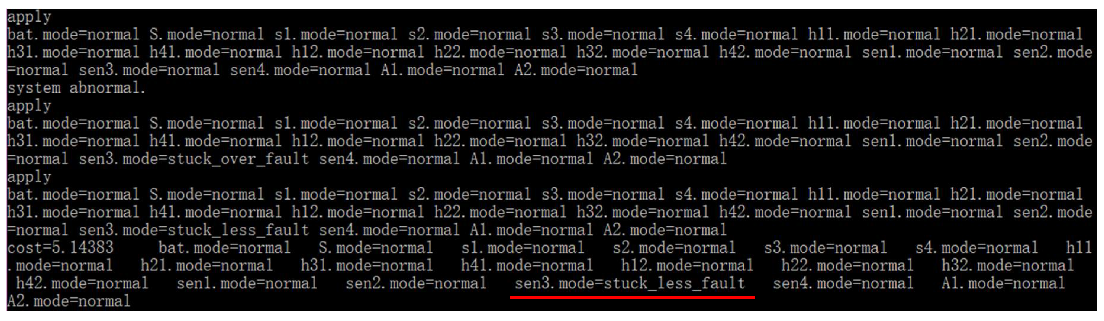
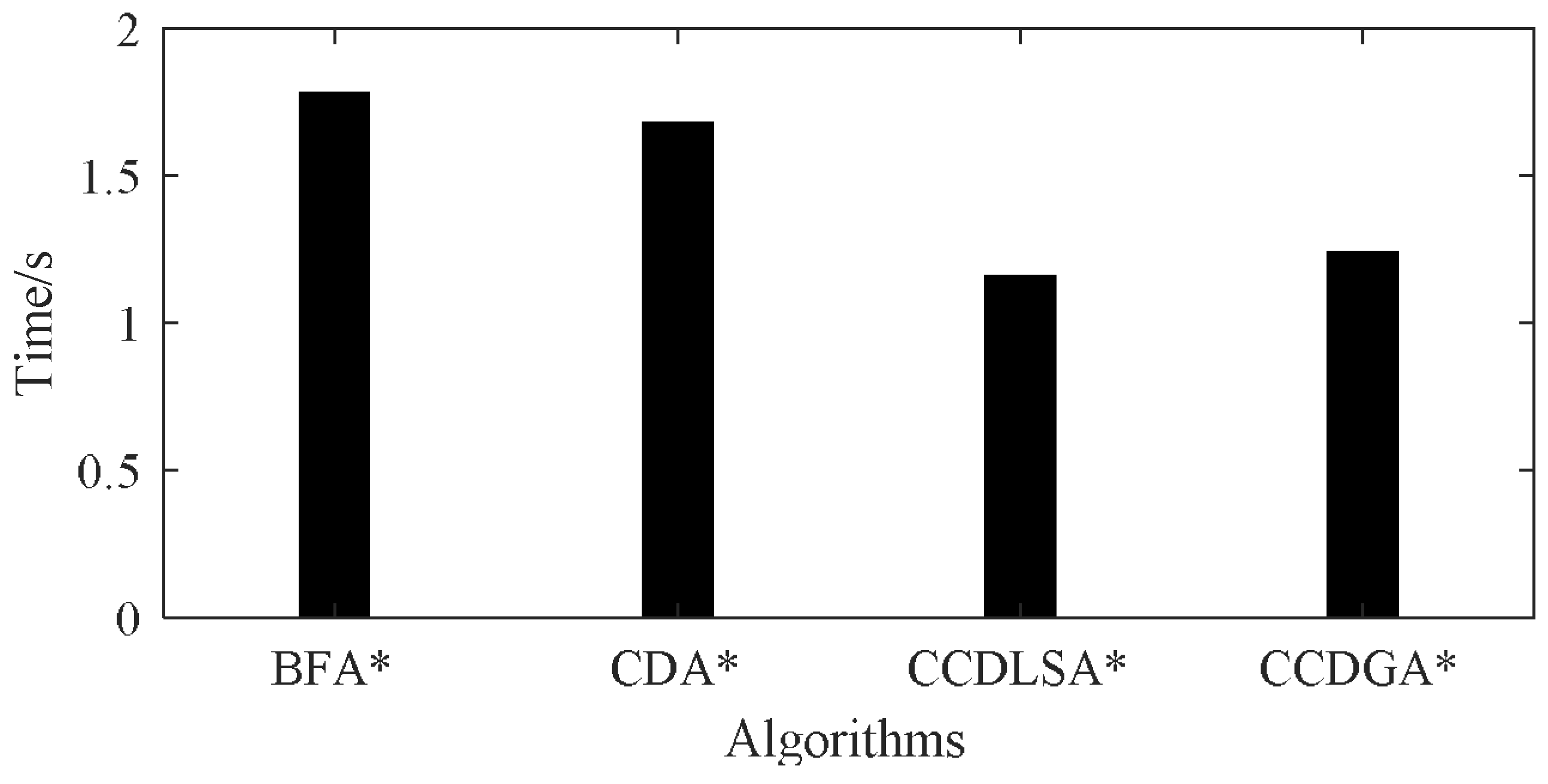
5.3.1. Single Diagnosis
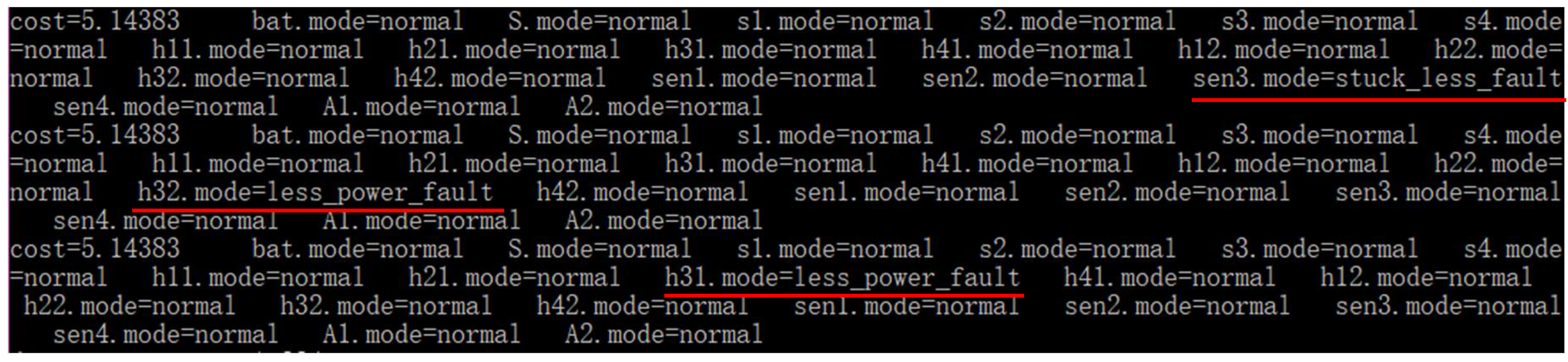
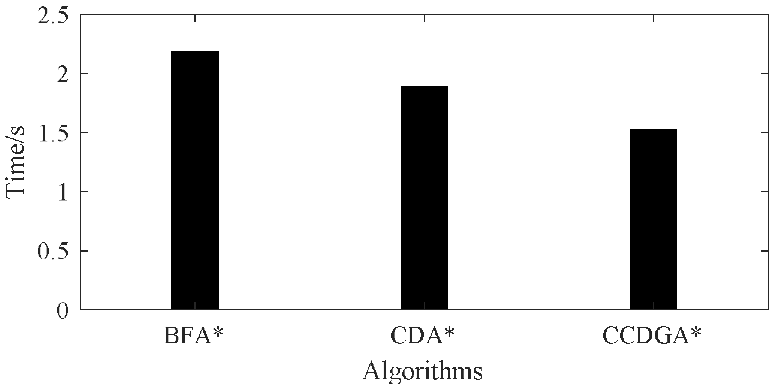
5.3.2. Multiple Diagnoses
6. Conclusions and Future Work
Author Contributions
Conflicts of Interest
References
- Hwang, I.; Kim, S.; Kim, Y.; Seah, C.E. A survey of fault detection, isolation, and reconfiguration methods. IEEE Trans. Control Syst. Technol. 2010, 18, 636–653. [Google Scholar] [CrossRef]
- Nica, I.; Pill, I.; Quaritsch, T.; Wotawa, F. The route to success—A performance comparison of diagnosis algorithms. IJCAI 2013, 13, 1039–1045. [Google Scholar]
- Isermann, R. Fault-Diagnosis Systems: An Introductionfrom Fault Detection to Fault Tolerance; Springer: Berlin, Germany, 2006; ISBN 978-3-540-24112-6. [Google Scholar]
- Gao, Z.; Cecati, C.; Ding, S.X. A Survey of Fault Diagnosis and Fault-Tolerant Techniques Part I: Fault Diagnosis. IEEE Trans. Ind. Electron. 2015, 62, 3757–3767. [Google Scholar] [CrossRef]
- Gao, Z.; Cecati, C.; Ding, S.X. A survey of fault diagnosis and fault-tolerant techniques-part II: Fault diagnosis with knowledge-based and hybrid/active approaches. IEEE Trans. Ind. Electron. 2015, 62, 3768–3774. [Google Scholar] [CrossRef]
- Venkatasubramanian, V.; Rengaswamy, R.; Yin, K.; Kavuri, S.N. A review of process fault detection and diagnosis Part I: Quantitative model-based methods. Comput. Chem. Eng. 2003, 27, 293–311. [Google Scholar] [CrossRef]
- Venkatasubramanian, V.; Rengaswamy, R.; Ka, S.N. A review of process fault detection and diagnosis Part II : Qualitative models and search strategies. Comput. Chem. Eng. 2003, 27, 313–326. [Google Scholar] [CrossRef]
- Venkatasubramanian, V.; Rengaswamy, R.; Kavuri, S.N.; Yin, K. A review of process fault detection and diagnosis part III: Process history based methods. Comput. Chem. Eng. 2003, 27, 327–346. [Google Scholar] [CrossRef]
- Reiter, R. A theory of diagnosis from first principles. Artif. Intell. 1987, 32, 57–95. [Google Scholar] [CrossRef]
- Wang, D.; Yu, M.; Low, C.B.; Arogeti, S. Model-Based Health Monitoring of Hybrid Systems; Springer: New York, NY, USA, 2013; ISBN 978-1-4614-7368-8. [Google Scholar]
- Ding, S.X. Model-Based Fault Diagnosis Techniques; Springer: London, UK, 2013; Volume 53, ISBN 9788578110796. [Google Scholar]
- Qin, S.J. Survey on data-driven industrial process monitoring and diagnosis. Annu. Rev. Control 2012, 36, 220–234. [Google Scholar] [CrossRef]
- Ding, S.X. Data-Driven Design of Fault Diagnosis and Fault-Tolerant Control Systems; Springer: London, UK, 2014; ISBN 978-1-4471-6409-8. [Google Scholar]
- De Kleer, J.; Williams, B.C.; De Kleer, J. Diagnosis with behavioral modes. IJCAI 1989, 89, 1324–1330. [Google Scholar]
- De Kleer, J.; Williams, B.C. Diagnosing multiple faults. Artif. Intell. 1987, 32, 97–130. [Google Scholar] [CrossRef]
- Doyle, J. A Truth Maintenance System. Read. Artif. Intell. 1981, 496–516. [Google Scholar] [CrossRef]
- De Kleer, J. An assumption-based TMS. Artif. Intell. 1986, 28, 127–162. [Google Scholar] [CrossRef]
- Williams, B.C.; Nayak, P.P. A Model-based Approach to Reactive Self-Configuring Systems. In Proceedings of the National Conference on Artificial Intelligence, Portland, OR, USA, 4–8 August 1996; pp. 274–282. [Google Scholar]
- Feldman, A. Approximation Algorithms for Model-Based Diagnosis; TU Delft: Delft, The Netherlands, 2010; ISBN 9789090250236. [Google Scholar]
- Feldman, A.; Provan, G.; Van Gemund, A. Approximate model-based diagnosis using greedy stochastic search. J. Artif. Intell. Res. 2010, 38, 371–413. [Google Scholar] [CrossRef]
- Kurien, J.; Nayak, P. Back to the Future with Consistency-Based Trajectory Tracking. Available online: http://www.aaai.org/Papers/AAAI/2000/AAAI00-057.pdf (accessed on 27 March 2018).
- Williams, B.C.; Ragno, R.J. Conflict-Directed A* and Its Role in Model-Based Embedded Systems. Discret. Appl. Math. 2007, 155, 1562–1595. [Google Scholar] [CrossRef]
- Forbus, K.D.; de Kleer, J. Building Problem Solvers (Artificial Intelligence); The MIT Press: London, UK, 1993; ISBN 0262061570. [Google Scholar]
- Stern, R.; Kalech, M.; Feldman, A.; Provan, G. Exploring the Duality in Conflict-Directed Model-Based Diagnosis. In Proceedings of the Twenty-Sixth AAAI Conference on Artificial Intelligence, Toronto, ON, Canada, 22–26 July 2012; pp. 828–834. [Google Scholar]
- Shchekotykhin, K.; Jannach, D.; Schmitz, T. MERGEXPLAIN: Fast computation of multiple conflicts for diagnosis. IJCAI 2015, 15, 3221–3228. [Google Scholar]
- Shchekotykhin, K.; Jannach, D.; Schmitz, T. A divide-and-conquer-method for computing multiple conflicts for diagnosis. CEUR Workshop Proc. 2015, 1507, 3–10. [Google Scholar]
- Junker, U. QuickXplain: Preferred Explanations and Relaxations for Over-Constrained Problems. In Proceedings of the Nineteenth AAAI Conference on Artificial Intelligence, San Jose, CA, USA, 25–29 July 2004; pp. 167–172. [Google Scholar]
- Darwiche, A. Decomposable Negation Normal Form. J. ACM 2001, 48, 608–647. [Google Scholar] [CrossRef]
- Torta, G. Compact Representation of Diagnoses for Improving Efficiency in Model Based Diagnosis. Ph.D. Thesis, Universita di Torino, Torino, Italy, 2006. [Google Scholar]
- Biere, A.H.; Heule, M.; van Maaren, H.; Walsh, T. Handbook of Satisfability; IOS: Amsterdam, The Netherlands, 2009; ISBN 978-1-58603-929-5. [Google Scholar]
- Dechter, R. Constraint Processing; Morgan Kaufmann: Burlington, MA, USA, 2003; Volume 33, ISBN 978-1-55-860890-0. [Google Scholar]
- Pulido, B.; González, C.A. Possible conflicts: A compilation technique for consistency-based diagnosis. IEEE Trans. Syst. Man Cybern. Part B Cybern. 2004, 34, 2192–2206. [Google Scholar] [CrossRef]
- Russell, S.; Norvig, P. Artificial Intelligence a Modern Approach; Pearson Education: Upper Saddle River, NJ, USA, 2013; ISBN 9780136042594. [Google Scholar]


| Mode Assignments | PCj | Conditional Probability |
|---|---|---|
| f is the number of wrong assignments | 1 | εf |
| 0 | 1 − εf |
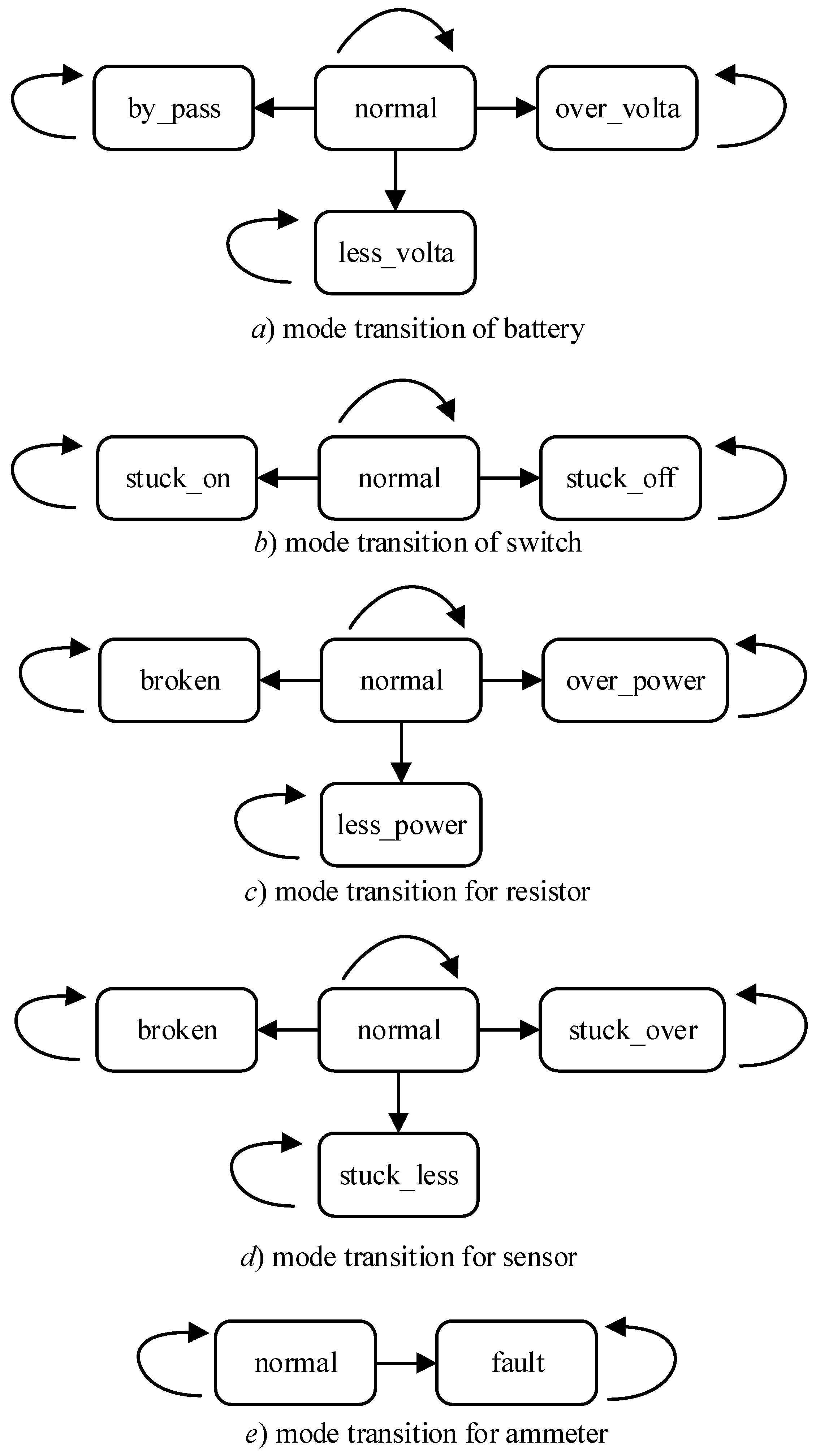
| Component | Mode | Behavior |
|---|---|---|
| battery | normal | The output voltage is normal. |
| by_pass | The output voltage is zero. | |
| less_volta | The output voltage is lower than normal. | |
| over_volta | The output voltage is higher than normal. | |
| switch | normal | When the switch is on, output is equal to the input. Zero when off. |
| stuck_on | The switch keeps on ignoring the command. | |
| stuck_off | The switch keeps off ignoring the command. | |
| resistor | normal | If the input voltage is zero, there is no heat and output current is zero. If the input voltage is less, power is less and output current exists. If the input voltage is normal, power is normal and output current exists. If the input voltage is over, power is over and output current exists. |
| less_power | If the input voltage is zero, there is no heat and output current is zero. Otherwise, power is less and output current exists. | |
| over_power | If the input voltage is zero, no heat and output current is zero. Otherwise, power is less and output current exists. | |
| broken | There is no heat and output current is zero. | |
| sensor | normal | If both resistors generate no heat, output temperature is none. If both resistors generate heat normally or one is less power but the other is over power, output temperature is normal. If one resistor generates heat over power and the other one is normal or over power, output temperature is over. In other cases, output temperature is less. |
| stuck_less | Output temperature is less. | |
| stuck_over | Output temperature is over. | |
| broken | Output temperature is broken. | |
| ammeter | normal | The output is the number of input currents. |
| fault | The output is always zero. |
| Variable | cS | cs1 | cs2 | cs3 | cs4 | t1 | t2 | t3 | t4 | c1 | c2 |
|---|---|---|---|---|---|---|---|---|---|---|---|
| Value | true | true | true | true | true | norm | norm | less | norm | four | four |
| Type | Set |
|---|---|
| Conflict | {battery, S, s3, h31, h32, sen3} |
| Consistency | {battery, S, s1, h11, h12, sen1} |
| {battery, S, s2, h21, h22, sen2} | |
| {battery, S, s4, h41, h42, sen4} | |
| {battery, S, s1, s2, h11, h12, h21, h22, A1} | |
| {battery, S, s3, s4, h31, h32, h41, h42, A2} |
| Algorithm | 1 | 2 | 3 | 4 | 5 | 6 | 7 | 8 | 9 | 10 | Ave | Ratio |
|---|---|---|---|---|---|---|---|---|---|---|---|---|
| BFA* | 1.787 | 1.711 | 1.620 | 1.712 | 1.738 | 1.883 | 1.702 | 1.782 | 1.738 | 1.680 | 1.74 | 100.00% |
| CDA* | 1.644 | 1.756 | 1.711 | 1.668 | 1.676 | 1.640 | 1.687 | 1.650 | 1.682 | 1.64 | 1.68 | 96.55% |
| CCDLSA* | 1.165 | 1.163 | 1.156 | 1.169 | 1.131 | 1.19 | 1.134 | 1.144 | 1.147 | 1.153 | 1.16 | 66.67% |
| CCDGA* | 1.191 | 1.24 | 1.252 | 1.311 | 1.183 | 1.183 | 1.178 | 1.256 | 1.267 | 1.319 | 1.24 | 71.26% |
| Algorithm | BFA* | CDA* | CCDLSA* | CCDGA* | ||||
|---|---|---|---|---|---|---|---|---|
| Num | Ratio | Num | Ratio | Num | Ratio | Num | Ratio | |
| Tried Candidates | 11 | 100.00% | 8 | 72.72% | 3 | 27.27% | 3 | 27.27% |
| Expanded Nodes | 125 | 100.00% | 116 | 92.80% | 6 | 4.80% | 23 | 18.40% |
| Nodes in Queue | 293 | 100.00% | 286 | 97.61% | 15 | 5.12% | 55 | 18.77% |
| Algorithm | 1 | 2 | 3 | 4 | 5 | 6 | 7 | 8 | 9 | 10 | Ave | Ratio |
|---|---|---|---|---|---|---|---|---|---|---|---|---|
| BFA* | 2.326 | 2.234 | 2.228 | 2.179 | 2.146 | 2.152 | 2.060 | 2.227 | 2.122 | 2.163 | 2.18 | 100.00% |
| CDA* | 1.844 | 1.951 | 2.053 | 1.823 | 1.881 | 1.871 | 1.815 | 1.871 | 1.890 | 1.892 | 1.89 | 86.70% |
| CCDGA* | 1.347 | 1.593 | 1.465 | 1.642 | 1.534 | 1.517 | 1.477 | 1.496 | 1.482 | 1.524 | 1.52 | 69.72% |
| Algorithm | BFA* | CDA* | CCDGA* | |||
|---|---|---|---|---|---|---|
| Num | Ratio | Num | Ratio | Num | Ratio | |
| Tried Candidates | 35 | 100.00% | 14 | 40.00% | 9 | 25.71% |
| Expanded Nodes | 297 | 100.00% | 234 | 78.79% | 78 | 26.26% |
| Nodes in Queue | 689 | 100.00% | 610 | 88.53% | 190 | 27.58% |
© 2018 by the authors. Licensee MDPI, Basel, Switzerland. This article is an open access article distributed under the terms and conditions of the Creative Commons Attribution (CC BY) license (http://creativecommons.org/licenses/by/4.0/).
Share and Cite
Zhang, W.; Zhao, Q.; Zhao, H.; Zhou, G.; Feng, W. Diagnosing a Strong-Fault Model by Conflict and Consistency. Sensors 2018, 18, 1016. https://doi.org/10.3390/s18041016
Zhang W, Zhao Q, Zhao H, Zhou G, Feng W. Diagnosing a Strong-Fault Model by Conflict and Consistency. Sensors. 2018; 18(4):1016. https://doi.org/10.3390/s18041016
Chicago/Turabian StyleZhang, Wenfeng, Qi Zhao, Hongbo Zhao, Gan Zhou, and Wenquan Feng. 2018. "Diagnosing a Strong-Fault Model by Conflict and Consistency" Sensors 18, no. 4: 1016. https://doi.org/10.3390/s18041016
APA StyleZhang, W., Zhao, Q., Zhao, H., Zhou, G., & Feng, W. (2018). Diagnosing a Strong-Fault Model by Conflict and Consistency. Sensors, 18(4), 1016. https://doi.org/10.3390/s18041016